One-dimensional turbulence: model formulation and ...

J. Fluid Mech. (1999), vol. 392, pp. 277–334. c 1999 Cambridge University Press

277

Printed in the United Kingdom

One-dimensional turbulence: model formulation and application to homogeneous turbulence, shear flows, and buoyant stratified flows By A L A N R. K E R S T E I N Combustion Research Facility, Sandia National Laboratories, Livermore, CA 94551-0969, USA (Received 18 February 1997 and in revised form 1 March 1999)

A stochastic model, implemented as a Monte Carlo simulation, is used to compute statistical properties of velocity and scalar fields in stationary and decaying homogeneous turbulence, shear flow, and various buoyant stratified flows. Turbulent advection is represented by a random sequence of maps applied to a one-dimensional computational domain. Profiles of advected scalars and of one velocity component evolve on this domain. The rate expression governing the mapping sequence reflects turbulence production mechanisms. Viscous effects are implemented concurrently. Various flows of interest are simulated by applying appropriate initial and boundary conditions to the velocity profile. Simulated flow microstructure reproduces the − 53 power-law scaling of the inertial-range energy spectrum and the dissipationrange spectral collapse based on the Kolmogorov microscale. Diverse behaviours of constant-density shear flows and buoyant stratified flows are reproduced, in some instances suggesting new interpretations of observed phenomena. Collectively, the results demonstrate that a variety of turbulent flow phenomena can be captured in a concise representation of the interplay of advection, molecular transport, and buoyant forcing.

Contents 1. Introduction 2. Model formulation 2.1. Overview 2.2. Advection 2.3. Viscosity 2.4. Buoyancy 2.5. Parameter evaluation 3. Homogeneous turbulence 3.1. Eddy cascade 3.2. Numerical results 4. Wall-bounded flow 5. Buoyancy-driven flow 5.1. Homogeneous buoyancy-driven turbulence 5.2. Rayleigh convection 5.3. Penetrative convection

278 279 279 280 284 286 289 290 290 293 299 302 302 304 311

278 A. R. Kerstein 6. Stratified boundary layers 6.1. Monin–Obukhov similarity 6.2. Implications for atmospheric-boundary-layer modelling 6.3. Shear-driven entrainment 7. Discussion Appendix A Appendix B Appendix C

315 315 318 318 322 324 327 329

1. Introduction One-dimensional models of turbulent flows have been introduced in various contexts. Eddy-diffusivity formulations are often used to model ensemble-averaged flow structure in one direction, typically the vertical direction in buoyant stratified flows. One-dimensional representations of the evolution of individual flow realizations have also been formulated, such as the randomly forced Burgers equation (Chekhlov & Yakhot 1995), a one-dimensional Biot-Savart formulation (Constantin, Lax & Majda 1985; De Gregorio 1990), and one-dimensional binary-tree formulations (Aurell, Dormy & Frick 1997; Benzi et al. 1997). Here, a one-dimensional simulation of individual flow realizations, denoted ‘onedimensional turbulence’ (ODT), is formulated whose distinctive feature is the representation of turbulent advection by a postulated stochastic process rather than an evolution equation. Viscosity is incorporated as a concurrent deterministic process, governed by an evolution equation of conventional form. In ODT, turbulent advection is represented by a random sequence of eddy motions. Each eddy motion is an instantaneous mapping of a segment of the one-dimensional domain onto itself. The eddy size (i.e. the size of the affected segment) and the time and location of its occurrence are chosen according to a random process reflecting kinetic-energy production mechanisms. The one-dimensional domain represents a transverse direction in planar coordinates. (Implementation in cylindrical coordinates is feasible, but is not considered here.) For turbulent flows that develop temporally, flow evolution is represented by the time evolution of a streamwise velocity profile on the one-dimensional domain. For spatially developing flows, simulated flow evolution represents streamwise spatial development. The streamwise velocity profile has two roles: it represents the strain field that generates eddy motions, and it is the observable whose statistics are compared to experimental results. Kinematical aspects of advection are represented in two dimensions, though the computational domain is one-dimensional. The eddies induce motion along the one-dimensional coordinate, while the observable corresponds to streamwise flow, perpendicular to the one-dimensional coordinate. Thus, the Reynolds stress profile hu0 v 0 i can be obtained, despite the lack of an explicit v profile, by monitoring the transverse flux of u induced by eddy motions. The model incorporates viscosity as well as advection. Viscous evolution is implemented by solving the appropriate transport equation for the velocity field on the one-dimensional domain. This evolution is nominally a continuous-time process, though time discretization is required for numerical implementation. This continuous evolution is punctuated by the instantaneous mapping events representing eddies. The concurrent viscous and advective processes are interactive because each process modifies the velocity field that governs both processes. Computationally affordable

One-dimensional turbulence

279

resolution of viscous scales in fully developed turbulence is a key attribute of the one-dimensional formulation. Resolution of molecular transport scales allows inclusion of diffusive scalars with no additional approximations, facilitating application of the model to turbulent dispersion, heat transfer, chemically reacting flows, etc. Scalar mixing processes that are sensitive to fine-scale turbulent motions motivated the author’s earlier development (Kerstein 1991) of the linear-eddy model (LEM). That model likewise involves fully resolved molecular transport of scalars on a one-dimensional domain, concurrent with a random sequence of events representing turbulent eddies. In the LEM, flow properties are specified empirically by assigning parameters governing the random event sequence. There is no provision for feedback of local flow properties to the random process governing subsequent events. In contrast, ODT is formulated so as to capture this feedback with minimal empiricism. In this regard, ODT is both a turbulence model and a methodology for fully resolved simulation of mixing, chemical reaction, and related scalar processes in turbulence. The latter capability is a key feature distinguishing ODT from conventional turbulence models that require the incorporation of mixing submodels in order to treat scalar processes. Because ODT subsumes many of the previously demonstrated capabilities of the LEM with regard to mixing, the emphasis here is on flow properties. It is noted that comparable or superior predictions of particular flow properties may be obtained using conventional models. The distinguishing features of ODT are its scope, simplicity, minimal empiricism, and capability to incorporate complex molecular processes (variable transport properties, chemical reactions, dynamically active scalars, etc.) without introducing additional approximations. Because ODT is a fully resolved simulation, various statistical quantities can be extracted that are not provided by conventional closure methods, such as single-point and multipoint moments of any order, multivariate probability density functions, conditional statistics, power spectra, level-crossing statistics, Lagrangian statistics, and fractal dimensions. Only a limited exploration of these possibilities is attempted here. A one-dimensional formulation is applicable only to flows that are homogeneous in at least one spatial coordinate. Many flows of fundamental interest and practical importance are of this type. For more complex flows, a one-dimensional unsteady simulation may prove advantageous as a subgrid model within a large-eddy simulation or a multidimensional steady-state model. Implementation of the LEM in this manner has been demonstrated (Menon & Calhoon 1996). The model is formulated in § 2. Additional details, including numerical implementation issues, are discussed in Appendix A. Relationships between model quantities and three-dimensional flow properties are examined in Appendices B and C. The remainder of the paper addresses various applications, which indicate the diversity of flow configurations and phenomena that can be treated. Many of the computed behaviours are direct consequences of the formulation, but in several instances new insights are gained concerning phenomena that are not yet well understood.

2. Model formulation 2.1. Overview Operationally, ODT is a numerical method for generating realizations of a class of stochastic initial-boundary-value problems on a one-dimensional domain. For

280

A. R. Kerstein

temporal flows (T-flows), each ODT realization represents a time history, u(y, t), of the transverse profile of streamwise velocity, and/or time histories of one or more scalar profiles, generically denoted θ(y, t). For spatially developing flows (S-flows), ODT generates realizations parameterized by (y, x) instead of (y, t), where x is the streamwise coordinate. (Here, the y-coordinate is normal to the streamwise and spanwise directions.) It is convenient to describe ODT with reference to T-flow, later explaining distinct features of the S-flow formulation. Eddy motions are governed by the strain field as characterized by variations of the instantaneous streamwise velocity u(y, t) along the y-coordinate, and by analogous variations of the instantaneous buoyancy profile. For three-dimensional continuum flow, the link between these turbulence production mechanisms and the induced motions is the Navier–Stokes equation, which governs viscous as well as advective flow evolution. In ODT, the production mechanisms, the induced motions, and viscous transport are distinct entities. The time evolution of u(y, t) is governed by viscous transport, whose continuum evolution is analogous to Navier–Stokes viscous transport, and a concurrent advection process consisting of a stochastic sequence of mappings applied to the one-dimensional domain. Likewise, each scalar profile is subject to molecular-diffusive transport based on the appropriate diffusion coefficient, and the same mapping sequence that is applied to u(y, t). The mapping rule and the rate expression that govern the stochastic event sequence are discussed in § 2.2, and viscous evolution is discussed in § 2.3. 2.2. Advection 2.2.1. The one-dimensional eddy In ODT, each eddy is an instantaneous event. Having no time duration, it has no opportunity to interact directly with other eddies. Rather, the interaction is indirect, mediated by the velocity profile u(y, t) and/or profiles of dynamically active scalars such as the density ρ(y, t) in buoyant stratified flow. For clarity, consideration of variable-density flow is deferred until § 2.4. An individual event is a mapping that determines a new streamwise velocity profile ˆ u(y) as a function of a given profile u(y). (Here and subsequently, the argument t is suppressed where the meaning is clear.) The velocity profile is deemed to be unaffected outside a selected interval y0 6 y 6 y0 + l, where l represents the eddy size. Thus, ˆ u(y) = u(y) for y outside [y0 , y0 + l]. To specify the functional dependence in [y0 , y0 +l], it is useful to adopt a Lagrangian viewpoint with respect to the y-coordinate. In this context, the effect of an eddy on u(y) involves two mechanisms: transverse displacement of fluid elements and modification of the streamwise velocity within fluid elements. Taking the one-dimensional domain to be a closed system, incompressibility constrains the transverse displacements associated with the eddy to be a measurepreserving map of the domain onto itself. Namely, the displacements can be repreR R ˆ sented by a mapping y(y) such that Sˆ dyˆ = S dy, where S is any subset of the y ˆ domain and Sˆ is the image of S on y. ˆ to be a continuous function of y. ˆ This It is desirable for the inverse mapping y(y) property ensures that two fluid elements that are close to each other after the mapping were close to each other prior to the mapping, thus preventing the introduction of discontinuities into the velocity profile. ˆ the map y(y) is required to be measure-preserving, all velocity moments R Because un (y) dy are preserved by the map. (This property is analogous to the constancy of


281

area-integrated vorticity moments in incompressible two-dimensional Euler flow.) In particular, the total streamwise momentum (n = 1) and energy (n = 2) are preserved. (For S-flow, u and u2 are volume flux and momentum flux, respectively.) Streamwise momentum and energy conservation (volume-flux and momentum-flux conservation for S-flow) are essential properties, but the higher streamwise invariants are artifacts. An additional artifact is that energy conservation is here enforced on a particular velocity component. These constraints do not arise in three-dimensional flow owing to the second eddy mechanism: modification of the streamwise velocity within fluid elements. Namely, the pressure-gradient term of the Navier–Stokes equation modifies velocity components and thus the orientation of the velocity vector, inducing energy redistribution among velocity components. Here, this mechanism is omitted. This simplification necessarily fails for flows in which imposed pressure gradients drastically alter the flow structure, such as separating boundary layers. Even in the absence of imposed pressure gradients, pressure fluctuations can have important effects whose omission may have an impact on the performance of the model. ˆ The ODT representation of an eddy is thus a mapping rule y(y) that reflects only one of two mechanisms of u(y) modification by an eddy. Moreover, the mechanism that is represented is purely kinematical. However, aspects of turbulence energetics are incorporated into the rule that determines the stochastic sequence of mapping events (§ 2.4.1). An important consequence of the proposed eddy representation is that the effect of an eddy on u(y) is the same as on a passively advected scalar profile. If P r = 1 and the scalar and streamwise velocity have the same initial and boundary conditions, then the scalar and velocity profiles evolve identically. In effect, the Reynolds analogy is exact in ODT for P r = 1. This implies P rT = 1, where P rT is the turbulent Prandtl number. Measured values of P rT typically differ from unity by about 10 or 20%, lending some preliminary support to the kinematical approach. Monin & Yaglom (1971) note that mixing-length theories likewise formulate the transfer of momentum as the transfer of a passive scalar, neglecting pressure-induced momentum changes within fluid elements. This consideration led Taylor (1932) to formulate a vorticity transfer theory based on the proposition that vorticity is transported more nearly as a passive scalar than is momentum. This proposition is based on the exact analogy between vorticity and passive-scalar transport in two-dimensional inviscid flow. In three dimensions, the analogy is less justified, so a vorticity formulation is not necessarily advantageous (Monin & Yaglom 1971). A velocity rather than a vorticity formulation is adopted in ODT, owing to its simplicity and ease of interpretation. ˆ The mapping rule y(y) that is adopted is the ‘triplet map’ employed in the LEM (Kerstein 1991). The rule is stated here in a more general form, although only the particular form defined previously is implemented. In [y0 , y0 + l], yˆ is taken to be a three-valued function of y, as follows: ( y0 + f1 (y − y0 ) (2.1) yˆ = y0 + f2 l − (f2 − f1 )(y − y0 ) y0 + f2 l + (1 − f2 )(y − y0 ). Equation (2.1) maps the interval [y0 , y0 +l] onto each of three subintervals [y0 , y0 +f1 l], [y0 + f1 l, y0 + f2 l] and [y0 + f2 l, y0 + l], where 0 < f1 < f2 < 1. As in LEM applications, the choice f1 = 13 , f2 = 23 is implemented in all cases.

282

A. R. Kerstein (a)

(c)

(b)

Figure 1. Effect of the triplet map on an initially linear velocity profile u(y, t). (a) Initial profile. (b) Velocity profile after applying the triplet map to the interval denoted by ticks. (c) Discrete representation of the initial profile, and illustration of the effect of a triplet map on an interval consisting of nine cells. For clarity, arrows indicating formation of the central of the three images of the original interval are dashed.

For this choice, figure 1 illustrates the effect on a linear profile u(y) ∼ y. The effect is to replace the profile in [y0 , y0 + l] by three compressed images of the original, with the middle image inverted (flipped). This map reflects the compressive and rotational attributes of eddy motion, as discussed in detail previously (Kerstein 1991). It causes multiplicative increase of strain intensity and a corresponding multiplicative decrease of strain length-scale. As discussed in § 3.1, these features lead to a self-similar eddy cascade. The choice f1 = 13 , f2 = 23 is simplest because it gives uniform strain intensity multiplication and length-scale reduction within the eddy. Other choices would introduce spatial variation of these properties within the eddy, governed by two empirical parameters (or one if the symmetry f1 = 1 − f2 is imposed). Allowing this empiricism might be beneficial in some contexts. For example, f1 = 1 − f2 1 would represent a mildly compressive rotation in between thin high-compression zones. This might increase the intermittency of the eddy cascade, and in the context of buoyant stratified flow, might represent convective structures that overturn with little length-scale reduction except in the high-strain regions on their periphery. Although (2.1) is nominally a three-valued mapping, it can be approximated on a discretized computational domain by a single-valued mapping that is simply a permutation of the cells within the mapping interval [y0 , y0 + l], and thus is measurepreserving. The permutation rule, stated in its general form in Kerstein (1991), is illustrated for a particular case in figure 1(c). That figure illustrates the continuity of the inverse mapping, as follows. Fluid elements that are nearest neighbours in the transformed profile are no more than


283

three cells apart in the preimage. In contrast, nearest neighbours in the preimage can be separated by more than half the eddy size in the transformed profile. This distinction is minor for the nine-cell discretization illustrated in the figure, but becomes increasingly significant as spatial resolution is improved. By considering the limit of vanishing cell size, it can be shown formally that the inverse mapping is continuous but that the forward mapping is discontinuous almost everywhere within the mapping interval [y0 , y0 + l]. 2.2.2. Eddy rate distribution As in the LEM, mapping events are governed by an ‘eddy rate distribution’ λ(l), where λ(l) dl is the frequency of events in the size range [l, l + dl] per unit length along the y-coordinate. Based on this definition, λ(l) has units (length2 × time)−1 . The dimensional relation (2.2) λ(l) = 1/[l 2 τ(l)] expresses λ(l) in terms of a time τ(l) that is interpreted as an eddy time scale. A free parameter, to be determined empirically, could be inserted in (2.2). This is not done here because the principal objective here is to address qualitative behaviours with minimal empiricism. For reasons explained shortly, a free parameter is included in the expression for τ. In the LEM, τ(l) is taken to be a mean time scale estimated by invoking the usual turbulence phenomenology. Here, this picture is modified by treating τ(l) as a local, instantaneous time scale, now denoted τ(l; y, t), whose evaluation is based on u(y, t). Dimensional reasoning suggests that τ(l; y, t) is determined by the local strain du(y, t)/dy, as discussed in § 2.1. A refinement of this proposal that accounts for the finite spatial extent of an eddy is motivated by a Fourier picture corresponding to the parameterization k = 1/l. Viewing individual eddies as Fourier wave packets (Tennekes 1976), the eddy time scale can be expressed in the form τk (y, t) ∼ 1/[kuk (y, t)]. Here, kuk (y, t) is a Fourier-space representation of dul (y, t)/dy, where ul is a smoothed u profile with smoothing scale l. This suggests the formulation τ(l; y0 , t) =

l , A∆u(y0 , l)

(2.3)

where ∆u(y0 , l) represents the velocity difference across [y0 , y0 + l] based on the smoothed velocity profile ul (y, t), and A is a free parameter. Eddy location and size are parameterized by y0 and l, defined as in § 2.2.1. There is no uniquely preferable mathematical definition of ∆u(y0 , l). The formulation that is adopted here is ∆u(y0 , l) = 2|ul (y0 + 12 l, t) − ul (y0 , t)|,

(2.4)

where

Z 2 y+(l/2) u(y 0 , t) dy 0 . (2.5) ul (y, t) = l y Because numerical results may be sensitive to the functional form assumed for ∆u(y0 , l), a free parameter A has been introduced in (2.3). A is determined either empirically or by applying a self-consistency condition to the model, as appropriate for each application. Substitution of (2.3) into (2.2) gives λ(l; y0 , t) = 2A|ul (y0 , t) − ul (y0 + 12 l, t)|/l 3 .

(2.6)

284

A. R. Kerstein

This formulation has been motivated without reference to random fluctuations, and in fact, could be the basis of a purely RR deterministic model. To proceed further, it is useful to form the event rate R(t) = λ(l; y0 , t) dl dy0 , where the integrations extend over the allowed ranges of the arguments. Here, two statistical hypotheses (the only such hypotheses in ODT) are introduced. First, the time sequence of mapping events is assumed to be a Poisson process whose rate at time t is R(t). Second, the values (l, y0 ) associated with an event occurring at time t are assumed to be randomly sampled from λ(l; y0 , t)/R(t), which in this context is the joint probability density function (p.d.f.) of l and y0 at time t. These assumptions define a marked Poisson process (Snyder 1975). Though the values (y0 , l) are determined for each event by independent sampling from λ(l; y0 , t)/R(t), values of (y0 , l) for sequential events are correlated through the effect of each event on u(y, t) and thus on the functional form of λ(l; y0 , t) that governs subsequent events. λ(l; y0 , t) also evolves continuously in time owing to viscous evolution of u(y, t). The unsteadiness of the eddy rate distribution is both a fundamental property of the model and a key consideration in its numerical implementation. Implementation is discussed in Appendix A. There it is noted that the Poisson event sequence introduces a large-scale anomaly. A large-eddy suppression mechanism that removes the anomaly in the class of flows that is most strongly affected is therefore introduced, as explained in Appendix A. Time correlation of events introduced through the time evolution of λ(l; y0 , t) is the mechanism that induces an eddy cascade in ODT (§ 3.1). However, this mechanism does not reflect the simultaneity of multiple eddies at a given spatial location, and therefore omits eddy interactions such as the sweeping of small eddies by large eddies. This omission might be mitigated to some extent by delaying the implementation of each designated mapping by a time interval equal to the eddy time scale τ, thereby recognizing the distinction between the inception and the completion of an eddy motion. At the moment of completion, τ can be recomputed based on the updated velocity profile, and the implementation can be further delayed if the new τ value exceeds the original value. This procedure would enhance the spatio–temporal interaction among eddies. It is not implemented, however, because the lack of finite eddy duration intrinsically limits the realism of the model in this regard. In contrast, one-dimensional binary-tree formulations (Aurell et al. 1997; Benzi et al. 1997) incorporate finite-time interactions among multiple modes, and hence a fuller representation of eddy simultaneity. It should be noted that the ultrametric spatial structure of binary-tree models precludes their application to inhomogeneous turbulence. It is not obvious that a representation of eddy simultaneity is essential to capture the eddy-cascade observables of interest. ODT performance in this regard will be compared elsewhere to the performance of binary-tree models. 2.3. Viscosity 2.3.1. Viscous evolution equation Viscous effects are implemented in two ways, involving a continuous-time evolution equation and a rule that suppresses certain mapping events. The latter mechanism is discussed in § 2.3.2. Continuous-time viscous evolution in the model is implemented as the onedimensional analogue of three-dimensional viscous processes. For T-flow, it is gov-


285

erned by the evolution equation ut = νuyy − Px /ρ,

(2.7)

where ν is the kinematic viscosity, Px is an applied pressure gradient, and ρ is the fluid density. Here, Px can depend on t but not on x because streamwise variations are not represented within the T-flow formulation. (Time-developing channel-flow simulations with constant Px have been implemented, but are not reported here.) Likewise, each scalar θ is subject to molecular transport governed by θt = κθyy ,

(2.8)

where κ is the molecular diffusivity. Here, ν and κ are taken to be constants. This formulation is readily generalized to allow variable transport coefficients, non-Fickian molecular transport, and multiple, chemically reacting scalars. These generalizations have been implemented but are not reported here. S-flows are treated in the boundary-layer approximation. The governing equations are the momentum equation uux + vuy = νuyy − Px /ρ,

(2.9)

ux + vy = 0,

(2.10)

uθx + vθy = κθyy .

(2.11)

the continuity equation and the scalar transport equation Equations (2.9)–(2.11) can be incorporated as written into ODT although ODT has no v profile. The reason is that v can be eliminated from these equations, except for its value at one reference location. This is demonstrated by using continuity to replace ux by −vy in (2.9), formally solving (2.9) for v, and substituting this solution into (2.10) to obtain Z y 0 ˆ Px dy v(y) uyy Px uy + ν − + uy , (2.12) − νu ux = − yy ˆ u(y) u ρu u2 ρ yˆ where yˆ is a reference location. The expression for the v profile determined from (2.9) and (2.10) is Z y 0 ˆ dy Px v(y) u−u . (2.13) νuyy − v= ˆ u(y) u2 ρ yˆ If turbulent advection is omitted from ODT, then the stochastic simulation reduces to a deterministic numerical solution of (2.7) or (2.12), as applicable, and hence to a solution of the corresponding laminar initial-boundary-value problem. The numerical method, discussed in Appendix A, is necessarily different from methods tailored to laminar problems, owing to strong velocity gradients that develop when the turbulent advection process is included. 2.3.2. Small-eddy suppression Though viscous evolution as outlined in § 2.3.1 suppresses small-scale u fluctuations, it does not prevent small mappings driven by large-scale fluctuations. In fact, for fixed velocity gradient ∆u/l, τ is independent of l and λ is proportional to l −2 , diverging as l → 0. Despite this divergence, the effect of small mappings is minor because their contribution to transport scales as l 2 /τ, and thus as l 2 for fixed ∆u/l.

286

A. R. Kerstein

This has been confirmed numerically by running representative cases at successively higher resolutions to verify that results become independent of resolution, and thus independent of the size of the smallest resolved mapping. It is physically more appealing to recognize that the occurrence of these small mappings is an artifact of the distinction between mappings and the u profile, and therefore to suppress mappings that are incommensurate with the length scales of u fluctuations. This suppression of small mappings is formulated to reflect the viscous mechanism that suppresses the small-scale u fluctuations. Namely, a mapping is suppressed if its time scale τ is longer than a time scale τd = l 2 /(16ν) that governs viscous suppression of the eddy motion. The origin of the numerical factor is explained in Appendix A. Note that τd is a rapidly increasing function of l, so its effect is to suppress small eddies. (τ is typically a less rapidly increasing function of l.) In § 3.2.4, simulations with and without small-eddy suppression are compared, demonstrating that the effect of allowing the anomalous small eddies is minor for shear-driven flow. However, there is a class of buoyancy-driven flows for which small-eddy suppression is essential, as explained in § 2.4.1. 2.4. Buoyancy 2.4.1. Generalized eddy rate distribution Equation (2.3) can be recast in a form that allows generalization to buoyant flow. For this purpose, the total kinetic energy of the mapping-induced motion (the ‘eddy kinetic energy’) is evaluated. For clarity, consider triplet-map implementation on a discretized domain, implemented as a permutation of the cells of the mapping interval (§ 2.2.1). The mappinginduced displacement δ of a given cell implies a cell velocity v based on the assumption that the time duration of the corresponding eddy in continuum flow is τ. Thus, the estimate v = δ/τ is adopted. In Appendix C, it is shown that this relation can be used to extract v fluctuation statistics from simulated realizations. The corresponding cell kinetic energy is 12 ρwv 2 = 12 ρwδ 2 /τ2 , where w is the cell width and ρ is the cell density, expressed as mass per unit width. (The dimensions of density do not affect computed results because they are presented in non-dimensional form.) Here, the Boussinesq approximation is adopted, so ρ is set equal to a reference density ρ0 except in terms involving the gravitational acceleration g. (The model can be extended to include some non-Boussinesq effects, but this is not implemented here.) Summing over mapped cells, the total kinetic energy of the mapping-induced motion (the ‘eddy kinetic energy’) is 12 ρ0 lhδ 2 i/τ2 , where hδ 2 i is the mean-square fluid displacement in the mapping interval. For the triplet map (spatial continuum definition), hδ 2 i = 274 l 2 (Kerstein 1991), so the eddy kinetic energy becomes 272 ρ0 l 3 /τ2 . A kinetic energy density is obtained by dividing this quantity by l. Introducing the 2 2 ρ0 (l/τ)2 = 27 ρ0 (A∆u)2 can be interpreted as a expression (2.3) for τ, the relation 27 vortical kinetic energy density (left-hand side) fed by the kinetic energy of the local shear (right-hand side). The proposed generalization to buoyant flow is 2 ∆Eg l 2 2 , (2.14) ρ = 27 ρ0 (A∆u)2 − 27 0 τ l where

Z ∆Eg = g

ˆ − ρ(y)]y dy [ρ(y)

(2.15)

is the change in gravitational potential energy upon application of a triplet map to


287

the segment [y0 , y0 + l]. In (2.15), ρ and ρˆ respectively are the density profiles before and after the application of the map. Equation (2.14) is analogous to an expression formulated by Stull & Driedonks (1987) to determine the fluid-exchange time scale in their one-dimensional model of time-average vertical turbulent transport in buoyant flow. Aside from being an instantaneous rather than a time-average relation, the main difference between (2.14) and their expression is the omission of energy dissipation from (2.14). This and other aspects of buoyant-flow energetics in ODT are discussed in § 2.4.2. Stull & Driedonks (1987) motivate their formulation by a closure of the turbulent kinetic energy equation. Equation (2.14) can be regarded as an instantaneous analogue of their formulation. However, (2.14) can be rationalized without reference to closure modelling: it is obtained by assuming the additivity of kinetic and potential energy contributions to vorticity production, and by requiring that (2.14) reduces to (2.3) for constant-density flow. In stable stratification, (2.14) can give a negative value on the right-hand side. Application of the triplet map to [y0 , y0 + l] is then deemed to be energetically forbidden, so the map is prevented from occurring by setting τ equal to infinity. A map on this interval may become energetically allowed at a later time, with a commensurate value of τ, depending on the subsequent evolution of the u and ρ profiles. In applications considered here, density fluctuations are caused by temperature variations imposed on the flow. The molecular transport of heat can be represented by an equation of the form (2.8), with density determined from the equation of state. For Boussinesq flow at low Mach number, density fluctuations are roughly proportional, and opposite in sign, to temperature fluctuations. Therefore density can be regarded as a diffusive scalar governed by ρt = κρyy ,

(2.16)

where κ is the thermal diffusivity. This formulation, which is a standard approximation for low-Mach-number Boussinesq flow, is adopted here. Within this framework, the Richardson number Ri =

∆ρ gL ρ0 U 2

(2.17)

and the Rayleigh number ∆ρ gL3 (2.18) ρ0 κν are defined in the usual manner in terms of length and velocity scales L and U, and a density difference ∆ρ, that are specified for each flow configuration. Scaling all dimensional quantities in (2.14) and (2.15) in terms of L, U, and ρ0 , 2 Z 27Ri l 2 ˆ [ρ(y) − ρ(y)]y dy (2.19) = (A∆u) − τ 2l Ra =

is obtained, where all quantities are now non-dimensional. For flows that involve characteristic length and velocity scales L and U, the nondimensional formulation is parameterized by Ri, by the Reynolds number Re = UL/ν, and by the Prandtl and Schmidt numbers (P r, Sc) governing the molecular diffusion of heat and any other diffusive scalars advected by the flow. If there is no characteristic

288

A. R. Kerstein

velocity scale, then the normalizing velocity U is replaced by ν/L, giving Ri = Ra/P r,

(2.20)

where P r = ν/κ. Thus, the usual parameterization by Ra and P r (plus any applicable Schmidt numbers) is obtained for flows of this type. These flows are typically buoyant flows driven by locally unstable vertical variations of density. An unstably stratified density profile can generate a self-sustaining cascade of mapping events, irrespective of shear contributions. For unstably stratified flows with no applied shear or pressure gradient, the velocity profile u(y, t) is identically zero initially and is not modified by mappings or by viscous evolution, so it is effectively decoupled from the simulated flow evolution. This special case of ODT is denoted density-profile evolution (DPE). All computed results presented in § 5 are obtained using DPE. In DPE, small-eddy suppression is the only operative mechanism representing viscous effects, and thus is the mechanism that governs P r dependences. 2.4.2. Buoyant-flow energetics Equation (2.14) implies the conversion of gravitational potential energy into vertical kinetic energy. This picture is oversimplified in several respects. First, it neglects the conversion of a portion of the gravitational potential energy into horizontal kinetic energy. This tends to cause an excessive intensity of induced vertical motions. In DPE, horizontal motions play no explicit role in flow evolution. In ODT with buoyancy and shear, only the shear forcing can contribute to the total horizontal kinetic energy. Vertical motions generated by buoyant forcing cannot affect the total horizontal kinetic energy because the y-integral of u2 (or of any other function of u) is invariant under mappings. However, buoyant forcing (or suppression, in stable stratification) can indirectly influence the viscous dissipation of horizontal kinetic energy through the effect of mappings on the length scale of u-profile fluctuations. Second, it is implicit in the model that the vertical kinetic energy associated with a mapping is entirely dissipated by that motion. There is no provision within the model for that energy to drive subsequent motions, horizontal or vertical. In principle, it is possible to define the vertical kinetic energy locally within ODT, with (2.14) generalized accordingly. This would allow a local, instantaneous energy balance, including a physically based mechanism for dissipating vertical kinetic energy. However, the assumption that an eddy dissipates its kinetic energy in one turnover is not a drastic oversimplification. The mechanism of this dissipation is energy transfer to smaller-scale, shorter-lived motions, i.e. the turbulent cascade, terminating at the viscous-dissipation length scales after a delay of the order of the eddy-turnover time. For buoyancy-driven turbulence, details of the conversion of vertical kinetic energy to other forms are generally unimportant because the prior step of potential energy conversion to vertical kinetic energy dominates the flow kinematics. This point is elaborated in the discussion of the Bolgiano–Obukhov scaling of the ODT buoyancydriven cascade (§ 5.1). In contrast, important features of stably stratified turbulence are sensitive to the conversion of vertical kinetic energy to other forms (heat, horizontal kinetic energy, gravitational potential energy, and acoustic waves). The impact of the omission of these conversion processes on ODT simulations of stably stratified flow regions is noted in § 5.3 and § 6.3. The cascade of horizontal kinetic energy is explicitly represented in shear-driven ODT through the coupling between the u profile and the event-rate distribution


289

(§ 2.2.2). With or without buoyancy, the ODT budget of the u component of turbulent kinetic energy, hu02 i/2, is self-contained. For non-buoyant shear-driven flow, this budget is interpreted in Appendix B as the model analogue of the total (sum over velocity components) turbulent kinetic energy budget. This is fairly accurate for boundary-layer-type flows in which turbulence production is driven by the y variation of u. For isotropic turbulence, however, hu02 i/2 is interpreted as one-third of the total turbulent kinetic energy. Thus, the ODT analogue of the energy-dissipation rate is ODT = cνh(du0 /dy)2 i,

(2.21)

where c = 1 for boundary-layer flows and c = 3 for isotropic turbulence. Equation (2.21) is generalized to incorporate sources and sinks of gravitational potential energy as follows. In accordance with (2.14), it is assumed that a mappinginduced potential-energy decrement corresponds to a vertical-kinetic-energy increment that is immediately dissipated. A potential-energy increment is possible if there is shear forcing sufficient to make the right-hand side of (2.14) positive. This energy storage mechanism is represented by decrementing the energy dissipation, so that the aggregate energy dissipation balances the turbulent-kinetic-energy production (Appendix C) minus the net potential energy change. These considerations motivate generalization of (2.21) by subtracting the buoyancy flux, giving ODT = cνh(du0 /dy)2 i − (g/ρ0 )hρ0 v 0 i. (2.22) For DPE, in which the u profile is absent, the additional term is the sole contribution to ODT . For this case, (2.22) reflects the assumed immediate dissipation of gravitationalenergy losses. In general, the justification for (2.22) is qualitative at best. For stably stratified flows that are initially isotropic, (2.22) correctly implies less dissipation than for isotropic turbulence with the same value of hu02 i. However, the complexities of energy transfers involving gravitational energy and the velocity components are not captured. This reflects the primarily kinematical nature of ODT, with dynamical considerations represented only in a limited sense, through (2.14) and (2.15). Therefore (2.22) should be regarded as a postulated interpretation of ODT whose degree of validity must be assessed empirically. 2.5. Parameter evaluation ODT involves a single free parameter A in the relation (2.19) determining the eddy time scale. Multiplying the viscous equation (2.7) and the initial and boundary conditions for u by A, it is evident that for T-flows, A and u appear only in the combination Au (except in the Px term, which is absent in cases considered here). Taking U and L to be characteristic velocity and length scales, a simulation for given A and U is therefore equivalent to a simulation for any A0 6= A with rescaled characteristic velocity U 0 = (A/A0 )U. The respective Reynolds numbers are Re = UL/ν and Re0 = U 0 L/ν, indicating the Re rescaling Re0 = (A/A0 )Re. Likewise, Ri0 = (A0 /A)2 Ri. The relation dx = u dt between streamwise increments dx and Lagrangian time increments dt in S-flow implies the rescaling dx0 = (A/A0 )dx. Equations (2.9)–(2.11) are invariant under the simultaneous application of this transformation and u0 = (A/A0 )u, showing that the stated Re and Ri rescalings apply also to S-flow. A can be determined empirically or by invoking a self-consistency condition. If the latter, then the model becomes wholly self-contained. DPE (§ 2.4.1) is likewise self-contained because in DPE, the term containing A drops out of (2.19).

290

A. R. Kerstein

The evaluation of the transverse velocity variance hv 02 i in ODT is explained in Appendix C. Because both hu02 i and hv 02 i can be obtained from simulated realizations, relaxation to isotropy in ODT simulations of homogeneous turbulence can be enforced by requiring hv 02 i = hu02 i in the regime of self-similar evolution. Based on computations discussed in § 3.2.4, this procedure gives A = 0.82. This differs from the value A = 0.3 required to match the measured value of the Kolmogorov constant (§ 3.2.2). Two shear flows are considered here: Couette flow and the planar boundary layer. The empirical considerations determining A for non-stratified and stratified Couette flow are discussed in § 4 and § 6.1. The planar boundary layer is considered in the context of entrainment of stably stratified fluid. It is shown in § 6.3 that application of a mathematical stability criterion for the onset of shear-driven entrainment yields A = 0.5. The difference between this and the value A = 0.82 obtained from isotropy considerations indicates that the present formulation does not simultaneously satisfy all known mathematical requirements for a fully quantitative analogy to three-dimensional flow. This could perhaps be remedied by introducing additional free parameters. Possibilities in this regard are noted in § 2.2 and Appendix C. The present focus is the comparison of computed and measured trends and features for purposes of mechanistic interpretation. Therefore, efforts to achieve consistent quantitative accuracy are not pursued here.

3. Homogeneous turbulence 3.1. Eddy cascade The ODT representation of the microstructure of turbulence, and of passive scalars advected by turbulence (parameterized by the Prandtl number P r = ν/κ), is considered. First, the mechanism that induces an eddy cascade within ODT is examined. Consider the initial-value problem u(y, 0) = y, representing a uniform imposed shear. According to (2.6), this yields the eddy rate distribution λ ∼ l −2 , independent of y0 . With the occurrence of mappings, u(y, t) is changed. To determine the effect on λ, consider u(y, t) after the occurrence of a single mapping of given size l. Within each subinterval of the mapping interval (see (2.1)), the shear is tripled, causing a tripling of λ for eddies contained within the subinterval. Thus, mapping events increase the subsequent rate of occurrence of smaller events contained within them. The iteration of this rate multiplication over successively smaller length scales is the mechanistic basis for the occurrence of an eddy cascade within ODT. The steepening of gradients and the wrinkling of the profile u(y, t) by mappings is counteracted by the smoothing effect of the concurrent viscous process. The dominant process at given l can be determined by comparing advective and viscous time scales. Based on (2.3), the advective time scale is of order l/δl , where δl is a characteristic velocity difference over a distance l. The viscous time scale is of order l 2 /ν. Advection dominates provided that l/δl l 2 /ν, or equivalently, lδl /ν 1, where lδl /ν is a Reynolds number for length scale l. If this inequality is obeyed for some l, then there is a range of scales above l in which viscous inhibition of the cascade is negligible. This is the model analogue of the inertial range of turbulence. Further application of this reasoning suggests a transition to a viscous-dissipation range for small enough l. The dimensional reasoning usually applied to turbulence scaling properties may carry over, to some extent, to ODT. The reason is that the dimensional relations determining turbulence scalings are implicit in two fundamental properties of the


291

model. Namely, (2.3) enforces the dimensionally correct dependence of the advection time scale on l and δl , while (2.7) or its S-flow analogue provides a literal implementation of viscous dissipation, albeit in one spatial dimension. A heuristic discussion of the ODT analogues of various scaling properties of homogeneous turbulence is presented, followed by examination of numerical results. 3.1.1. Inertial-range scaling The first scaling to be considered is the inertial-range scaling of the energy spectrum of transverse velocity fluctuations, here denoted E(k). Except for a low-wavenumber scaling considered in § 3.2, the scaling properties of the transverse spectrum and of the three-dimensional spectrum are the same so the distinction between these is immaterial. The Kolmogorov cascade picture that yields the scaling E(k) ∼ k −5/3 is summarized. It is assumed that the transport of kinetic energy in wavenumber space is local and non-dissipative from the energy-containing scales down to the viscous scales. This identifies the energy dissipation as the only relevant parameter (subject to intermittency corrections discussed shortly). The relation E(k) =

24 C 2/3 k −5/3 , 55 K

(3.1)

where CK is the ‘Kolmogorov constant,’ is then obtained as the unique dimensionally consistent scaling law for E(k). arises because CK is the amplitude coefficient of the three-dimensional The factor 24 55 energy spectrum, but E(k) here denotes the energy spectrum of transverse velocity for these spectra fluctuations (Appendix B). The inertial-range amplitude ratio 24 55 follows immediately from the relation between the spectra (Hinze 1975). The underlying assumptions of local and non-dissipative energy transfer are obeyed by ODT, admitting the possibility of a Kolmogorov-type cascade in ODT. In the inertial range of ODT, the viscous process is irrelevant and the mappings determine the scaling properties. Because each mapping is a measure-preserving rearrangement of the u profile, the mappings preserve the integral of u2 over the one-dimensional domain. In fact, they preserve the integral of any moment of u over the domain. (This property of ODT is reminiscent of incompressible two-dimensional Navier–Stokes turbulence, in which any moment of the vorticity field is conserved by advection. In other respects, the ODT cascade more closely resembles three-dimensional than two-dimensional turbulence.) Moreover, the transfer of spectral intensity of any function of u is predominantly local in wavenumber. The threefold compression induced by each map corresponds to a threefold increase of the characteristic wavenumber of profile fluctuations within the segment. (There is also some spectral transfer to much higher wavenumbers because the map introduces discontinuous derivatives.) Because the ODT inertial-range cascade conserves u2 and is predominantly local in wavenumber, the reasoning originally used to derive (3.1) is applicable. Namely, the mean flux of kinetic energy to higher wavenumbers is the same at all wavenumbers, and therefore is equal to , here interpreted as the mean rate of energy input at low wavenumbers. (This interpretation is based on the usual equilibrium picture in which the low-wavenumber energy input balances the high-wavenumber energy dissipation. ODT can also simulate non-equilibrium transient flows in which the inertial-range spectrum may deviate from Kolmogorov scaling.) The assumption that E(k) can therefore depend only on and k then implies (3.1). The usual caveat is likewise applicable. In ODT, as in three-dimensional flow, the

292

A. R. Kerstein

local instantaneous value of is a random variable. The assumption that only its mean value enters the scaling is simple and well validated empirically, but deviations from (3.1) due to fluctuation effects (i.e. intermittency corrections) are not a priori excluded. This point is discussed further in § 3.2.2. 3.1.2. Viscous-range scaling As explained in § 2.3, viscous effects are implemented in ODT by continuous-time evolution of u(y, t) and by a small-eddy-suppression mechanism. Viscous-range scaling is considered initially with respect to the continuous-time evolution process only. In § 3.2.4, the effect of small-eddy suppression on viscous-range scaling is discussed and demonstrated numerically. The inertial-range scaling is applicable at length scales l for which lδl /ν 1. For l small enough so that this inequality is reversed, viscous effects become dominant. The transition between regimes occurs for l of order ν/δl . The analysis of the ODT inertial range indicates that δl obeys the scaling that follows from the Kolmogorov cascade picture. The transition length scale for ODT is therefore the usual Kolmogorov microscale, η = (ν 3 /)1/4 . At length scales l η, viscosity smooths eddy-induced fluctuations on a time scale tl ∼ l 2 /ν that is much shorter than the eddy time scale τl . Therefore u(y) in the viscous-dominated range is effectively a constant-gradient profile punctuated by mapping-induced fluctuations that vanish rapidly, and hence have negligible effect on the rate of subsequent mapping events. τl in the viscous range can therefore be estimated by taking the velocity difference in the denominator of (2.3) to be proportional to l, giving τl independent of l. This allows a simple estimate of the kinetic-energy spectrum in the viscous range. Dimensionally, E(1/l) ∼ δl 2 l, where the parameterization k = 1/l is used for convenience. Size-l mappings applied to a constant-gradient u profile induce order-l fluctuations, giving δl 2 ∼ l 2 . Owing to the rapid smoothing of these fluctuations relative to their rate of creation, only a fraction tl /τl 1 of the spatial domain exhibits significant fluctuations at any instant. Multiplying δl 2 by this fraction and substituting the l dependencies of the time scales, the spectral scaling E(k) ∼ k −5 is obtained in the viscous range. This is a slower falloff than indicated by analysis and three-dimensional numerical simulation of the viscous range (Sirovich, Smith & Yakhot 1994). Small-eddy suppression steepens the falloff somewhat (§ 3.2.4), but slower-than-observed falloff persists owing to the high-wavenumber content of the discontinuous derivatives introduced by the triplet map. 3.1.3. Advected scalars: P r dependence Provided that Px = 0 in (2.7), the velocity profile u(y, t) in ODT evolves in the same manner as a passive scalar that is subject to the same initial and boundary conditions, and that has molecular diffusivity κ equal to ν, i.e. P r = 1. Thus, the earlier discussion of scaling properties of u carries over to a passive scalar with P r = 1. In particular, this equivalence implies Eθ = E, where Eθ is the one-dimensional scalar spectrum with the normalization stated in Appendix B. In the inertial-convective range, Eθ obeys the scaling (Lesieur 1990) Eθ (k) = Cθ θ −1/3 k −5/3 .

(3.2)


293

Equations (3.1) and (3.2) give 55 Cθ θ Eθ = E 24 CK

(3.3)

for k such that both scalings are obeyed. Based on Eθ = E and the measured values CK = 1.5 (Sreenivasan 1995) and Cθ = 0.8 (Sreenivasan 1996), equation (3.3) C and 2Cθ gives /θ = 1.2. (CK and Cθ here denote Sreenivasan’s quantities 55 18 K respectively.) This tends to favour the definition of based on the dynamical analogy (giving /θ = 1) over the kinematical analogy (giving /θ = 3) that is adopted in Appendix B. Further consideration of the criterion for defining in ODT is warranted. For P r 1, analysis and computations based on the LEM (Kerstein 1991) indicate that the scaling properties of the LEM inertial-diffusive range are slightly different from those presumed to govern turbulent flow. The discrepancy, explained in detail in the cited reference, is anticipated to occur in ODT as well. Scalars with P r 1 are not investigated here. For P r 1, molecular-diffusive effects are significant at length scales l for which the diffusion time scale tl ∼ l 2 /κ is less than the eddy time scale τl . As shown in § 3.1.2, τl is independent of l in ODT for l η, and thus is of order τη ∼ η 2 /ν. The Batchelor scale LB marking the transition to molecular-diffusion dominance is determined by equating the diffusion and eddy time scales, giving LB ∼ P r−1/2 η. This is the same as the result obtained from the conventional analysis (Lesieur 1990) that assumes the suppression of eddies smaller than η. The ODT result is unaffected by the presence of eddies smaller than η because they do not introduce advective time scales shorter than τη . This indicates that the excessive frequency of small eddies in ODT may not have much impact on viscous-range properties of interest. A corollary of this reasoning is that ODT spectra of high-P r scalars should obey Eθ ∼ θ −1/3 k −5/3 in the inertial range l η, Eθ ∼ θ (ν/)1/2 k −1 in the viscousconvective range η l LB , and Eθ ∼ LB θ (ν/)1/2 (LB k)−5 in the viscous-diffusive range LB l. Again, the ODT analysis parallels the conventional analysis (Lesieur 1990), except that considerations analogous to those of § 3.1.2 govern the viscousdiffusive range. 3.2. Numerical results 3.2.1. Simulated flow configurations ODT simulations of three T-flow configurations demonstrate the scalings discussed in § 3.1. Two configurations involve sinusoidal initial u profiles, u(y, 0) ∼ sin (2πy/L0 ), with periods L0 Y and L0 = Y respectively, where Y is the size of the computational domain. For these configurations, periodic boundary conditions are applied. For the first configuration, the simulation is restricted to a time interval over which the flow macroscale L defined by (B 6) remains much smaller than Y , so the domain is effectively infinite. This configuration corresponds to freely decaying turbulence. The second configuration represents bounded decaying turbulence. The third configuration corresponds to statistically stationary turbulence, forced by the imposition of a constant (in y) initial shear u(y, 0) = y/Y and jump-periodic boundary conditions, u(y + jY , t) = u(y, t) + j for any integer j. To prevent the dominance of eddies larger than Y , mappings of size l > Y are disallowed. The second and third configurations do not correspond to physically realizable flows, but they are useful for demonstrating phenomena that occur in real flows. Direct numerical simulation (DNS) and large-eddy simulation (LES) of these configurations have provided valuable insights, and provide a basis for interpretation of ODT results.

294

A. R. Kerstein 2.0

(55/24)ε –2/3k 5/3E

1.5

1.0

0.5

0

1

10

100

1000

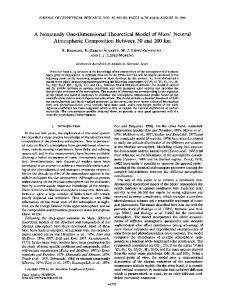
Lk Figure 2. Power spectra of u, plotted in coordinates that demonstrate inertial-range scaling, for the cases shown in table 1: ——, freely decaying turbulence; - - - -, bounded decaying turbulence; − . −, stationary turbulence.

To illustrate the performance of the simplest possible formulation of ODT, the three configurations are simulated without invoking small-eddy suppression. To assess the impact of this, the first configuration is also simulated with small-eddy suppression included. For the decaying cases, the sinusoidal initial profile is chosen for simplicity. After a transient interval, self-preserving decay is obtained that is insensitive to the functional form of the initial profile. The similarity scalings governing the decay are not considered in detail. The ODT scalings are found to be consistent with the scaling laws known to govern freely decaying turbulence (Chasnov 1994) and bounded decaying turbulence (Borue & Orszag 1995), except that ODT low-wavenumber spectra in the former case scale as k 2 rather than k 4 . This difference is a direct consequence of the one-dimensional formulation (Kerstein & McMurtry 1994b). Turbulence decay in ODT is therefore governed by slightly different scaling laws than those presumed to govern threedimensional flow; see Chasnov (1994) for a discussion of the relationship between low-wavenumber spectra and decay rates. 3.2.2. Spectral scalings: velocity −2/3 k 5/3 E(k). To test for inertial-range scaling, (3.1) is expressed in the form CK = 55 24 In figure 2, the right-hand side of this relation is plotted versus k in order to demonstrate the occurrence of the k −5/3 scaling, indicated by a plateau in the plot. For all three flows, the model parameter A is assigned the value 0.3, chosen to match the plateau level for the bounded decaying case to the measured value CK = 1.5 (Sreenivasan 1995). A determines the plateau level through the expression (B 1), or equivalently (B 2), for , where time and viscosity in those expressions depend on A as explained in § 2.5. A Reynolds number ReL = hu02 i1/2 L/ν is formed using the definition (B 6) of L. For simulations of each of the three homogeneous-flow configurations, values


ReL0 ReL ζ

Free decay 4600 330 1.67

Bounded decay 118 000 6720 1.67

295 Stationary 167 000 2000 1.73

Table 1. Computed inertial-range spectrum scaling exponents for three homogeneous flows.

of ReL corresponding to plotted spectra are shown in table 1. Also shown are nominal initial Reynolds numbers ReL0 of the simulated flows. For the decaying 1/2 flows, ReL0 = hu02 i0 L0 /ν. For the stationary flow, ReL0 = hdu/dyiY 2 /ν. After an initial transient, each of the simulated flows relaxes to the anticipated asymptotic behaviour: stationarity for the stationary case and self-similar decay for the other cases. For the stationary case, spectral and other statistical quantities are accumulated continuously after transient relaxation is completed. For the free and bounded decaying cases, self-similar decay begins at ReL = 500 and 7000 respectively. Table 1 indicates the values of ReL corresponding to the results shown in figure 2, which are based on order 103 simulated realizations. Figure 2 indicates a larger dynamic range of k −5/3 scaling for bounded decay than for free decay, owing to the large ReL value for the former. For the same A value, these two cases give the same CK . Numerical results for the exponent ζ in the scaling E(k) ∼ k −ζ are presented in table 1. The Kolmogorov scaling ζ = 53 is obeyed for the decaying flows but the stationary flow obeys power-law scaling with a different value of ζ. It has been noted that departures from Kolmogorov scaling may be obtained in simulations of forced stationary turbulence, possibly associated with intermittency induced by the forcing (Borue & Orszag 1995). The ODT simulation of stationary turbulence involves an arbitrary eddy-size cutoff l < Y that has no direct physical analogue. These observations do not fully resolve the status of the inertial-range scaling behaviour of ODT, but it can be stated that Kolmogorov scaling is obtained for the physically realizable cases that have been simulated. The inference in § 3.1.2 that the Kolmogorov microscale η marks the transition from inertial to viscous dominance is tested by plotting spectra in universal dissipationrange coordinates. Figure 3 shows that dissipation-range collapse of spectra is obtained for all three homogeneous flows, including the stationary flow that deviates from ζ = 53 in the inertial range. Comparison to figure 2 indicates the high sensitivity of the figure 2 format to small deviations from k −5/3 scaling. A curve representing the dissipation-range rolloff of measured spectra is also shown. This curve was obtained by fitting She’s analytical form (Sirovich et al. 1994) to a compilation of measured one-dimensional spectra (Monin & Yaglom 1975) and then applying the transformation (B 5) analytically to obtain the transverse spectrum directly comparable to ODT spectra. As noted in Appendix B, a given energy dissipation rate corresponds to a larger mean-square velocity cross-derivative in ODT, based on (B 2), than in threedimensional flow. Because the dominant contribution to is from the highwavenumber end of the inertial range, this implies an extension of the ODT inertial range to larger ηk than in three-dimensional flow, as seen in figure 3. The k −5 scaling derived in § 3.1.2 for the far-dissipation range of ODT is not seen in this figure, but it is seen in lower-ReL simulations that resolve more of the viscous range.

296

A. R. Kerstein 104

103

(η/ν 2)E

102

101

100

10–1

10–2 –3 10

10–2

10–1

ηk

100

101

Figure 3. Power spectra of figure 2, replotted in universal dissipation-range coordinates; − . . . −, measured spectrum. Line segment indicates k −5 scaling.

(ηε)–2/3kE *θ

101

100

10–1 –3 10

10–2

10–1

Pr –1/2ηk

100

101

Figure 4. Power spectra of scalars in bounded decaying turbulence at ReL = 2040, rescaled as explained in the text, plotted in universal high-wavenumber coordinates based on classical high-P r theory, for P r = 1 (− . . . −), 20 (− . −), 40 (- - - - -), and 80 (——). Line segment indicates k −5/3 scaling.

3.2.3. Spectral scalings: advected scalars As explained in § 3.1.3, the u profile can be interpreted as a passive-scalar field with P r = 1. The viscous-convective scaling in ODT is investigated by comparing this scalar to other passive-scalar fields with P r 1, subject to the same initial and boundary conditions as u. Results for the bounded decaying case are plotted in figure 4 in coordinates that


297

collapse the viscous-diffusive range kLB 1 according to the high-P r scaling analysis of § 3.1.3. The coordinates are defined so that 1/k spectral scaling corresponds to a plateau in the figure. The vertical axis is (η)−2/3 kEθ∗ , where Eθ∗ = (1 /θ )Eθ . (1 = /3 is the dissipation of the P r = 1 scalar.) Owing to the large dynamic range required to span the spectral ranges of interest, results are shown for ReL = 2040, lower than the ReL value of table 1 for this flow. ReL0 for this computation is the same as in table 1, but the results of figure 4 correspond to a later stage of decay than the bounded-decay results of figure 2. Lower ReL gives larger η and therefore more dynamic range allocated to the viscous regime. For the P r range shown in the figure, neither the viscous-convective spectral scaling nor the high-wavenumber collapse is fully attained. For the highest P r shown, Eθ ∼ k −1.1 at the inflection point of the plotted curve. In the dissipation range, the two intermediate-P r curves suggest an approach to collapse, but the highest P r does not maintain this trend. The slight flare at high wavenumbers for the highest P r suggests aliasing caused by inadequate spatial resolution, so the apparent deviation from dissipation-range collapse may be a numerical effect. Nevertheless, it is evident that the computed results are broadly consistent with the classical high-P r spectral scaling properties. 3.2.4. Freely decaying turbulence Aspects of freely decaying turbulence are considered in § 3.2.1 and § 3.2.2. This flow is revisited for three reasons. First, small-eddy suppression is introduced in order to assess its impact on computed results. (All subsequent computations include small-eddy suppression.) Second, the isotropy condition (§ 2.5) is used to determine A, thereby eliminating the need for empirical input to determine A. Third, a procedure for determining the initial u profile corresponding to a turbulence-generating grid is formulated. This procedure introduces no empiricism. The predicted decay of grid turbulence, obtained computationally in this manner, is compared to experimental results. In figure 5, the spectrum of figure 3 is replotted, along with two spectra from an identical computation, except that small-eddy suppression has been introduced. As in figure 3, the plotted results are based on A = 0.3, for which the measured value of the Kolmogorov constant CK is reproduced. A slight but discernible effect on the shape of the spectrum is seen at the high-wavenumber end of the inertial range. The two curves based on the new formulation collapse in accordance with dissipation-range scaling. The computation that includes small-eddy suppression is reinterpreted in the context of grid turbulence. The decay of velocity fluctuations in grid turbulence is considered. For this purpose, the isotropy condition hu02 i = hv 02 i is more relevant than the numerical value of CK . Enforcement of this condition in the self-similar decay regime of the simulation gives A = 0.82. As noted in § 2.5, the present formulation of ODT is not designed to reproduce all turbulence properties of interest with quantitative accuracy for a given A value. It is also noted in § 2.5 that a change of A value implies a rescaling of the Reynolds number associated with a given simulation. For A = 0.82, the simulation Reynolds number is ReL0 = 1680 rather than the value indicated in table 1. The initial velocity profile is u(y, 0) = u0 sin(2πy/L0 ), with L0 set equal to the mesh spacing M of the turbulence-generating grid, and u0 is chosen so that the u variance u20 /2 of u(y, 0) is equal to a simple estimate of the variance of u in the plane of

298

A. R. Kerstein 103

102

(η/ν 2)E

101

100

10–1

10–2 10–3

10–2

10–1

ηk

100

101

Figure 5. Computed power spectra of u in decaying homogeneous turbulence, plotted in universal dissipation-range coordinates. (η = (ν 3 /)1/4 is the Kolmogorov microscale.) ReL = 140 (- - - - -), 260 (——–), and 330 (− . −), where ReL = hu02 i1/2 L/ν, based on L = hu02 i3/2 /. The ReL = 330 curve, replotted from figure 3, is from a simulation that omits small-eddy suppression. The other curves are from a simulation that incorporates small-eddy suppression. A line segment of slope − 53 identifies the inertial range.

the grid. An estimate rather than a measured value is used in order to avoid the introduction of empiricism. Denoting the grid solidity as S, it is assumed that the flow in the grid plane consists of an area fraction S for which u = 0 and a fraction 1 − S for which u has the constant value U/(1 − S), chosen so that the mean flow in the grid plane matches the mean flow U in the homogeneous region downstream of the p grid. This gives a grid-plane u variance U 2 S/(1 − S) and thus u0 = U 2S/(1 − S). For the experiments considered here, S = 0.34. Computational time is converted to streamwise distance using the relation x = Ut. Figure 6 compares the computed decay of u and v variance to empirical far-field correlations (Yoon & Warhaft 1990) for decaying grid turbulence. It is seen that reasonable quantitative agreement is obtained over the streamwise range of typical grid-turbulence experiments (ranging up to x/M of several hundred), despite the complicated near-field behaviour of this flow. The persistent small-scale anisotropy of this flow, reflected in the empirical correlations, is not reproduced because isotropy has been deliberately enforced. This ODT grid-turbulence model may be useful for addressing aspects of grid turbulence, and passive-scalar mixing therein, that have been examined experimentally. In this regard, the artifact discussed in Appendix A is relevant. Namely, large eddies with τ values greatly exceeding the elapsed time t occur infrequently in ODT, but their effect on transport is disproportionate. In particular, the root-mean-square (r.m.s.) fluctation of a scalar with non-zero mean gradient is determined by the scalar displacements in the gradient direction, and hence is sensitive to this anomalous transport. Consequently, it is found in ODT grid-turbulence simulations with an imposed scalar gradient that the streamwise profile of the scalar r.m.s. fluctuation exceeds the measured profile by roughly a factor of six, based on the empirical


299

〈u′2〉/U 2, 10 × 〈v′2〉/U 2

10–2

10–3

10–4

10–5 101

102

103

x/M Figure 6. Computed evolution of streamwise and transverse velocity variance in decaying grid turbulence: − . −, streamwise variance; − . . . −, transverse variance. Empirical correlations (Yoon & Warhaft 1990): ——–, hu02 i/U 2 = 0.0712(x/M)−1.31 ; - - - - -, hv 02 i/U 2 = 0.0652(x/M )−1.34 .

correlation in figure 10 of Yoon & Warhaft (1990). Anomalous dispersion of scalars released from localized sources is likewise anticipated. This issue has been addressed in detail in the context of the LEM (Kerstein 1991, 1992; de Bruyn Kops & Riley 1998).

4. Wall-bounded flow ODT simulations of Couette flow, channel flow, pipe flow (based on a cylindrical formulation not presented here), and the spatially developing planar boundary layer have been performed. Results are presented here for Couette flow, because it is the base case for stratified boundary-layer problems considered in § 6. Couette flow is simulated by applying the boundary conditions u(0, t) = 0, u(Y , t) = U to the computational domain [0, Y ]. The initial velocity profile is linear, but this is immaterial because only the statistically steady flow that follows transient relaxation is considered. Following convention, this flow is characterized by the half-width Reynolds number Re = UY /(2ν). The model parameter A is assigned the value 0.23 because this value is found to give a good match to the friction law and growth law of the spatially developing planar boundary layer. (Results for this flow are not presented here.) With this choice, Couette-flow results are compared to measurements without introducing additional empiricism. Computed results are shown for Re = 2900 and 18 000, values for which Reichardt measured mean velocity profiles in Couette flow. Computed results are compared to his measurements, reported by Schlichting (1979), in figure 7. Reasonable overall agreement is obtained. The computed mean velocity profiles are replotted in wall coordinates in figure 8. (Here, u+ = hui/uτ and y + = yuτ /ν, where uτ = (νdhui/dy|y=0 )1/2 is the friction velocity.) Precise collapse of the wall-scaled profiles is obtained, with a wide zone

300

A. R. Kerstein

〈u〉/U

1.0

0.5

0

0.5

1.0

y/Y Figure 7. Mean velocity profiles in Couette flow. Computations: Re = 2900 (——–), 18 000 (- - - - -). Measurements by Reichardt (Schlichting 1979): Re = 2900 (), 18 000 (4). 25

20

15

u+ 10

5

10–1

100

101

102

103

y+ Figure 8. Computed mean velocity profiles of figure 7, replotted in wall coordinates. Also plotted are the functions u+ = 3.8 ln y + − 1.5 (——–) and u+ = y + (− . −) that identify the log-law and viscous layers, respectively.

of logarithmic dependence. The log-region scaling corresponds to a value κV = 0.26 ´ an ´ constant, close to the value 0.25 obtained from the spatially of the von Karm developing boundary-layer simulation. The measured value is 0.41 (Hinze 1975). The conformance of the computed results to familiar scaling properties of the boundary layer stems largely from the fact that these properties can be derived from momentum conservation in conjunction with fairly mild assumptions concerning


301

〈v′2〉1/2/uτ

1.0

0.5

0 10–1

100

101

102

103

y+ Figure 9. Transverse-velocity fluctuation profiles computed for Couette flow: Re = 2900 (——–), 18 000 (- - - - -). Measurements in channel flow (Wei & Willmarth 1989): Re = 2970 (4), 14 914 ().

the structure of the near-wall and outer flows. These assumptions should be no less applicable to ODT than to three-dimensional turbulence. Nevertheless, it is noteworthy that ODT reproduces diverse facets of boundary-layer phenomenology within a simple modelling framework. The computed profiles of hv 02 i1/2 , plotted in wall coordinates, are compared to channel-flow measurements (Wei & Willmarth 1989) in figure 9. The model underpredicts the peaks of the measured profiles roughly to the same extent that it underpredicts peaks of hu02 i1/2 /uτ profiles (not shown). Thus, the model is internally consistent in its representation of u and v fluctuations, lending support to the formulation of v fluctuation statistics in Appendix C. The degree of predictive accuracy indicated by figure 9 is typical of second-order fluctuation statistics computed for wall-bounded flows. In figure 10, computed terms of the budget of hu02 i/2 for Re = 2900 are compared to the turbulent kinetic energy budget from channel-flow DNS at Re = 3300 (Mansour, Kim & Moin 1988). (hu02 i/2 is the model analogue of turbulent kinetic energy in boundary-layer flows, as explained in Appendix C.) Comparisons by Mansour et al. (1988) and by Eggels et al. (1994) of the channelflow results to results for the planar boundary layer and for pipe flow indicate that the near-wall energy balance is insensitive to flow configuration. Channel DNS at Re = 7900 (Antonia et al. 1992) indicates slight increases of the production peak and of the near-wall dissipation relative to the Re = 3300 results. The DNS results are plotted on the negative y + -axis for ease of comparison. The computed terms of the balance, based on (C 6), are expressed in wall coordinates by normalizing by u4τ /ν. In this plot, the scaling of the horizontal coordinate depends on A, but the height of the profiles does not. The ODT energy balance is seen to be in fairly good quantitative as well as qualitative agreement with the DNS energy balance. This is possible only because pressure transport is a minor contribution to the energy balance in the boundary

302

A. R. Kerstein 0.3

Gain

0.2

0.1

0

Loss

–0.1

–0.2

–0.3 –50

–25

0

25

50

y+ Figure 10. Computed near-wall turbulent kinetic energy balance in Couette flow based on ODT for Re = 2900 (positive y + ), and in channel flow based on DNS for Re = 3300 (Mansour et al. 1988; negative y + ): ——–, production (upper curve), dissipation (lower curve); - - - - -, turbulent transport; − . −, viscous transport; − . . . −, pressure transport (DNS only; ODT has no pressure-transport mechanism).

layer, so its omission from ODT does not impose large perturbations on the other terms. Numerous second-order closures, reviewed by So et al. (1991), have been proposed for near-wall turbulence. Several of them provide better overall representations of one-point statistics up to third order than does ODT. This comparison is noted in order to emphasize that the simple approach adopted here is neither designed nor intended to outperform models tailored to reproduce the low-order one-point statistics of particular flows. The present goal is to capture diverse features of many flows within a unified framework that allows straightforward extension to variableproperty flows, reacting flows, and related problems. This addresses both the scientific goal of conceptual unification and the practical objective of reliably extrapolating from constant-property conditions to engineering problems involving many strongly coupled physical processes.

5. Buoyancy-driven flow 5.1. Homogeneous buoyancy-driven turbulence As noted in § 2.4.1, (2.14) implies a simple method for simulating buoyancy-driven turbulence with no applied shear. The u profile is omitted entirely, yielding self-driven density-profile evolution (DPE). All flows considered in § 5 are simulated in this manner. In buoyancy-driven turbulence, as in shear-driven turbulence, the most fundamental property is the eddy cascade. The buoyancy-driven cascade is not as well understood as the shear-driven cascade. Detailed assessments of recent theoretical and experimental work are provided by Grossmann & L’vov (1993) and by Siggia (1994). Procaccia & Zeitak (1989) proposed that the temperature spectrum measured by Wu


303

et al. (1990) in buoyancy-driven turbulence could be interpreted as a manifestation of the Bolgiano–Obukhov (BO) scaling, originally predicted to occur in stably stratified turbulence. L’vov (1991) noted that the locality of interactions between eddies and density fluctuations implies that scaling in the buoyancy-dominated wavenumber range should be indifferent to the direction of the stratification. Various analytical and computational models of buoyancy-driven turbulence have subsequently reproduced the BO scaling. Here, a scaling analysis is developed that reflects the presumed governing mechanism. The analysis is based on the features of buoyancy-driven turbulence that are incorporated into ODT, thereby identifying the origin of BO scaling within the ODT framework. Density fluctuations are assumed to cascade toward high wavenumbers due to mapping-induced reduction of fluctuation length scales. Because mappings conserve all scalar properties, this cascade conserves the spectral intensity of density fluctuations, denoted ρ2k , at wavenumbers k below the wavenumber range (identified shortly) in which molecular diffusion is significant. Assume, subject to self-consistent verification, that the cascade time scale τk decreases with increasing k, so that the high-k cascade equilibrates rapidly with respect to low-k transients. A quasi-steady analysis can then be applied. In a quasi-steady cascade that conserves ρ2k , the flux of ρ2k to higher k is of order 2 ρk /τk and is independent of k, giving ρ2k ∼ τk . (In this and subsequent scaling analyses, numerical coefficients are omitted.) The power spectrum Eρ (k) of density fluctuations, which scales dimensionally as ρ2k /k, is determined by ρ2k ∼ τk and one additional relation involving ρk and τk . The additional relation follows from (2.14) and (2.15), specialized to DPE. For l = 1/k, the density difference in the integrand of (2.15) is of order ρk and the y dy-integration introduces an additional factor of k −2 . Equation (2.14) then gives ρ0 /(kτk )2 ∼ ρk /k. In conjunction with ρ2k ∼ τk , this gives ρk ∼ k −1/5 and thus Eρ (k) ∼ k −7/5 , which is the BO scaling of the density spectrum. This result may be interpreted as follows. Equation (2.14) implies that size-l eddies are driven by density fluctuations of comparable size. This locality property of the buoyancy-driven cascade, analogous to the presumed locality of the inertial cascade, has been proposed as the mechanistic basis of the dimensional relations underlying the BO scaling (L’vov 1991). Because kinetic energy is not explicit within DPE, DPE cannot address the possibility that the kinetic-energy cascade, rather than the density cascade, governs buoyancydriven turbulence. Evidence supporting this possibility is discussed by Siggia (1994). To derive crossovers from BO scaling to other scaling regimes, consider the following initial-value problem for ODT. A constant, unstable density gradient is imposed initially on a size-Y domain. Jump-periodic boundary conditions, as defined in § 3.2.1, are applied in order to emulate an imposed density gradient on an unbounded domain. Mappings larger than Y are disallowed. This restriction is arbitrary from a physical viewpoint, but convenient for deriving and computationally demonstrating scalings of interest. A large-k crossover to a regime dominated by molecular transport occurs at a wavenumber such that the eddy time scale τk is comparable to the smaller of the two molecular time scales 1/(k 2 ν) and 1/(k 2 κ). Consider P r 6 1, for which the latter is smaller. Substituting earlier results into τk ∼ 1/(k 2 κ), the scaling Y kB ∼ (RaP r)5/16 is obtained for the crossover wavenumber kB , where Ra is based on the length scale Y . For P r 6 1, the density spectrum is suppressed at k above kB by molecular dissipation of density fluctuations. In three-dimensional flow with P r < 1, velocity

304

A. R. Kerstein

fluctuations at k above kB cascade from wavenumber kB , at which they are driven by density fluctuations, to a higher-k cutoff at which they are suppressed by viscous dissipation. This cascade is governed by the usual inertial-range dynamics, giving k −5/3 scaling of the energy and density spectra in this subrange (Grossmann & L’vov 1993). In DPE, there is no mechanism other than density fluctuations to drive fluid motions. For k greater than kB but below the viscous cutoff, scaling analysis of DPE (details omitted) gives k −9/2 scaling of the density spectrum. In contrast, for sheardriven stably stratified flow, ODT captures the inertial-range dynamics leading to the k −5/3 subrange, for the same reasons that ODT captures this subrange in non-buoyant flow. For P r > 1, analogous considerations give Y kB ∼ (Ra/P r)5/16 , where kB is now the viscous cutoff. Eddies are suppressed at k above this cutoff, but density fluctuations persist up to a higher wavenumber corresponding to the molecular-diffusive cutoff. The subrange between these cutoffs is a viscous-convective subrange with respect to density, so 1/k scaling of the density spectrum is anticipated (Lesieur 1990). DPE as well as shear-driven ODT captures the mechanism that causes this scaling. For any P r, eddies and density fluctuations are suppressed at sufficiently high k. Scaling analysis (details omitted) indicates that the high-k falloff of the density spectrum is faster than power law but slower than exponential. This behaviour is qualitatively consistent with current understanding of the far dissipation range (Sirovich et al. 1994). The BO scaling predictions and the predicted scaling of kB agree with the predictions of L’vov (1991), reflecting the fact that DPE and L’vov’s analysis are both predicated on the locality of the buoyancy-driven cascade. Procaccia & Zeitak (1989) derived the BO scaling from a different viewpoint, obtaining a different scaling of kB . Measurements by Tong & Shen (1992) confirm L’vov’s prediction, lending support to the locality principle underlying his analysis and DPE. These predictions (except P r dependences) are tested by simulating the imposeddensity-gradient configuration with maximum event size Y for two Ra values with P r = 1. Figure 11 shows density spectra (defined in accordance with the scalar spectrum formulation in Appendix B) determined from the statistically steady evolution of this configuration after transient relaxation. The axes are scaled to demonstrate the Ra5/16 scaling of kB . It is seen that the BO spectral scaling and the anticipated Ra dependence of kB are obeyed. In conjunction with the results of § 3, it is thus demonstrated that (2.14) encompasses the physics governing both the inertial cascade and the buoyancy-driven cascade, and thereby provides an opportunity for future study of cascades in mixed convection. 5.2. Rayleigh convection 5.2.1. Heat-transfer analysis The structure of statistically steady convection between horizontal plates, driven by thermal boundary conditions applied at the plates, is of considerable practical importance and raises scientific issues at the frontier of turbulence research (Siggia 1994). Heat transfer in this flow is the key issue, both from a practical and a fundamental viewpoint. Heat transfer is also a convenient focal point for a general discussion of Rayleigh convection. Therefore the dependence of the Nusselt number Nu on Ra and P r is considered, where Nu is the mean heat flux divided by the heat flux in the absence of fluid motion. In statistically steady convection, the mean heat flux is independent of y between the


305

Ra7/16Y –3(d〈 ρ〉/dy) –2Eρ

102

100

10–2

10–4

10–3

10–2

10–1

100

101

Ra –5/16Yk Figure 11. Computed power spectra of density fluctuations in stationary homogeneous buoyancy-driven turbulence, normalized to demonstrate the scaling of the high-wavenumber cutoff, for P r = 1: ——–, Ra = 1011 ; - - - - -, Ra = 1012 . A line segment of slope − 75 identifies the Bolgiano–Obukhov scaling regime.

plates, so it is equal to −κdhT i/dy|y=0 , the heat flux at the lower plate. (Here, plates are located at y = 0 and L. The factor ρ0 c is omitted because it drops out of all normalized fluxes, assuming constant heat capacity c.) In motionless fluid, dhT i/dy is equal to −∆/L for all y, where ∆ is the magnitude of the imposed temperature difference, and the heat flux is κ∆/L. These relations give L dhT i . (5.1) Nu = − ∆ dy y=0 In DPE, Rayleigh convection is simulated by maintaining an unstable density difference across the y interval [0, L]. In the Boussinesq approximation, density and temperature differences are proportional, but opposite in sign, so the thermal interpretation of this configuration follows directly. In normalized units, this flow is characterized by Ra and P r. The dependence of Nu on Ra and P r in DPE is considered. This dependence is sensitive to several features of wall-bounded buoyancy-driven flow in DPE. The key assumption in the classical similarity analysis of Rayleigh convection is that near-wall flow structure is independent of plate separation L for large Ra. The mixing-length similarity scalings that follow from this assumption explain many features of Rayleigh convection and related flows (Adrian et al. 1986; Siggia 1994). However, nonclassical scalings attributed to bulk-flow effects are observed in some high-Ra flow regimes (Siggia 1994). As in three-dimensional Rayleigh convection, it is anticipated that mixing in the interior of the DPE simulation suppresses the mean density gradient, which therefore resides primarily in conduction-dominated wall layers. This picture is verified selfconsistently through scaling analysis, supported by numerical results. The focus of the scaling analysis is estimation of the thickness yκ of the conduction layers. In particular, the possible dependence of conduction-layer structure on L is considered.

306

A. R. Kerstein

The thickness yκ is determined by the balance of diffusive broadening of the layers and advective transfer of wall-layer fluid to the interior. Layer broadening and erosion may be visualized as a renewal process in which the layer grows diffusively until advective disruption occurs, followed by regrowth. Diffusive scaling implies yκ2 ∼ κtκ , where tκ is the characteristic disruption time. Though this picture of successive disruptions is reminiscent of the periodic generation of thermals observed in convection at moderate Ra (Sparrow, Husar & Goldstein 1970), neither the model nor its interpretation relies on a direct correspondence between individual events within the simulation and observed fluid motions. The performance of the model reflects the scalings governing the ensemble of simulated events. For estimation purposes, a disruption is defined as a mapping of size yκ or larger whose closest approach to the wall is less than yκ . Then tκ is the mean time between such events. In principle, mappings smaller than yκ may affect the scaling, e.g. through their contribution to an eddy diffusivity κe > κ governing diffusive-layer growth. However, it follows from the ensuing analysis that mappings smaller than yκ can occur in DPE only if P r < 1, and that κe is of order κ in this P r range. Thus, large events (l > yκ ) determine tκ . Small events (l < yκ ) enhance diffusive growth of the conductive layer, but not enough to affect scalings. Consider the mean time tκ (l) between disruptions by mappings of characteristic size l > yκ . For estimation purposes, each mapping is deemed to redistribute fluid from the zone [0, yκ ] uniformly throughout [0, l]. (For clarity, the lower layer is considered here.) Therefore (2.15) gives ∆Eg ∼ g∆ρyκ l, where ∆ρ is the imposed density difference across [0, L]. (For high Ra, roughly half of this density difference resides √ within each wall layer.) Equation (2.14) then gives the l-eddy time scale τl ∼ l/ g 0 yκ , where g 0 denotes g∆ρ/ρ0 . To express tκ (l) in terms of τl , note that (2.2) determines the event-rate distribution λ in terms of l and τl . The event rate for order-l eddies with 0 6 y0 6 yκ can be estimated by dl-integration of λ over [l, 2l] and dy0 -integration over [0, yκ ]. This gives the rate of order-l disruption events, p whose inverse is the disruption time scale tκ (l). Thus, tκ (l) ∼ lτl /yκ , giving tκ (l) ∼ l 2 / g 0 yκ3 . Now, tκ is taken to be the smallest tκ (l) such that l > yκ . In the absence of viscous effects, this gives tκ = tκ (yκ ). However, viscosity is implemented in DPE by disallowing √ events for which τl > l 2 /(16ν). The smallest allowed event is therefore of size yν ∼ ν/ g 0 yκ . It follows from the ensuing solution for yκ that this minimum size exceeds yκ only for P r > 1. Therefore P r > 1 and P r 6 1 are considered separately. (Owing to numerical coefficients omitted from the scalings, the crossover between P r regimes actually occurs at non-unity P r; see § 5.2.2.) For P r > 1, tκ = tκ (yν ) is evaluated in the relation yκ2 ∼ κtκ to obtain, after some manipulation, yκ ∼ (κν 2 )2/9 /g 01/3 . The estimate Nu ∼ L/yκ , based on (5.1) and the order-∆ temperature drop in the yκ -layer, gives Nu ∼ Ra1/3 P r−1/9 ,

(5.2)

where Ra is given by (2.18). For P r 6 1, tκ = tκ (yκ ). This gives yκ ∼ (κ2 /g 0 )1/3 and thus Nu ∼ (RaP r)1/3 .

(5.3)

Equations (5.2) and (5.3) necessarily conform to the mixing-length scaling Nu ∼


307

f(P r)Ra1/3 , which follows from the assumed insensitivity of near-wall behaviour to L (Siggia 1994). Support for this assumption in the present context is provided shortly. The P r dependence in (5.3) is simply a reflection of the irrelevance of the viscosity in the low-P r limit. The P r dependence in (5.2) follows from the suppression of fluid motions below the viscous cutoff in DPE. A more complete high-P r theory that accounts for viscous-scale fluid motions (Kraichnan 1962) gives Nu ∼ Ra1/3 , independent of P r. Measurements suggest that neither this result nor (5.2) is entirely accurate. (Kraichnan notes that a key assumption in his theory is unlikely to be strictly correct.) Evidence that Nu is an increasing function of P r for high P r is noted shortly. A corollary of the derivation of (5.2) is the relation yν /yκ ∼ P r1/3 for high P r. In contrast, Kraichnan’s theory predicts that this ratio of viscous-layer and thermal-layer thicknesses scales as P r1/2 for high P r. A complication that may affect the Ra as well as the P r dependence is the occurrence of large-scale interior flows in some high-Ra convection regimes (Siggia 1994). The proposed governing mechanisms involve flow phenomena that are not represented within DPE. Nevertheless, DPE results may have some bearing on measured Nu scalings that have been attributed to these phenomena. Before examining the computed results, large-scale effects in the DPE formulation of Rayleigh convection are analyzed. Only P r > 1 is considered because all properties of interest are independent of P r for low P r. As noted earlier, this insensitivity is shown by comparing κ to the eddy diffusivity κe of mappings of size yκ or less contained within [0, yκ ]. Straightforward extension of the foregoing analysis gives κe ∼ yκ2 /τκ , and consequently κe ∼ κ, for low P r. This establishes the claimed insensitivity to P r for low P r, so only P r > 1 is considered in the remainder of the analysis. At high Ra, the large-scale flow is characterized by L and the potential energy input rate Nu κg∆ρ/L ∼ κg∆ρ/yκ . In steady state, the energy input equals the kinetic energy dissipation rate, of order ρ0 v 3 /L, where v is a characteristic large-scale velocity. This is equivalent to the usual analysis based on the heat flux driven by the imposed temperature difference (Adrian et al. 1986), but is more direct for purposes of flow analysis. Then v ∼ (κg 0 L/yκ )1/3 . The large-scale flow governs the wall-layer thickness yκ , and thus Nu, only if it disrupts the wall layer on a time scale shorter than the time scale tκ determined by considering only the near-wall flow. The large-eddy time scale is τL ∼ L/v. As in the analysis of wall-layer disruption by size-l eddies, τL is multiplied by L/yκ to obtain the time scale for disruption of the wall layer by large eddies. Combining results thus far, it is found that large-scale flow dominates only for Ra < P r17/15 . For given P r, large-scale effects are negligible at sufficiently high Ra. Thus, DPE does not capture the transition back to large-scale dominance at exceedingly high Ra that was predicted by Kraichnan (1962) and possibly observed in a recent experiment (Chavanne et al. 1997). 5.2.2. Heat-transfer results Rayleigh convection is simulated in DPE by choosing an arbitrary initial density profile, applying constant-density boundary conditions at y = 0 and y = L with ρ(0) < ρ(L), and running the simulation until transients are relaxed before gathering statistics. Heat-transfer properties based on simulations performed for various Ra and P r values are shown in figures 12 and 13. Figure 12 is scaled so that, for given P r, (5.2) corresponds to no dependence of the

308

A. R. Kerstein

Ra –1/3Nu

10–1

10–2 105

106

107

108

109

1010

Ra Figure 12. Heat transfer in Rayleigh convection, using high-P r scaling. Computations: , P r = 10; , P r = 100; 4, P r = 1000; ∗, P r = 10 000. Dashed lines are separated by factors of 101/9 . Measurements: lower solid line, P r = 6.5 (Goldstein & Tokuda 1980); upper solid line, P r = 2750 (Goldstein et al. 1990).

plotted quantity on Ra. It is seen that the Ra1/3 scaling of Nu is obeyed for Ra > 107 . Results for P r = 10, 100, 1000 and 10 000 are shown. The dashed lines are separated by factors of 101/9 to indicate the vertical displacement between successive P r values that is prescribed by (5.2). The anticipated P r dependence is obtained for P r > 100. The solid lines represent the Ra1/3 scaling of Nu inferred by Goldstein & Tokuda (1980) from measurements at P r = 6.5 (lower line), and by Goldstein, Chiang & See (1990) from measurements at P r = 2750 (upper line). Their results indicate a slight increase of Nu with increasing P r. Earlier measurements (Globe & Dropkin 1959) indicate the same trend, with stronger P r dependence (Nu ∼ P r0.074 ). It appears that DPE as presently formulated gives fairly accurate heat-transfer results for P r of order 10 (corresponding to Rayleigh convection in water), with increasing deviation from measured results as P r increases. Results for P r ranging from 0.01 to 10 are plotted in figure 13. The scaling is chosen so that the data should collapse on a horizontal line if (5.3) is obeyed. The anticipated P r dependence is seen for P r below 0.1. High-Ra onset of the anticipated Ra dependence is apparent, though the results are not definitive in this regard. Figures 12 and 13 indicate that the transition between high-P r and low-P r scaling occurs near P r = 10. Experiments, however, indicate that the transition occurs near P r = 0.1 (Siggia 1994). As noted in § 2.4.1, the P r value in DPE is governed by smalleddy suppression. The suppression criterion involves a somewhat arbitrary numerical factor (Appendix A) that could in principle be adjusted to match the P r value at which the transition between scalings is observed. Empirical adjustments of this sort are useful for obtaining quantitatively accurate, calibrated models of particular flows, but are not attempted here. In the DPE results and in measurements, transitional Ra dependences of Nu are seen for P r of order unity or less. Summarizing their own and previous measurements,


309

(Ra Pr) –1/3Nu

10–1

10–2 104

105

106

107

108

109

1010

Ra Pr Figure 13. Heat transfer in Rayleigh convection, using low-P r scaling. Computations: ◦, P r = 0.01; 5, P r = 0.1; ×, P r = 0.7; +, P r = 1; , P r = 10. Line segments: - - - - -, Nu ∼ Ra1/4 ; ——–, Nu ∼ Ra2/7 .

Cioni, Ciliberto & Sommeria (1997) conclude that the power of Ra appearing in the Nu scaling is 0.26 at low P r, near 27 at P r of order unity, and near 13 at high P r. Large-scale motions are observed that depend on vessel shape and on P r, but at P r of order unity, the suppression of these motions by screens does not change the heat-transfer scaling. Cioni et al. (1997) note the difficulty of reconciling these and other observations with various models that have been proposed. The models typically involve the application of mixing-length concepts to a proposed schematic picture of the flow. The models for different regimes bear no obvious relation to each other. It is interesting in this regard that DPE exhibits significant (two decades or longer) transitional Nu scalings that are consistent with the 0.26 and 27 exponents seen at low and moderate P r respectively. Also consistent with measurements is the robustness of Ra1/3 scaling at high P r. The DPE results for low P r are especially interesting because they indicate Nu ∼ Ra1/4 transitional scaling and also indicate a Re scaling that is consistent with measurements (§ 5.2.4). In contrast, a low-P r mixing-length analysis that reproduces Nu ∼ Ra1/4 scaling disagrees with the measured Re scaling (Cioni et al. 1997). Thus, DPE reconciles a variety of behaviours that have not previously been explained within a single framework. Application of mixing-length analysis to DPE itself does not explain the performance of the model. As shown in § 5.2.1, Nu ∼ Ra1/3 is predicted for all P r regimes of the DPE simulation. The additional transitional scalings seen in the DPE numerical results highlight the distinction between conventional mixing-length analysis and mixing-length physics as embodied in DPE (or more generally, in ODT). Equation (2.3) is a mixing-length relation applied to an individual eddy, rather than to an ensemble-averaged flow property. Owing to the strong two-way coupling between mapping events and the velocity profile, this formulation admits the possibility of flow evolution qualitatively different from

310

A. R. Kerstein

the evolution predicted by conventional mixing-length analysis applied to ensembleaveraged properties. The agreement between the heat-transfer regimes of DPE and measured behaviours suggests that DPE does in fact capture physics not described by conventional mixing-length analysis. The simplicity of the model suggests that the relevant physics is not specific to boundary-layer structure, large-scale flow, or plume development, all of which have been proposed as possible governing mechanisms (Siggia 1994; Cioni et al. 1997). 5.2.3. Thermal structure Profiles of moments of the temperature profile in Rayleigh convection have been obtained for P r = 0.7 from DNS (Kerr 1996). Analogous profiles are obtained from DPE simulations which have been performed for Ra and P r values corresponding to those of the DNS study. DPE and DNS values of scaling exponents governing the Ra dependence of features of these profiles are compared. Following Kerr (1996), the structure of the temperature variance profile is characterized by ∆c /∆, ∆w /∆, and λT /L, where ∆c is the centerline r.m.s. temperature fluctuation, ∆w is the peak r.m.s. fluctuation, and λT is the distance of the peak from the wall. Classical mixing-length theory predicts ∆c ∼ Ra−1/9 and λT ∼ Ra−1/3 , but an alternative mixing-length analysis predicts ∆c ∼ Ra−1/7 and λT ∼ Ra−2/7 (Castaing et al. 1989). DPE obeys both classical scalings although it obeys a non-classical Nu scaling in this parameter range (§ 5.2.2). The DNS results (Kerr 1996) do not clearly discriminate between the classical and non-classical scalings. Both DPE and DNS indicate that ∆w decreases more slowly with Ra than ∆c . Collectively, the thermal-structure and heat-transfer results indicate various transitional behaviours that are not readily subsumed within a conventional mixinglength picture. 5.2.4. Flow properties The principal characterization of flow as distinct from thermal properties of Rayleigh convection is the Reynolds number Re = vL/ν, where the characteristic velocity v is taken to be the r.m.s. vertical velocity fluctuation hv 02 i1/2 midway between the walls. The parametric dependences of Re are estimated using conventional mixing-length theory. It is assumed that the energy dissipation, of order ρ0 v 3 /L, is proportional to the potential energy input rate Nu κg∆ρ/L. This gives the mixing-length prediction (Siggia 1994) (5.4) Re ∼ (NuRa/P r2 )1/3 for all P r. This relation is expressed in terms of Nu, rather than substituting a particular dependence of Nu on Ra and P r, so that it may in principle subsume all Nu scaling regimes. However, the scaling ρ0 v 3 /L assumed for the energy dissipation may not be applicable if the dissipation is governed by the interaction between a large-scale interior flow and the wall layer. Siggia (1994) shows that near-sidewall velocity measurements for P r near unity deviate from (5.4) in a manner that suggests such an interaction. DPE lacks the mechanism that causes this deviation. Accordingly, figure 14 shows that the DPE results obey (5.4) over the entire range of P r and Ra spanned by the simulations, except for possible low-Re deviations. Also plotted in figure 14 are experimental and numerical data correlations. The DNS results of Kerr (1996) for P r = 0.7 suggest a departure from the Ra dependence


311

105

104

103

Re 102

101

100 100

101

102

(Nu

103

104

105

Ra/Pr 2)1/3

Figure 14. Computed Re in coordinates based on mixing-length theory. Symbols as in figures 12 and 13; - - - - -, linear fit to computed results. Correlations inferred from measurements: ——–, P r = 0.7 (Fitzjarrald 1976); − . −, P r = 7 (Tanaka & Miyata 1980). − . . . −, correlation based on direct numerical simulation for P r = 0.7 (Kerr 1996). Correlations are plotted over the ranges of the respective data sets.

implied by (5.4), but interior-flow velocity measurements for P r = 0.7 (Fitzjarrald 1976) and P r = 7 (Tanaka & Miyata 1980) obey that Ra dependence. The P r = 7 result is obtained by assuming isotropy of the interior flow. The accuracy of this assumption was not checked, so the difference between the two measured correlations does not necessarily imply a deviation from the P r dependence of (5.4). A flow Reynolds number inferred from thermal time histories has also been found to obey (5.4) for given P r (Cioni et al. 1997). The ODT results and the comparisons to DNS and experimental results indicate that the definition of velocity in terms of the cell displacement and the event time scale in § 2.4.1 is consistent with the classical mixinglength theory of Rayleigh convection and yields reasonably accurate quantitative results. 5.3. Penetrative convection A key feature of atmospheric-boundary-layer (ABL) dynamics is the daytime growth of the buoyancy-driven mixed layer as it penetrates the stably stratified layer established earlier by nocturnal surface cooling (Stull 1988). Deardorff’s (1970) convective scalings have been used to correlate a variety of laboratory and field measurements and numerical simulations of mixed-layer structure (Adrian et al. 1986; Coleman & Ferziger 1996). The correlations indicate that important features of the scaled structure are insensitive to Reynolds number, mean shear, Coriolis effects, and transient growth of the layer. Deardorff & Willis (1985) performed a shear-free penetrative-convection experiment that has become a benchmark for mixed-layer data correlations. Their configuration is an initially linear, stable thermal stratification, heated from below. In DPE, this configuration is simulated by applying a constant density flux −Q at the bottom of a linear, stable initial density profile characterized by the length scale

312

A. R. Kerstein 8

〈ρ( y) – ρ(0)〉/ρw

6

4

2

0

–2

–4

0

500

1000

1500

2000

y/yw Figure 15. Computed mean density profiles in penetrative convection, referenced to the density at the wall, in wall coordinates, for P r = 6, Rem = 1544 (——–), 2044 (- - - - -), and 2488 (− . −).

L ≡ ρ0 /(dρ/dz). Computed results are normalized using either wall-layer (conduction) scalings vw = (gκQ/ρ0 )1/4 ,

yw = κ/vw ,

ρw = Q/vw

(5.5)

or mixed-layer (convection) scalings ym ,

vm = (gym Q/ρ0 )1/3 ,

ρm = Q/vm ,

(5.6)

where ym is a measure of mixed-layer depth (Adrian et al. 1986). The mixed-layer flow is characterized by P r and the Reynolds number Rem = vm ym /ν. Computations were performed for P r = 6, corresponding to the experimental conditions of Deardorff & Willis (1985), and also for P r = 1. Flow evolution was simulated until Rem = 2500 was reached. Coleman & Ferziger (1996) estimated that the typical Rem value for the Deardorff–Willis experiment was 2000. The collapse of conduction-scaled mean density profiles obtained from the P r = 6 simulations is shown in figure 15. A slight unstable stratification is seen in the mixed layer, but Deardorff & Willis (1985) obtained a slight stable stratification. Away from the conduction layer, collapse of convection-scaled quantities is obtained for Rem above 1200, with one exception that is noted shortly. Plotted profiles correspond to Rem in the vicinity of 2000. The scaled flux profiles (density flux for the simulation, heat flux for the experiment) shown in figure 16 indicate almost uniform heating of the mixed layer, owing to the suppression of thermal gradients by turbulent transport. The profiles show flux reversal above the mixed layer, reflecting entrainment of fluid from the stable capping layer. The mixed-layer depth ym is defined as the y location of the most negative flux (Deardoff, Willis & Stockton 1980). The experiment indicates stronger flux reversal than the simulation. To assess how this affects the growth rate of the mixed layer, it is important to distinguish between entrainment and encroachment (Turner 1991). Encroachment is growth of


313

1.0

0.8

–〈ρ′v′〉/Q

0.6

0.4

0.2

0

–0.2

0

0.2

0.4

0.6

0.8

1.0

1.2

y/ym Figure 16. Computed (——) and measured (Deardorff & Willis 1985; symbols) vertical profiles of density flux, normalized by its wall value, for P r = 6. (Measured profile is the thermal analogue of this quantity.)

the near-constant-property layer caused by the influx of the conserved property at the boundary, irrespective of advection within the layer. A simple model of this process is obtained by assuming that ρ is independent of y in the mixed layer y < ym and has its initial, linear functional form for y > ym . For constant Q, this yields t1/2 growth of ym . The predicted growth is found to be in good numerical agreement with the computed evolution of ym . Analogous reasoning led Deardorff, Willis & Lilly (1969) to a good prediction of mixed-layer growth in their penetrative convection experiment. Thus, encroachment rather than advective entrainment appears to be the dominant growth process in this shear-free flow configuration, so differences between computed and observed rates of advective entrainment have little impact on the overall growth rate. The simplicity of this picture of mixed-layer growth is specific to penetrative convection. Shear-driven entrainment involves additional considerations that are examined in § 6.3. In figure 17, computed density-fluctuation profiles are compared to temperature fluctuations measured by Deardorff & Willis (1985). The computed P r = 6 profile, corresponding to measurement conditions, reproduces the observed features, including the fluctuation enhancement above the mixed layer caused by entrainment of upper-layer fluid. Significant P r dependence of this feature is seen, suggesting that fluctuations in the entrainment zone may be governed by a local Reynolds number that is much smaller than Rem . Significant Rem dependence of this feature is also found throughout the Rem range of the computations. Values of Rem much larger than those of the experiment and the computations may be needed to obtain complete mixed-layer similarity. This may partly explain the difference between laboratory and field measurements of temperature fluctuations in the entrainment zone of penetrative convection, although the field measurements involve other complications that preclude a definitive interpretation (Deardorff & Willis 1985).

314

A. R. Kerstein 8

〈ρ′2〉/ρm2

6

4

2

0

0.2

0.4

0.6

0.8

1.0

1.2

y/ym Figure 17. Vertical profiles of density variance, normalized by the convective density scale, plotted as in figure 16. A profile computed for P r = 1 is also shown (– – – – –).

〈v′2〉/vm2

0.4

0.2

0

0.2

0.4

0.6

0.8

1.0

1.2

y/ym Figure 18. Vertical profiles of vertical-velocity variance, normalized by the convective velocity scale, plotted as in figure 16.

Computed vertical-velocity variance profiles for Rem above 1200 exhibit mixed-layer collapse with no significant P r sensitivity. A representative profile, shown in figure 18, agrees with the measured peak but falls off too rapidly above the mixed layer. This discrepancy may reflect the absence of wave phenomena in the model. It has been proposed that impingement of turbulent eddies on the stable layer induces internal waves in that layer that induce property fluctuations in and above the entrainment zone (Townsend 1964). The absence of this effect in the model may not be a major


315

shortcoming because internal waves are unlikely to enhance mixing unless they break. Moreover, figure 17 indicates that the model captures the temperature fluctuations associated with entrainment. Several second-order closure methods (Lumley, Zeman & Siess 1978; Mellor & Yamada 1982) reproduce the principal features of penetrative convection, albeit with considerable empirism not required by DPE. Those studies reach different conclusions concerning the mechanistic basis of model performance. Clarification might be provided by application of the same formulations to Rayleigh convection. Application of second-order closure to Rayleigh convection has not yet been reported, although other closure methods have been applied to this flow (Hanjalić & Vasić 1993; Hanjalić, Kenjere˘s & Durst 1996; Canuto, Dubovikov & Dienstfrey 1997).

6. Stratified boundary layers 6.1. Monin–Obukhov similarity The atmospheric boundary layer is the principal motivation for the study of buoyant stratified boundary layers. Some laboratory results have been obtained (Rey, Schon & Mathieu 1979), but ABL field measurements are the main source of information on this class of flows. In particular, field studies are the main source of support for Monin–Obukhov (MO) similarity (Kaimal & Finnigan 1994). This similarity hypothesis states that certain near-wall flow properties scaled by wall parameters are universal functions of y/L, where the Obukhov length L=

ρ0 u3τ κV gFρ

(6.1)

(here expressed in terms of density flux Fρ rather than the usual temperature formulation) governs the transition from near-wall shear dominance to far-field buoyancy dominance in stratified boundary layers. L is positive (negative) for stable (unstable) stratification. In terms of uτ and T0 ≡ −Fθ /uτ , where Fθ is the surface temperature flux, MO similarity is obtained for the following quantities: φm =

κV y dhui , uτ dy

(6.2)

φh =

κV y dhθi , T0 dy

(6.3)

hv 02 i1/2 , uτ

(6.4)

φv =

hθ02 i1/2 , |T0 | κV y φ = , u3τ

φθ =

(6.5) (6.6)

ruv =

hu0 v 0 i , hu02 i1/2 hv 02 i1/2

(6.7)

rθv =

hθ0 v 0 i , hθ02 i1/2 hv 02 i1/2

(6.8)

316

A. R. Kerstein

insofar as the ABL data allow a determination. Despite the apparent MO similarity of ruv , horizontal velocity fluctuations have been found to exhibit deviations from MO similarity. This has been explained on the basis of bulk motions, scaling with the convective-layer thickness, that are primarily vertical in the bulk but are deflected horizontally near the wall (Yaglom 1994). The following empirical similarity functions have been obtained for unstable stratification in the y range −2L 6 y 6 0: φm = (1 + 16|y/L|)−1/4 ,

(6.9)

φh = (1 + 16|y/L|)−1/2 ,

(6.10)

φv = 1.25(1 + 3|y/L|)1/3 ,

(6.11)

−1/3

φθ = 2(1 + 9.5|y/L|)

,

(6.12)

(6.13) φ = (1 + 0.5|y/L|2/3 )3/2 . For stable stratification in the y range 0 6 y 6 L, the empirical similarity functions φm = φh = φ = 1 + 5y/L,

(6.14)

φv = 1.25(1 + 0.2y/L)1/3 ,

(6.15)

(6.16) φθ = 2(1 + 0.5y/L)−1 , have been obtained. The measured correlations are ruv = −0.35 (−L < y < L), rθv = 0.5 (−2L < y < 0) and rθv = −0.4 (0 < y < L). These are the functional forms reported by Kaimal & Finnigan (1994), except for (6.15), which is an updated result (Kaimal 1996, personal communication). ODT exhibits MO similarity of the quantities (6.2)–(6.8), and also of the quantity φu = hu02 i1/2 /uτ that does not obey MO similarity in the ABL. The latter artifact reflects the absence of pressure effects that deflect vertical motions horizontally. In ODT, u(y) is a scalar field rather than a component of a vector field. In figure 19, the empirical similarity functions (6.9)–(6.16) are compared to ODT simulations of statistically stationary Couette flow (as in § 4), with density stratification introduced by maintaining a density difference ∆ρ across the flow domain [0, Y ]. Couette flow is chosen because the constant-density simulation (§ 4) exhibits a substantial logarithmic range of u(y), as required for MO similarity, at moderate Re. Density statistics are interpreted as temperature statistics, as explained in § 2.4.1. Computed results for φh are not shown because they are almost indistinguishable from computed results for φm . (Because u is a scalar field in ODT, computed results for these two quantities are equivalent for this configuration if P r = 1; the two differ slightly in the present computations because the value P r = 0.7 corresponding to ambient air was adopted.) For each stratification, computed results are shown for several conditions, parameterized by Ri = gY ∆ρ/(ρ0 U 2 ), in order to demonstrate MO similarity. (Here, negative Ri corresponds to unstable stratification.) Owing to ill-defined boundary conditions at the Earth’s surface, the ODT parameter A is not assigned on the basis of earlier comparisons to laboratory flows. Rather, it is chosen to give the best fit to the MO similarity functions determined from ABL measurements. The computed similarity functions φm , φh , and φ for the stable ABL are far more sensitive to A than any of the others, so in effect A is chosen to fit these functions to the empirical correlation (6.14). On this basis, the value A = 0.33 is assigned. MO similarity is applicable above the viscous sublayer but below the y range

One-dimensional turbulence 2.5

2.5

φε

(a)

(b)

2.0

Similarity functions

317

2.0 φv

1.5

1.5

1.0

1.0

φm

0.5

φθ

0.5

φh 0

0.5

1.0

1.5

2.0

2.5

0

0.5

1.0

–y/L

1.5

2.0

2.5

–y/L

8

2.5

(c)

(d )

Similarity functions

2.0 6

φθ 1.5

4

φm 1.0

2

φv

φε 0.5

0

0.5

1.0

y/L

1.5

0

0.5

1.0

1.5

y/L

Figure 19. Monin–Obukhov similarity functions for stratified boundary layers. Re = 12 500 for all computed cases (based on A = 0.33). Computations: Ri = −1.25 (- - - - -), −2.5 (——–), −5 (− . −), 0.5 (——–), 1 (- - - - -). Thick curves are empirical similarity functions (Kaimal & Finnigan 1994; Kaimal 1996, personal communication). (a) Computed and empirical similarity functions φ (higher curves) and φm (lower curves) for unstable stratification (Ri < 0). The empirical function φh is also shown. (b) Computed and empirical similarity functions φv (upward-trending curves) and φθ (downward-trending curves) for unstable stratification. (c) Computed similarity functions φm (higher curves) and φ (lower curves) for stable stratification (Ri > 0). Empirical functions for the quantities φm , φh and φ are identical (thick curve). (d) Computed and empirical similarity functions φθ (higher curves) and φv (lower curves) for stable stratification.

subject to outer-flow effects such as mixed-layer scaling. The correlations of ABL field data are extrapolations to y = 0, reflecting the very high Re of the ABL. The computations, performed at moderate Re, exhibit viscous-sublayer behaviour, and consequent deviation from MO similarity, for y/L below 0.1. Deviation of some, but not all, computed similarity functions is seen at large y. Apart from these anticipated deviations, conformance to MO similarity is evident for all quantities, with the possible exception of φ in unstable stratification. It is unclear whether this quantity deviates

318

A. R. Kerstein

from MO similarity or whether the apparent deviations are due to especially high sensitivity to outer-flow effects. For stable stratification, the computed functions φm , φh , and φ are roughly linear in y, and φv and φθ are roughly constant in y, except at small y/L. These behaviours correspond to constancy in y of the quantities dhui/dy, dhθi/dy, hv 02 i, hθ02 i and . In this flow, the energetically allowed eddies that govern local properties are smaller than the distance to the wall layer, so local properties interact with the viscous sublayer only through the gradients dhui/dy and dhθi/dy. This behaviour is the model analogue of the ‘z-less’ scaling (Stull 1988) seen in the stably stratified ABL. (z is the conventional notation for the vertical coordinate in the geophysics literature.) Computed correlations are roughly constant in y, as indicated by measurements, with computed values rθv = −ruv = 0.6 for unstable stratification and rθv = ruv = −0.6 for stable stratification. ODT does not capture the measured differences between the magnitudes of rθv and ruv for the same reason that it does not capture the difference between φm and φh . 6.2. Implications for atmospheric-boundary-layer modelling Closure modelling has yielded good predictions of the principal MO similarity functions, based on formulations involving various degrees of empiricism (Mellor & Yamada 1982; Tsarenko 1989). Moreover, closure modelling is directly applicable to the transient evolution of the ABL, but the requisite parameter adjustments become somewhat arbitrary in some instances (Mellor & Yamada 1982; Stull 1988; Zhang & Stull 1992). Though there are some significant differences between computed and measured MO similarity functions, it is evident that ODT provides a model of the ABL that is sufficiently quantitative for many purposes. ODT simulation of the ABL would require less empiricism than closure models, yet would provide a mechanistically more literal representation of transient phenomena. The stochastic nature of the simulation allows the generation of multiple realizations for given initial and boundary conditions, allowing an estimate of the degree of predictability of a particular transient as well as an estimate of its ensemble-mean behaviour. In contrast, closures predict mean behaviour whose relation to a particular field measurement may not be readily apparent. Parameter adjustment in this context is particularly problematic. For ABL applications, ODT cannot provide full resolution of the shear-dominated surface layer in a simulation that spans the entire ABL. One possible approach would be to run simulations at lower resolution, using an eddy viscosity (as in three-dimensional large-eddy simulations) to represent the unresolved scales. This formulation might be used as a boundary-layer subgrid model in large-scale circulation models that do not resolve the ABL. ODT might capture ABL transients not represented by parameterized average properties. Alternatively, ODT might be used to develop or test parameterizations of mixed-layer growth and related localized phenomena (Stull 1988). 6.3. Shear-driven entrainment Entrainment of quiescent, stably stratified fluid into a turbulent mixed zone is an important feature of geophysical flows. Buoyancy-driven entrainment, a key ABL growth mechanism, has been considered in § 5.3. Shear-driven entrainment occurs in many contexts (Fernando 1991). Wind shear drives turbulence that deepens the upperocean mixed layer, and in some circumstances is the dominant growth mechanism of the ABL.


319

It was noted that mixed-layer growth in penetrative convection is dominated by the encroachment mechanism, governed by the influx of a conserved property. The turbulent kinetic energy produced by applied shear is not a conserved quantity, owing to viscous dissipation and possible conversion to internal-wave energy. Therefore the parameterization of shear-driven entrainment is based on postulated scalings rather than exact relations. Several different parameterizations have been proposed, reflecting the abundance of dimensional quantities characterizing the flows of interest (Fernando 1991). For a given parameterization, different experiments indicate different functional dependences, reflecting the absence of a unifying principle. A rough empirical correlation is obtained by plotting ue /U versus RiU , where ue is the entrainment velocity, U is the velocity jump across the interface, and RiU = g∆ρh/(ρ0 U 2 ) is the overall Richardson number based on U, the thickness h of the mixed layer, and the density jump ∆ρ across the interface (Fernando 1991). Computed results presented here are compared to functional dependences proposed by Christodoulou (1986) based on this parameterization. The simulated flow is a planar boundary layer in the domain y > 0 with the initial and boundary conditions u(y, 0) = 0 and u(0, t) = U0 . As in most studies of shear-driven entrainment, the coordinate system is chosen so that the shear-free fluid at large y is at rest. A stable, linear initial density profile is imposed, characterized by the length scale L = ρ0 /|dρ/dy|. This flow is chosen because p it is simple (governed by the buoyant-to-advective time-scale ratio Ω = (U02 /ν) L/g and P r), it spans a relatively wide range of RiU in each simulation, and it is analogous to the penetrative convection simulation of § 3.4. In both flows, a stable, linear density profile is destabilized by a flux applied at y = 0 (density flux for penetrative convection, momentum flux for shear-driven entrainment). No experiment performed to date corresponds precisely to this flow configuration. The present objective is to compare computed results to empirical correlations reflecting diverse experimental results. For this flow, the parameter A in (2.14) is determined by invoking a mathematical stability criterion for shear-driven entrainment. Unbounded parallel shear flows are stable to infinitesimal disturbances when the gradient Richardson number Rig = −(g/ρ0 )(dρ/dy)/(du/dy)2 exceeds 14 (Fernando 1991). The ODT analogue of this marginal stability criterion is obtained by setting the right-hand side of (2.14) equal to zero. Assuming linear profiles of ρ and u, ∆u in (2.14) is equal to l|du/dy| for a size-l mapping, based on (2.4) and (2.5). For a size-l mapping of a linear density profile, (2.15) gives ∆Eg = 272 gl 3 |dρ/dy|. Combining these results, the marginal stability criterion for ODT becomes Rig = A2 . The criterion Rig = 14 then gives A = 0.5. This value of A is adopted for shear-flow entrainment simulations, so this application requires no empirical input. This reasoning is not meant to imply that ODT accurately represents the flow instability mechanism. Rather, the choice A = 0.5 forces the ODT instability threshold to be consistent with the mathematically prescribed threshold. (See § 2.5 for further discussion of parameter evaluation.) Runs were performed for Ω = 4500, 10 000, and 31 600, respectively, for P r = 0.7. These computations span three decades of RiU . Results discussed shortly indicate that mean-flow evolution is insensitive to Ω. (Fluctuation properties of this flow are not considered here.) The purpose of varying Ω is to vary the range of RiU covered

320

A. R. Kerstein

〈u( y)〉/U 0 , 〈ρ( 0) – ρ( y)〉/ρ0

1.0

0.5

0

1

2

y/L Figure 20. Computed mean profiles of velocity (higher curves) and density (lower curves) in shear-driven entrainment with an initially linear stable density profile, Ω = 10 000. Profiles plotted for RiU = 0.02 (- - - - -) and 0.2 (——–).

in each run. A more comprehensive sensitivity study, including fluctuation properties, would be of interest, but the present objective is a limited initial study of the mean entrainment rate. The quantities U, h, and ∆ρ are defined in a manner that allows consistent comparison to other flows. Following Ellison & Turner (1959), the definitions Z Z 2 hui dy (6.17) U = hui dy and

Z h = (1/U)

hui dy

(6.18)

are adopted. Their definition of ∆ρ is specific to flows that have constant density in the shear-free zone, so the more generally applicable formulation of Kato & Phillips (1969) is adopted. Namely, the initial density profile is averaged over 0 6 y 6 h and this average is subtracted from the initial density at y = h. In effect, the density profile is modelled as a perfectly mixed layer abutting a region unaffected by mixing (or by molecular diffusion). For a linear initial profile, this gives ∆ρ = ρ0 h/(2L).

(6.19)

Figure 20 shows computed mean profiles of u and ρ for two RiU values. As RiU increases, the profiles develop shoulders in the region of transition from the mixed zone to the stable outer zone. Experiments indicate analogous behaviour. Figure 21 shows ue /U plotted as a function of RiU , where ue = dh/dt is the entrainment velocity. Where results for different Ω values overlap, no noticeable sensitivity to Ω is seen. Solid line segments are empirical correlations developed by Christodoulou (1986). The slopes are based on various proposed scaling regimes of shear-driven entrainment.


321

10–1

ue U

10 –2

10 –3 –5 10

10–4

10–3

10–2

10–1

100

101

RiU Figure 21. Normalized entrainment velocity ue /U versus RiU , computed for Ω = 4500 (), 10 000 (), and 31 600 (4). Lines: empirical correlations (Christodoulou 1986), slopes 0, − 12 , and − 32 (——–); proposed intermediate scaling, slope −1 (− . −); presumed high-RiU asymptote of the model, slope −2 (- - - - -).

The scatter of measured ue /U values for different flow configurations is typically an order of magnitude for given RiU . Within this scatter, it is not possible to discriminate whether there is an intermediate Ri−1 range between the Ri−1/2 and Ri−3/2 ranges. In fact, the aggregate data do not convincingly support any power-law scaling. (More convincing power-law regimes have been obtained from grid-turbulence experiments involving no mean shear; see Turner 1973. In the absence of mean shear, U is taken to be a measure of turbulence intensity.) Owing to the experimental scatter, the agreement between the computed results and the empirical correlation must be interpreted carefully. The level of the horizontal line is based on the measured spreading rate of constant-density turbulent jets, as interpreted in this context by Ellison & Turner (1959). The computed result is based on an A value determined by a buoyancy criterion, so the agreement with constantdensity flow behaviour may be fortuitous. Deviation from constant ue /U indicates buoyant suppression of entrainment. An eventual transition to Ri−2 U falloff is anticipated, based on the following eddy-diffusivity picture of shear-driven entrainment in ODT. The turbulent diffusivity in the mixed layer is of order Uh. This gives dh2 /dt ∼ Uh, and thus ue ∼ U, if buoyant suppression is absent. Consider the modification of this relation caused by buoyant suppression at high RiU . Order-h eddies are assumed to dominate the entrainment, but their maximum penetration beyond the mixed layer, denoted δ, is assumed to be much less than h. Eddies that would penetrate farther than δ yield a negative value on the right-hand side of (2.14), and hence do not occur. This reduces the frequency of penetrating eddies by a factor of order δ/h relative to their frequency in the absence of buoyant suppression. With buoyant suppression, the mixed-layer growth per penetrating eddy is of order δ rather than order h, contributing an additional factor of δ/h. Thus, ue /U ∼ (δ/h)2 at high RiU .

322

A. R. Kerstein

The maximum penetration, δ, is estimated by setting the right-hand side of (2.14) equal to zero and substituting the estimates ∆u ∼ U, l ∼ h, and ∆Eg ∼ g∆ρhδ. The last estimate is based on the order-h downward displacement of a fluid parcel of width δ that is less dense, by an amount ∆ρ, than the mixed-layer fluid. The result is δ/h ∼ Ri−1 U . Based on this estimate, the high-RiU scaling ue /U ∼ Ri−2 U is obtained. This is a faster −3/2 falloff than the RiU scaling that is seen experimentally, and that has been interpreted in terms of instability mechanisms at strongly stabilized interfaces (Fernando 1991). ODT omits two phenomena that promote high-RiU entrainment: internal-wave formation and breaking, and eddy distortion at the interface. (Buoyancy affects the eddy time scale in ODT, but it does not change the functional form of the triplet map.) The dimensional analysis underlying the model formulation may nevertheless be physically relevant. The Ri−2 U scaling may be a lower bound on the high-RiU falloff. In turbulent entrainment with no mean shear, Ri−2 U falloff has been reported, though slower falloff is more common (Fernando 1991). Figure 21 indicates that the ODT falloff may in fact be steeper than Ri−2 U . This is possible because the mean velocity and density profiles do not relax to an invariant shape, but rather, the shoulders seen in figure 20 are increasingly accentuated with increasing RiU . This evolution can modify any scaling based on the assumption of self-preservation. This caveat applies to experimental results as well as to ODT, and may account for the absence of a unified picture of shear-driven entrainment (Fernando 1991). As a practical matter, the high-RiU trend of the computed results implies entrainment rates below the experimental range for RiU greater than unity. As in other applications, ODT has some limitations, but may nevertheless prove useful for investigating interactions among multiple effects. For entrainment problems, there is a particular need to gain better understanding of flows involving combinations of shear, turbulent-diffusive, and buoyant forcings.

7. Discussion One-dimensional turbulence (ODT) as formulated here is intended to identify the range of turbulence phenomena that can be captured with a minimal representation of the interplay of advection, viscosity, and buoyant forcing in turbulent flow. The essential elements of such a representation are identified as a mechanistically literal implementation of molecular-diffusive transport (requiring, at a minimum, one spatial coordinate), a stochastic advection process incorporating the essential ingredients of vortical motion (compressive strain and rotational folding), and a simple dimensionally based prescription of the ensemble of such motions. To incorporate these elements in a one-dimensional formulation, the triplet map, (2.1), is adopted as a one-dimensional representation of a turbulent eddy and the relation (2.14) is used to determine the eddy rate distribution as a function of the instantaneous profiles of streamwise velocity and density. Diverse phenomena are reproduced by integrating these elements into a numerical simulation in which the initial and boundary conditions corresponding to various turbulent flow configurations can be imposed. It has been noted that adjustable parameters can be introduced into the large-eddy and small-eddy suppression mechanisms and the triplet-map definition. To maintain a focus on physical mechanisms rather than data fitting, these generalizations have not been implemented in the present, minimal formulation. The present formulation involves at most a single parameter that is determined either empirically or by applying a self-consistency condition, as appropriate for each application.


323

ODT may be viewed as a method of applying dimensional reasoning, in the spirit of mixing-length theory, to individual turbulent eddies rather than to ensembleaveraged properties. In this regard, a distinction can be drawn between mixing-length physics and mixing-length theory as conventionally applied. It has been shown here that mixing-length physics, as embodied in ODT, captures a variety of observed phenomena whose relation to mixing-length concepts is not self-evident. Notable among these are the sensitivity of the inertial-range spectral scaling to the nature of the large-scale forcing (§ 3.2.2), details of the structure of the turbulent kinetic energy balance near a wall (§ 4), non-classical heat-transfer scalings in Rayleigh convection (§ 5.2.2), the spatial structure of fluctuation properties of penetrative convection (§ 5.3), salient features of the Monin–Obukhov similarity functions (§ 6.1), and the dependence of shear-driven entrainment on stratification at low to moderate Ri (§ 6.3). Related results, presented elsewhere, include reproduction of observed non-classical scalings of buoyancy-driven flow between vertical walls, and reproduction of the observed dependence of the component flux ratio on the component density ratio at a turbulent double-diffusive interface. The demonstration that ODT captures this variety of observed behaviours suggests that the manifestations of mixing-length physics in turbulence are significantly broader and deeper than heretofore supposed. The evidence presented here does not constitute a proof of this statement, but is substantial enough to indicate that this hypothesis merits further consideration. ODT is particularly suited for simulation of molecular mixing in turbulence. The representation of molecular mixing in present-day turbulent-reacting-flow models is more rudimentary than the representation of advective transport. In this regard, ODT subsumes the demonstrated capabilities of the LEM, which has been applied successfully to otherwise intractable turbulent mixing problems (Kerstein & McMurtry 1994b; Kerstein, Cremer & McMurtry 1995). ODT extends LEM capabilities by incorporating two-way couplings between flow and scalar properties, such as buoyancy effects, that the LEM cannot capture. Finally, the potential contribution of ODT to turbulence theory and analysis is considered. Like the LEM, ODT per se appears to be analytically intractable owing to the spatial non-locality of the advection process. (This non-locality has physically significant manifestations, e.g. admitting the possibility of countergradient transport.) Nevertheless, the LEM has spawned several analytical studies, including analysis of a simplified formulation (Holzer & Pumir 1993) and novel analytical approaches used to interpret LEM numerical results (Kerstein & McMurtry 1994a,b). Analogous ties between ODT and theory can be envisioned. For example, Stull (1984) has formulated a one-dimensional non-local turbulent transport model applicable to geophysical flows. His evolution equation for mean properties is directly applicable to ODT. ODT simulations can therefore be used to estimate the turbulent exchange coefficients in his model and to test refinements and generalizations of his approach. More generally, ODT may broaden the analogy between random processes and microstructural properties of turbulence (Vainshtein et al. 1994). The author would like to thank J. C. Kaimal, J. C. Klewicki, P. A. McMurtry and Z. Warhaft for helpful discussions. Special thanks are extended to Oscar P. Manley for encouraging this effort. The support provided by the Division of Engineering and Geosciences, Office of Basic Energy Sciences, US Department of Energy, is gratefully acknowledged.

324

A. R. Kerstein

Appendix A. Numerical implementation A complete mathematical specification of ODT consists of (i) the mapping rule (2.1) with f1 = 1 − f2 = 13 ; (ii) the stochastic process governing the eddy event sequence, based on the statistical hypotheses applied to the rate distribution (2.6) or its S-flow analogue (see below); (iii) large-eddy suppression to mitigate a large-scale anomaly; (iv) the viscous evolution equation (2.7) or (2.12) and any corresponding scalar equations, involving fluid properties ν and κ; (v) small-eddy suppression; and (vi) the flow-dependent initial and boundary conditions for u and any advected scalars. Here, some aspects of numerical implementation, including the extraction of statistical information from simulated realizations, are elaborated. The one-dimensional domain [0, Y ] is discretized into cells of uniform size. The permutation rule (Kerstein 1991) for discrete implementation of the triplet map, (i), requires the number of cells comprising the mapping interval to be a multiple of 3, and no smaller than 6. This determines the smallest resolvable eddy size. The largest possible eddy size is the domain size Y . These constraints affect the discrete implementation of the eddy selection procedure, (ii), whose continuum formulation is outlined next. For purposes of eddy selection, the allowed range of the nominal eddy location y0 (namely, the lower terminus of the mapping interval) is the entire domain [0, Y ]. If the upper terminus y0 + l exceeds Y , the mapping is not invoked except in simulations of homogeneous turbulence, in which periodic (or in some cases jump-periodic) boundary conditions are applied. (In all cases, l is not permitted to exceed Y .) For wall-bounded flows, this procedure confines eddies to the physical flow domain provided that walls are allowed only at y = 0 and Y . For the planar boundary layer, Y is assigned a value much larger than the layer thickness so that the omission of eddies extending beyond Y has negligible impact. No other provision is made for modification of the eddy space–time sequence owing to wall effects. Wall-flow structure is thus obtained solely by exclusion of eddies that violate physical confinement, in conjunction with the no-slip boundary condition applied to the viscous evolution equation. Eddy selection can be implemented numerically by determining a total event rate and a joint p.d.f. of y0 and l directly from (2.6). This procedure requires frequent reconstruction of the joint p.d.f., at prohibitive cost, so an equivalent but more efficient method is used. Specializing to T-flow, the event distribution during a given time interval ∆t is expressed as λ(l; y0 , t) ∆t = P (l; y0 , t, ∆t)f(l)g(y0 ),

(A 1)

where f(l) and g(y0 ) can be any desired p.d.f.s, and P (l; y0 , t, ∆t) is defined so that the appropriate ensemble of events is generated. Operationally, one pair of values (l, y0 ) is chosen at each time step ∆t by sampling from the p.d.f.s f and g. This identifies a candidate eddy, that may or may not be implemented. The implementation probability P is computed by substituting the chosen values of l and y0 into (A 1) and using (2.6) to evaluate λ(l; y0 , t). For any choices of f and g that include all allowed l and y0 values, this procedure is equivalent to sampling the rate distribution λ in the limit of vanishing ∆t. Sufficient numerical accuracy is obtained if ∆t is small enough so that P 1. This implies that the number of trials must greatly exceed the number of


325

events implemented. The method is nevertheless advantageous because costly p.d.f. reconstructions are avoided; at each time step, λ is evaluated for only one pair of values (l, y0 ). The functional forms chosen for f and g do not affect the statistics of simulated realizations, but they may affect computational efficiency. Ideally, f and g should be chosen to minimize the variability of P , thereby maximizing the allowable ∆t. In all reported computations, g(y0 ) is the uniform distribution over [0, Y ] and f(l) = Bl −2 over the allowed range of l, where B is the p.d.f. normalization. These choices are not optimal, but they are found to be reasonably efficient for the flows simulated thus far. Adaptive time stepping within subdomains is implemented where advantageous. For S-flow, eddy selection is implemented in the same manner, with the proviso that t is elapsed time in the Lagrangian sense, i.e. along the trajectories of individual fluid elements. The time increment corresponding to a given spatial increment dx is therefore dt(y) = dx/u(y, x). dt is y dependent owing to the y dependence of streamwise velocity. The equivalent relation d/dt = u d/dx yields the familiar evolution operator of boundary-layer equations. (See § 2.3.1 for the S-flow formulation of viscous evolution.) The eddy time scale can thus be expressed as an eddy streamwise increment y , x)τ(l; y0 , x), where y˜ is a nominal eddy location. The obvious choice χ(l; y0 , x) = u(˜ is y˜ = y0 + l/2. The choice is inconsequential if l is less than the transverse distance over which u varies significantly. However, this does not hold in general, indicating that the relation between dt and dx cannot be implemented in an exact manner. The spatial analogue of the eddy rate distribution is obtained by using χ in place of τ and substituting the definition of χ to obtain the eddy spatial distribution y , x)τ(l; y0 , x)]. λ(l; y0 , x) = A/[l 2 u(˜

(A 2)

The statistical hypotheses for this formulation are analogous to the T-flow statistical hypotheses. The statistical hypotheses cause a large-scale anomaly, (iii), as follows. Consider the planar mixing layer with free-stream velocity difference ∆, with the initial velocity jump at y = 0 on the unbounded domain (−∞, ∞). The turbulent transport coefficient associated with eddies of size l L, where L is the integral scale at time t, is of order l 2 /τ(l; −l/2, t). This is of order l∆, diverging with increasing l. In reality, transport due to eddies of size l L is negligible. In the model, as in turbulent flow, the characteristic time scale τ of eddies much larger than L exceeds the elapsed time t. Accordingly, the typical evolution of a simulated realization conforms to the usual shear flow growth laws. However, the statistical hypothesis allows the occasional occurrence of very large (l L) events. These rare, unphysical events dominate the total transport, analogous to a previously noted artifact of the LEM (Kerstein 1991). This artifact is more readily mitigated in ODT than in the LEM because in ODT, the instantaneous flow field is explicitly represented. For this purpose, (2.14) is modified by setting τ equal to ∞ (hence zero eddy rate) if the eddy interval contains more than a specified maximum fraction of laminar fluid. The fraction may be chosen empirically, but has arbitrarily been assigned the value 12 in applications to date. Operationally, the laminar zone at time t consists of regions in which u(y, t) is equal to its initial value u(y, 0), within a small tolerance. (In DPE, this criterion is applied to ρ rather than u.) Computed results are found to be insensitive to the specified tolerance. This large-eddy suppression mechanism is inoperative for homogeneous turbulence, which has no laminar outer flow. However, the smoothing effect of (2.5) at length scales

326

A. R. Kerstein

larger than the turbulence integral scale tends to mitigate the large-scale anomaly in homogeneous turbulence. Physically reasonable velocity statistics are obtained, but fluctuation properties of a passive scalar subject to an imposed gradient show excessive sensitivity to rare events, as noted in § 3.2.4. The only flow regimes considered here for which large-eddy suppression is operative are the spatially developing boundary layer (mentioned briefly in § 4), penetrative convection (§ 5.3), and shear-driven entrainment (§ 6.3). For the latter two cases, the large-eddy suppression mechanism is non-essential owing to eddy suppression by the stable stratification of the laminar zone. The key consideration in the numerical implementation of viscous evolution, (iv), is the effect of the concurrent advection process on the u profile. The advection process generates strong gradients and points of discontinuous du/dy, as illustrated in figure 1(b). Conventional finite-differencing is appropriate for solving (2.7), but numerical methods typically used for solving (2.12) are ineffective in this situation. To see why, consider the alternative S-flow formulation (2.9), (2.13). An Eulerian numerical method requires the streamwise increment ∆x to be small enough so that the transverse displacement v(y)∆x/u(y) is smaller than the u-profile fluctuation length scale. Owing to the integral on the right-hand side of (2.13), v(y) at large y can be of a magnitude that requires exceedingly small ∆x. For present purposes, the following Lagrangian method is advantageous. The u profile is updated by solving (2.9) numerically in the fluid frame, i.e. with the transverse advection term vuy omitted. The streamwise increment (∆x)u for this step is set by stability requirements, a less stringent criterion than the criterion determining ∆x for the Eulerian method. The induced transverse velocity required to enforce continuity is computed by solving (2.13) with a coarser increment (∆x)v . At each (∆x)v increment, a profile of displacements v(y)(∆x)v /u(y) determines a dilatation of the u profile, a costly but relatively infrequent operation. This operation can be infrequent because the only consideration determining (∆x)v is that the displacements should be small compared to the size of the turbulent zone. In the numerical implementation, viscous evolution is invoked at increments (∆x)v . At each increment, (∆x)v /(∆x)u Lagrangian finite-difference steps are implemented based on (2.9) with vuy omitted. Then a dilatation maps the Lagrangian update onto the Eulerian spatial domain. Domain decomposition with locally adaptive refinement of the streamwise increment is used for viscous as well as advective processes. Small-eddy suppression, (v), is implemented by disallowing a mapping if its time scale τ is longer than the time scale τd = l 2 /(16ν) for viscous suppression of eddy motion. Here, τd is defined as the e-folding time for viscous dissipation of the turbulent kinetic energy within the mapping interval. This definition is somewhat arbitrary. Inclusion of a free parameter would be appropriate, but the present objective is to minimize empiricism where possible. The development that follows is not a derivation of τd , but rather is a physically motivated basis for the selection of this quantity. Namely, τd is estimated by means of an analogy to the dissipation rate of Ku = hu02 i/2 in ODT, which equals νh(du0 /dy)2 i (Appendix C). The local analogue of the quantity h(du0 /dy)2 i within the mapping interval is taken to be (∆u/l)2 . Based on the definition (2.4) of ∆u, ∆u/2 can be interpreted as the amplitude of a period-l sinusoidal component of the instantaneous u profile. The corresponding mean-square u fluctuation is 12 (∆u/2)2 . Therefore the local analogue of hu02 i/2 is (∆u)2 /16. According to the definition of τd that has been adopted, the dissipation rate of Ku is Ku /τd . Substituting local quantities in the expression for the dissipation rate of Ku , the relation (∆u)2 /(16τd ) = ν(∆u/l)2 is obtained, giving τd = l 2 /(16ν).


327

Boundary conditions, (vi), are applied in the usual manner in the viscous solution. They affect the advection process only through limitation of the physical domain in which eddies can be implemented, as mentioned earlier. Initial conditions are analogous to higher-dimensional formulations. Statistics are gathered as from any unsteady flow simulation, except that transverse fluxes require special treatment owing to the implementation of transverse advection by means of an event sequence rather than a transverse velocity field. For example, the Reynolds stress hu0 v 0 i in a T-flow is evaluated at given y by expressing it as the net transverse flux of u at y induced by turbulent advection. This is obtained from the simulation by summing the u values of domain cells that cross location y during each mapping event, with appropriate normalization; see Appendix C. (Each u value is multiplied by a sign corresponding to the flux direction.)

Appendix B. Three-dimensional interpretation of one-dimensional quantities The relation between ODT properties and analogous properties of three-dimensional flow is based on the interpretation of the ODT profile u(y, t) as a transverse profile of streamwise velocity. This interpretation is affected by differences between ODT conservation laws and those governing three-dimensional flow. For instance, ODT cannot redistribute kinetic energy among velocity components, as occurs in three-dimensional flow. Nevertheless, expressions for kinetic energy production and dissipation and other quantities of interest can be formulated that are at least roughly valid for the flows considered here. In three-dimensional flow, the turbulent kinetic energy (per unit mass, assuming constant-density flow) is q 2 /2 = (u02 + v 02 + w 02 )/2, where u0 , v 0 and w 0 are the deviations of the three velocity components from their ensemble-average values. In isotropic homogeneous turbulence, the average turbulent kinetic energy K ≡ hq 2 /2i is 32 hu02 i. It is reasonable to interpret the quantity 32 hu02 i in ODT as the kinetic energy of isotropic homogeneous turbulence. (Henceforth, all discussion of energy refers to the average turbulent kinetic energy K.) Likewise, the ODT quantity ODT = − 32 dhu02 i/dt

(B 1)

can be interpreted as the model analogue of the energy dissipation rate = −dK/dt. In Appendix C, it is shown that the dissipation rate of hu02 i/2 in ODT is equal to νh(du0 /dy)2 i. From this and (B 1), the energy dissipation rate can be expressed as ODT = 3νh(du0 /dy)2 i

(B 2)

for isotropic homogeneous turbulence. This is the model analogue of the threeνh(du0 /dy)2 i (Monin & Yaglom 1975). Owing dimensional isotropic relation = 15 2 to the different numerical coefficients in (B 2) and the three-dimensional relation, ODT cannot simultaneously match the three-dimensional energy dissipation rate and mean-square velocity cross-derivative. This artifact is due to the treatment of the u profile as a scalar from a mathematical viewpoint, evolving with no explicit coupling to other velocity components. Different considerations apply to shear flows. Assume that the energy production is driven by the y variation of u, as is roughly valid for boundary-layer-type flows. In this case, the production of hu02 i/2 within ODT approximates the energy production. In three-dimensional shear flow, this energy is redistributed among the three velocity components prior to its eventual dissipation, but in ODT, this energy remains in the

328

A. R. Kerstein

streamwise velocity component, owing to the conservation laws obeyed by the model. Therefore the dissipation rate of hu02 i/2 within the model can be interpreted as the energy dissipation rate, i.e. (B 3) ODT = νh(du0 /dy)2 i for boundary-layer-type flows. It is appealing to view model energetics as a self-contained represention of flow energetics and therefore apply (B 3) to isotropic turbulence as well, instead of adopting the kinematical picture that motivates (B 2). The lack of a unique, kinematically and dynamically consistent analogy between ODT and three-dimensional flow is an inherent limitation of the model. Here, (B 2) is applied to isotropic flows, though evidence favouring (B 3) is noted in § 3.1.3. Consider now the production and dissipation of fluctuations θ0 of a passive scalar θ. Three-dimensional scalar advection involves no redistribution of fluctuation intensity among vector components, so the ODT scalar fluctuation intensity θ02 /2 is analogous to θ02 /2 in three-dimensional flow, whether homogeneous or boundary-layer like. The ODT balance equation for hθ02 i/2 is formally equivalent to the balance equation for hu02 i/2 (Appendix C), so the scalar dissipation rate θ,ODT ≡ − 12 dhθ02 i/dt can be expressed as (B 4) θ,ODT = κh(dθ0 /dy)2 i. Here, the scalar dissipation rate is defined as the rate of change of −hθ02 i/2 to emphasize the analogy between θ and u. (Some authors omit the factor 12 .) This analogy is more literal in ODT than in three-dimensional flow, because the profile u(y, t) evolves as an advected scalar in ODT. Functionally, u is not a passive scalar because it determines the eddy rate distribution. Nevertheless, u is formally equivalent to a passive scalar because a passive scalar θ, with P r = 1 and the same initial and boundary conditions as u, is subject to the same mapping events and the same molecular transport as u. The ODT power spectrum of u, EODT (k), is defined as the Fourier R ∞ transform of the spatial autocorrelation hu0 (y)u0 (y + δ)i. With the normalization 0 EODT (k) dk = hu02 i, EODT is formally equivalent to the energy spectrum of transverse velocity fluctuations, conventionally denoted E2 (k) (Hinze 1975). Here, spectra are considered solely in the context of incompressible isotropic flows. For such flows, E2 is related to the commonly measured spectrum E1 of longitudinal velocity fluctuations according to (Hinze 1975) 1 ∂E1 E1 − k . (B 5) E2 = 2 ∂k Although this is readily inverted to obtain E1 (E2 ), it is convenient to work with E2 in order to avoid numerical issues related to the transformation of computed spectra. E2 can also be expressed in terms of the three-dimensional spectrum E that is commonly used in theoretical analysis. The three-dimensional spectrum is not considered here. Henceforth, E denotes E2 , or equivalently, EODT . The ODT power spectrum of θ, Eθ,ODT (k), is defined as the Fourier transform of the spatial autocorrelation hθ0 (y)θ0 (y + δ)i. Eθ,ODT is formally equivalent to the onedimensional scalar-fluctuation spectrum Eθ1 of three-dimensional flow, and can be transformed in the usual manner (Hinze 1975) R ∞to obtain the three-dimensional scalarfluctuation spectrum Eθ . The normalization 0 Eθ,ODT (k) dk = hθ02 i, used by some but not all authors, is adopted. Henceforth, Eθ denotes Eθ,ODT , or equivalently, Eθ1 . Many definitions of the turbulence integral scale L have been proposed. The


329

definitions used here are stated in the discussions of the individual flow configurations. For homogeneous turbulence, the commonly used definition L = hu02 i3/2 /

(B 6)

is adopted. For application to computed results, is evaluated using either of the equivalent relations (B 1) or (B 2).

Appendix C. Statistical properties of flow realizations Model results are compared to measurements by averaging over ensembles of simulated flow realizations. For the purpose of formulating and interpreting these ensemble averages, it is useful to write a truncated form of the Navier–Stokes equation containing only those terms that are represented in some manner in ODT. Therefore consider the evolution equation ∂u + (W · ∇)u = ν∇⊥ 2 u ∂t subject to the continuity constraint ∇ · W = 0,

(C 1)

(C 2)

where W denotes the vector (u, v). Here, v represents the ⊥-component of velocity, including vortical advection (represented by triplet maps in ODT) as well as the viscous contribution to v discussed in § 2.3. Although these continuum equations cannot fully describe the evolution of a simulated ODT realization, it is shown that ODT realizations can be ensemble averaged to obtain quantities analogous to averages involving the quantity v in (C 1). Indeed, v can be defined within individual realizations as well as in ensemble averages. To see this, (C 1) is transformed into an equation that is demonstrably obeyed by a simulated ODT realization. Specializing to Cartesian coordinates, (C 1) becomes ∂u ∂u ∂2 u ∂u +u +v = ν 2. (C 3) ∂t ∂x ∂y ∂y As noted in § 2.1, ODT represents evolution either in t (for T-flow) or in x (for S-flow), so the first or second term of (C 3) may be dropped, depending on the flow type. Equation (C 3) formally corresponds to (2.9) specialized to the case of no streamwise pressure forcing for S-flow, and corresponds to the same specialization of (2.7) for T-flow, though as noted, v is now taken to include triplet-map advection. S-flow is considered for illustration, so the time derivative is dropped; the T-flow analogue of this analysis is straightforward. For S-flow, (C 2) is used to write (C 3) in the form ∂2 u ∂ ∂ 2 (u ) + (uv) = ν 2 . ∂x ∂y ∂y Integration over a strip (y0 , ∞) in y, (x, x + dx) in x gives Z ∞ Z ∞ ∂u(x, y0 ) 2 u (x + dx, y) dy − u2 (x, y) dy = u(x, y0 )v(x, y0 ) dx − ν dx ∂y y0 y0

(C 4)

(C 5)

to leading order in dx, where terms evaluated at y = ∞ are assumed to vanish. Formally, this is a conventional boundary-layer control-volume analysis (Kays &

330

A. R. Kerstein

Crawford 1980). It is reproduced here in order to highlight the physical significance of (C 5) in the present context. The left-hand side of (C 5) is the net transfer of streamwise momentum flux to the half-space y > y0 within the streamwise interval (x, x + dx). The last term is the corresponding viscous transfer of momentum flux. By subtraction, u(x, y0 )v(x, y0 ) dx must represent the only other momentum-flux transfer mechanism, advective transfer. This deduction of the meaning of u(x, y0 )v(x, y0 ) dx demonstrates that no assumptions are necessary concerning the nature of the advection process. The term u(x, y0 )v(x, y0 ) dx is simply the net momentum-flux transfer by all mechanisms other than viscous gradient transport. In ODT, these mechanisms are advection by mapping events and the v-flow, (2.13), induced by viscous evolution. The flow induced by viscous evolution is analogous to advective momentum-flux transfer in laminar flow. Namely, with the mappings omitted, implementation of ODT reduces to the solution of a conventional boundary-value problem for (C 4), and (C 5) has its conventional meaning. When mappings are introduced to represent turbulent advection, (C 4) no longer has a straightforward interpretation, but (C 5) remains valid provided that the mapping contribution is included in the advective transfer term. To incorporate this contribution, the quantity u(x, y0 )v(x, y0 ) dx is evaluated for given x and y0 in a simulated realization by monitoring momentum-flux transfers across y0 , induced by (2.13) and by mapping events, in the streamwise interval (x, x + dx). This data gathering is implemented in ODT simulations although u(x, y0 )v(x, y0 ) dx can alternatively be deduced by evaluating the other terms of (C 5). Advective-transfer monitoring serves to verify that simulated realizations satisfy momentum-flux balance to within the numerical accuracy of the algorithm. For higher-order balances, discussed shortly, the contribution of numerical dissipation is non-negligible. In this situation, indirect deduction of advective contributions would be unreliable. The validity of this procedure is predicated on the fact that the triplet map, both in its continuum mathematical definition and in its discrete numerical implementation, is a measure-preserving map that advects fluid elements without changing properties of fluid elements. Were this not the case, mappings might modify integrands on the left-hand side of control-volume balances such as (C 5) in a manner that is not captured by the flux-monitoring procedure. The foregoing analysis allows the model analogue of uv (and, by extension of this reasoning, un v for n > 0) to be defined on a local, instantaneous basis, but it does not provide a physically sound representation of the instantaneous evolution of uv. For infinitesimal dx, there is an infinitesimal probability of mapping-induced transfer across y0 in the interval (x, x + dx). If such transfer does occur, a huge value of uv is implied. Thus, the streamwise evolution of uv in a given ODT realization does not mimic the evolution in continuum flow. In ODT, quantities like uv are ‘generalized functions’ (Lighthill 1970), physically meaningful only in the context of ensemble averages. To form averages of interest, it is noted first that v is defined in ODT by controlvolume analysis, analogous to (C 5), of the continuity equation (C 2). It is found that v(x, y0 ) dx corresponds to the advective transfer of volume flux (i.e. of u) across y0 in the interval (x, x + dx). Control-volume analysis of un−1 times (C 4) likewise indicates that u(x, y0 )n v(x, y0 ) dx corresponds to the advective transfer of un+1 for n > 0. The quantity hun vi therefore corresponds to 1/(dx) times the ensemble average of the advective transfer of un+1 across y0 in the interval (x, x + dx). For T-flow, analogous reasoning indicates that hun vi corresponds to 1/(dt) times the ensemble average of the advective transfer of un across y0 during the time interval (t, t + dt).


331

These relations allow the determination of averaged transverse fluxes such as the Reynolds-stress component hu0 v 0 i. (Here, the arguments x and y0 of averaged variables are suppressed.) Where it arises in relations obtained by Reynolds averaging the Navier–Stokes equation, this quantity can be expressed in the form hu0 v 0 i = huvi − hhuivi − huhvii + huihvi = huvi − huihvi. The intermediate expression is included here in order to indicate that this derivation does not carry over directly to ODT. In ODT, hψvi refers to an average of the advective transfer of the quantity ψ. The meaning of this averaging process is not obvious if ψ is itself an averaged quantity (e.g. hui) rather than a quantity that has an instantaneous definition. Nevertheless, the decomposition hu0 v 0 i = huvi − huihvi provides an operational definition of hu0 v 0 i in terms of quantities that can be evaluated within ODT. As noted, the usual method for deriving relations of this type is not applicable within ODT. Therefore, when relations of this type are used to evaluate terms in an ODT balance equation, the validity of the resulting balance equation within ODT must be verified by control-volume analysis. Analogous reasoning applies to the evaluation of scalar fluxes hθ0 v 0 i. In fact, averages involving arbitrary powers of v can be evaluated by monitoring mappinginduced transfers of the v velocity, viewed as a cell property. In § 2.4.1, the velocity attributed to a mapped cell is δ/τ, where δ is the mapping-induced cell displacement. The ensemble-average net rate of transfer of this quantity across y0 can then be interpreted as the advective contribution to hv 2 i. The method can be generalized to evaluate hv p i for any p > 1 by monitoring transfers of the quantity (δ/τ)p−1 by mapping events. Computed results for hv 02 i are presented for several flows in § 4, § 5, and § 6. For these flows, hvi = 0, so hv 02 i = hv 2 i. The foregoing treatment of transverse fluxes allows the evaluation of all terms in higher-order balance equations based on (C 2) and (C 4). It has been noted that those equations imply control-volume balances such as (C 5) that are obeyed by ODT. The control-volume balances are general enough in their treatment of advection so that the terms of the balances can be defined operationally within ODT. The model is not governed by relations such as (C 2) and (C 4) per se, but such relations are useful shortcuts for deriving ODT balance equations by conventional methods (subject to verification by control-volume analysis). For example, consider the balance of the u-component of turbulent kinetic energy, here denoted Ku . The derivation of the balance equation is entirely analogous to the conventional analysis (Hinze 1975) and therefore is omitted. In fact, ODT balances are simply subsets of the terms in conventional balances. For S-flow, the ODT balance of Ku = hu02 i/2 is written in the form C = P + T + V − D,

(C 6)

where the rates of convection, production, turbulent transport, viscous transport, and dissipation, respectively, are C = hui P = −2Ku

∂Ku ∂Ku + hvi , ∂x ∂y

∂hui ∂hui − hu0 v 0 i , ∂x ∂y V =ν

∂2 Ku , ∂y 2

1 ∂ 03 1 ∂ 02 0 hu i − hu v i, 2 ∂x 2 ∂y * + 2 ∂u0 D=ν . ∂y T =−

332

A. R. Kerstein

For T-flow, the convection term is replaced by ∂Ku /∂t, and x-derivatives in the other terms are identically zero. One consequence of (C 6) is the identification of the dissipation rate D of Ku , discussed in Appendix B. It was noted there that the production and dissipation of Ku in ODT should be interpreted as the production and dissipation of the total turbulent kinetic energy K in boundary-layer-type flows, owing to the conservation laws enforced in ODT. Therefore (C 6) is interpreted as the ODT analogue of the three-dimensional balance equation for K for purposes of comparing computed terms of (C 6) to measurements. On the other hand, computed profiles of hu02 i1/2 are compared to measured streamwise velocity fluctuation profiles, owing to the kinematical interpretation of u(y) as the streamwise velocity profile. These two interpretations cannot simultaneously be quantitatively accurate because the measured turbulent kinetic energy includes contributions from the v and w velocity components. REFERENCES Adrian, R. J., Ferreira, R. T. D. S. & Boberg T. 1986 Turbulent thermal convection in wide horizontal fluid layers. Exps. Fluids 4, 121–141. Antonia, R. A., Teitel, M., Kim, J. & Browne, L. W. B. 1992 Low-Reynolds-number effects in a fully developed turbulent channel flow. J. Fluid Mech. 236, 579–605. Aurell, E., Dormy, E. & Frick, P. 1997 Binary-tree models of high-Reynolds-number turbulence. Phys. Rev. E 56, 1692–1698. Benzi, R., Biferale, L., Tripiccione, R. & Trovatore, E. 1997 (1+1)-dimensional turbulence. Phys. Fluids 9, 2355–2363. Borue, V. & Orszag, S. A. 1995 Self-similar decay of three-dimensional homogeneous turbulence with hyperviscosity. Phys. Rev. E 51, R856–R859. Bruyn Kops, S. M. de & Riley, J. J. 1998 Scalar transport characteristics of the linear-eddy model. Combust. Flame 112, 253–260. Canuto, V. M., Dubovikov, M. S. & Dienstfrey, A. 1997 A dynamical model for turbulence. IV. Buoyancy-driven flows. Phys. Fluids 9, 2118–2131. Castaing, B., Gunaratne, G., Heslot, F., Kadanoff, L., Libchaber, A., Thomae, S., Wu, X.-Z., Zaleski, S. & Zanetti, G. 1989 Scaling of hard thermal turbulence in Rayleigh-Bénard convection. J. Fluid Mech. 204, 1–30. Chasnov, J. R. 1994 Similarity states of passive scalar transport in isotropic turbulence. Phys. Fluids 6, 1036–1051. Chavanne, X., Chilla, F., Castaing, B., Hebral, B., Chabaud, B. & Chaussy, J. 1997 Observation of the ultimate regime in Rayleigh-Bénard convection. Phys. Rev. Lett. 79, 3648–3651. Chekhlov, A. & Yakhot, V. 1995 Kolmogorov turbulence in a random-force-driven Burgers equation. Phys. Rev. E 51, R2739–R2742. Christodoulou, G. C. 1986 Interfacial mixing in stratified flows. J. Hydraul. Res. 24, 77–92. Cioni, S., Ciliberto, S. & Sommeria, J. 1997 Strongly turbulent Rayleigh-Bénard convection in mercury: comparison with results at moderate Prandtl number. J. Fluid Mech. 335, 111–140. Coleman, G. N. & Ferziger, J. H. 1996 Direct numerical simulation of a vigorously heated low Reynolds number convective boundary layer. Dyn. Atmos. Oceans 24, 85–94. Constantin, P., Lax, P. D. & Majda, A. 1985 A simple one-dimensional model for the threedimensional vorticity equation. Commun. Pure Appl. Maths. 38, 715–724. De Gregorio, S. 1990 On a one-dimensional model for the three-dimensional vorticity equation. J. Statist. Phys. 59, 1251–1263. Deardorff, J. W. 1970 Convective velocity and temperature scales for the unstable planetary boundary layer and for Rayleigh convection. J. Atmos. Sci. 27, 1211–1213. Deardorff, J. W. & Willis, G. E. 1985 Further results from a laboratory model of the convective planetary boundary layer. Boundary-Layer Met. 32, 205–236. Deardorff, J. W., Willis, G. E. & Lilly, D. K. 1969 Laboratory investigation of non-steady penetrative convection. J. Fluid Mech. 35, 7–31.


333

Deardorff, J. W., Willis, G. E. & Stockton, B. H. 1980 Laboratory studies of the entrainment zone of a convectively mixed layer. J. Fluid Mech. 100, 41–64. Eggels, J. G. M., Unger, F., Weiss, M. H., Westerweel, J., Adrian, R. J., Friedrich, R. & Nieuwstadt, F. T. M. 1994 Fully developed turbulent pipe flow: a comparison between direct numerical simulation and experiment. J. Fluid Mech. 268, 175–209. Ellison, T. H. & Turner, J. S. 1959 Turbulent entrainment in stratified flows. J. Fluid Mech. 6, 423–448. Fernando, H. J. S. 1991 Turbulent mixing in stratified fluids. Ann. Rev. Fluid Mech. 23, 455–493. Fitzjarrald, D. E. 1976 An experimental study of turbulent convection in air. J. Fluid Mech. 73, 693–719. Globe, S. & Dropkin, D. 1959 Natural-convection heat transfer in liquids confined by two horizontal plates and heated from below. Trans. ASME: Heat Transfer 81, 24–28. Goldstein, R. J., Chaing, H. D. & See, D. L. 1990 High-Rayleigh-number convection in a horizontal enclosure. J. Fluid Mech. 213, 111–126. Goldstein, R. J. & Tokuda, S. 1980 Heat transfer by thermal convection at high Rayleigh numbers. Intl. J. Heat Mass Transfer 23, 738–740. Grossmann, S. & L’vov, V. S. 1993 Crossover of spectral scaling in thermal turbulence. Phys. Rev. E 47, 4161–4168. ´ K., Kenjeres˘ , S. & Durst, F. 1996 Natural convection in partitioned two-dimensional Hanjalic, enclosures at higher Rayleigh numbers. Intl. J. Heat Mass Transfer 39, 1407–1427. ´ K. & Vasic, ´ S. 1993 Computation of turbulent natural convection in rectangular Hanjalic, enclosures with an algebraic flux model. Intl. J. Heat Mass Transfer 36, 3603–3624. Hinze, J. O. 1975 Turbulence. McGraw-Hill. Holzer, M. & Pumir, A. 1993 Simple models of non-Gaussian statistics for a turbulently advected passive scalar. Phys. Rev. E 47, 202–219. Kaimal, J. C. & Finnigan, J. J. 1994 Atmospheric Boundary Layer Flows. Oxford University Press. Kato, H. & Phillips, O. M. 1969 On the penetration of a turbulent layer into stratified fluid. J. Fluid Mech. 37, 643–655. Kays, W. M. & Crawford, M. E. 1980 Convective Heat and Mass Transfer. McGraw-Hill. Kerr, R. M. 1996 Rayleigh number scaling in numerical convection. J. Fluid Mech. 310, 139–179. Kerstein, A. R. 1991 Linear-eddy modelling of turbulent transport. Part 6. Microstructure of diffusive scalar mixing fields. J. Fluid Mech. 231, 361–394. Kerstein, A. R. 1992 Linear-eddy modelling of turbulent transport. Part 7. Finite-rate chemistry and multi-stream mixing. J. Fluid Mech. 240, 289–313. Kerstein, A. R., Cremer, M. A. & McMurtry, P. A. 1995 Scaling properties of differential molecular diffusion effects in turbulence. Phys. Fluids 7, 1999–2007. Kerstein, A. R. & McMurtry, P. A. 1994a Mean-field theories of random advection. Phys. Rev. E 49, 474–482. Kerstein, A. R. & McMurtry, P. A. 1994b Low-wave-number statistics of randomly advected passive scalars. Phys. Rev. E 50, 2057–2063. Kraichnan, R. H. 1962 Turbulent thermal convection at arbitrary Prandtl number. J. Fluid Mech. 5, 1374–1389. Launder, B. E., Reece, G. J. & Rodi, W. 1975 Progress in the development of a Reynolds-stress turbulence closure. J. Fluid Mech. 68, 537–566. Lesieur, M. 1990 Turbulence in Fluids. Kluwer. Lighthill, M. J. 1970 Fourier Analysis and Generalized Functions. Cambridge University Press. Lumley, J. L., Zeman, O. & Siess, J. 1978 The influence of buoyancy on turbulent transport. J. Fluid Mech. 84, 581–597. L’vov, V. S. 1991 Spectra of velocity and temperature fluctuations with constant entropy flux of fully developed free-convective turbulence. Phys. Rev. Lett. 67, 687–690. Mansour, N. N., Kim, J. & Moin, P. 1988 Reynolds-stress and dissipation-rate budgets in a turbulent channel flow. J. Fluid Mech. 194, 15–44. Mellor, G. L. & Yamada, T. 1982 Development of a turbulence closure model for geophysical fluid problems. Rev. Geophys. Space Phys. 20, 851–875. Menon, S. & Calhoon, W. H., Jr. 1996 Subgrid mixing and molecular transport modeling in a reacting shear layer. 26th Symp. (Intl.) on Combustion, pp. 59–66. The Combustion Institute.

334

A. R. Kerstein

Monin, A. S. & Yaglom, A. M. 1971 Statistical Fluid Mechanics, vol. 1. MIT Press. Monin, A. S. & Yaglom, A. M. 1975 Statistical Fluid Mechanics, vol. 2. MIT Press. Procaccia, I. & Zeitak, R. 1989 Scaling exponents in nonisotropic convective turbulence. Phys. Rev. Lett. 62, 2128–2131. Rey, C., Schon, J. P. & Mathieu, J. 1979 Buoyancy effects in a wind tunnel simulation of the atmospheric boundary layer. Phys. Fluids 22, 1020–1028. Schlichting, H. 1979 Boundary-Layer Theory. McGraw-Hill. Siggia, E. D. 1994 High Rayleigh number convection. Ann. Rev. Fluid Mech. 26, 137–168. Sirovich, L., Smith, L. & Yakhot, V. 1994 Energy spectrum of homogeneous turbulence in far dissipation range. Phys. Rev. Lett. 72, 344–347. Snyder, D. L. 1975 Random Point Processes. Wiley. So, R. M. C., Lai, Y. G., Zhang, H. S. & Hwang, B. C. 1991 Second-order near-wall turbulence closures: a review. AIAA J. 29, 1819–1835. Sparrow, E. M., Husar, R. B. & Goldstein, R. J. 1970 Observations and other characteristics of thermals. J. Fluid Mech. 41, 793–800. Sreenivasan, K. R. 1995 On the universality of the Kolmogorov constant. Phys. Fluids 7, 2778–2784. Sreenivasan, K. R. 1996 The passive scalar spectrum and the Obukhov-Corrsin constant. Phys. Fluids 8, 189–196. Stull, R. B. 1984 Transilient turbulence theory. Part I: The concept of eddy-mixing across finite distance. J. Atmos. Sci. 41, 3351–3367. Stull, R. B. 1988 An Introduction to Boundary Layer Meteorology. Kluwer. Stull, R. B. & Driedonks, A. G. M. 1987 Applications of the transilient turbulence parameterization to atmospheric boundary-layer simulations. Boundary-Layer Met. 40, 209–239. Tanaka, H. & Miyata, H. 1980 Turbulent natural convection in a horizontal water layer heated from below. Intl. J. Heat Mass Transfer 23, 1273–1281. Taylor, G. I. 1932 The transport of vorticity and heat through fluids in turbulent motion. Proc. R. Soc. Lond. A 135, 685–706. Tennekes, H. 1976 Fourier-transform ambiguity in turbulence dynamics. J. Atmos. Sci. 33, 1660– 1663. Tong, P. & Shen, Y. 1992 Relative velocity fluctuations in turbulent Rayleigh-Bénard Convection. Phys. Rev. Lett. 69, 2066–2069. Townsend, A. A. 1964 Natural convection in water over an ice surface. Q. J. R. Met. Soc. 90, 248–259. Tsarenko, V. M. 1989 Model calculations of the Monin-Obukhov similarity functions. Izv. Akad. Nauk SSSR, Fiz. Atmos. Okeana 23, 1041–1048 (87–93 in English transl. of the journal). Turner, J. S. 1973 Buoyancy Effects in Fluids. Cambridge University Press. Turner, J. S. 1991 Convection and mixing in the oceans and the Earth. Phys. Fluids A 3, 1218–1232. Vainshtein, S. I., Sreenivasan, K. R., Pierrehumbert, R. T., Kashyap, V. & Juneja, A. 1994 Scaling exponents for turbulence and other random processes and their relationships with multifractal structure. Phys. Rev. E 50, 1823–1835. Wei, T. & Willmarth, W. W. 1989 Reynolds-number effects on the structure of a turbulent channel flow. J. Fluid Mech. 204, 57–95. Wu, X.-Z., Kadanoff, L., Libchaber, A. & Sano, M. 1990 Frequency power spectrum of fluctuations in free convection. Phys. Rev. Lett. 64, 2140–2143. Yaglom, A. M. 1994 Fluctuation spectra and variances in convective turbulent boundary layers: A reevaluation of old models. Phys. Fluids 6, 962–972. Yoon, K. & Warhaft, Z. 1990 The evolution of grid-generated turbulence under conditions of stable thermal stratification. J. Fluid Mech. 215, 601–638. Zhang, Q. & Stull, R. 1992 Alternative nonlocal description of boundary-layer evolution. J. Atmos. Sci. 49, 2267–2281.

One-dimensional turbulence: model formulation and ...

One-dimensional turbulence: model formulation and ...

Suggest Documents

A nonsteady onedimensional theoretical model ... - Wiley Online Library

Allmaras turbulence model - CyberLeninka

turbulence model - Springer Link

A nonsteady onedimensional theoretical model of Mars' neutral ...

Microplane Model formulation

model formulation - CiteSeerX

Stabilized Formulations and Smagorinsky Turbulence Model for ...

A DLA model for Turbulence

PANS turbulence model implementation

Seesaw model and its Lorentz group formulation

Probabilistic Model to Optimize Formulation and ...

Linear Programming: Model Formulation and Graphical Solution

OneDimensional CdS Nanostructures: A Promising ...

Abstract Introduction Model Formulation

System Effectiveness Model Formulation With

A coupled soilscape-landform evolution model: Model formulation and ...

Uncertainty Estimation in OneDimensional Heat ... - Semantic Scholar

Onedimensional soil temperature simulation ... - Wiley Online Library

Hamilton-like statistics in onedimensional driven ... - CiteSeerX

Turbulence closure: turbulence, waves and the wave-turbulence

UNIVERSALITY in TURBULENCE: an EXACTLY SOLUBLE MODEL

An optimal shell model of turbulence

G OTM , aGeneralOcean Turbulence Model. Theory ...

Spectral Model of Non-Stationary, Inhomogeneous Turbulence