Video: reflected screen brightness on the face or clothes of the subjects (split second). â« Experiment 2: â« Event data: did not work because reading stark was ...
Abaqus, Fluent, Gambit, Gaussian, Nastran, Dytran, Marc,Ansys, icem-cfd, namd,
lammps, gromacs, amber,Accelerys, matlab. 5. Support: The venders should ...
tonomously driving vehicle to participate in the 2007 DARPA Urban Challenge. ...... And second, these high level tests are black-box and do not rely on the.
a Node Disjoint Multipath Routing Considering Link and. Node Stability (
NDMLNR) protocol has been proposed by the authors. The metric used to select
the ...
Jul 2, 2012 - The 1991 DeWitte double one-way 1st order in v/c experiment successfully measured the anisotropy of the speed of light using clocks at each ...
reduced-guard-interval coherent optical orthogonal frequency division multiplexing ... scheme, the sampling clock offset (SCO) is estimated by using the training symbols ... analogue-to-digital converter (ADC) at the receiver (Rx). The SCO.
Oracle RAC One Node also allows customers to standardize their database .....
operating systems installed on a single physical server, presenting the system ...
Aug 16, 2017 - yaw angle, range, and range rate). After that, the method in [10] resulted in 30 state-action clusters corresponding to driving patterns.
Clause 3 Song Details. Song owners should expressly state in the licence how
much of the song a filmmaker can use. For example, if the filmmaker initially asks.
Travaux Dirigés no 2 : Synchronisation par tubes. Objectifs ... cours de Système
S2 et au polycopié Primitives Système sous UNIX distribué en première année.
Apr 15, 1997 - expressed as an entry condition for a method, with the actual ..... specific queuing semantics (FIFO, LIFO, priority) for blocked messages.
Feb 6, 2017 - present a novel distributed evolutionary algorithm tackling the k-way ... KEYWORDS graph partitioning, node separators, max-flow min-cut.
Mar 2, 2017 - Modeling wireless networks via stochastic geometry allows to consider the ..... We would like to go further, and give a global metric for the ...
Oct 9, 2012 - the most popular social networking sites such as Twitter and Facebook in the U.S., but ..... E.g. I like iphone4, Adele is a marvelous singer.
Oct 17, 2013 - jammed, while Bob knows the correct bit with no ambiguity. To accommodate ... A node supersession is a group of k sessions that belong.
The cluster head selection and formation scheme has been introduced in [8] for ..... Computer Science and Electronics Engineering. (ICCSEE 2013), Pairs ...
Cours # 2 ELE784 - Ordinateurs et programmation système. 1. Cours # 2 ... 1.1.1
- Concurrence, conditions de course et synchronisation. Protéger l'accès ...
révolutionnera le monde de la synchronisation audiovisuelle. ..... La
synchronisation des sons et des images », support de cours de Michel Lecloux,
IAD.
Jul 13, 2016 - successfully completed the course within the allowable time limit (10 hours) while driving fully .... Today, automotive industry giants such as BMW, Tesla, Ford .... Vehicle Reliability. [Online]. Available: http://www.rand.org/pubs/.
[10] S. D. da Cunha, R. R. Vidigal, L. R. da Silva, and. R. Dickman, (2009), arXiv:0906.1392. [11] F. Redig, Les Houches lecture notes (2005). [12] D. Dhar, Phys.
Wie kann ich mit einer Anlagen-Zentraluhr (SICLOCK TM oder SICLOCK TS)
mehrere getrennte Ethernets, z.B. sowohl Terminalbus als auch Anlagenbus bei.
Ben-Jacob et al., 1998) and fruiting bodies (Kaiser, 1998,. 1999), where individual cells exhibit ... Gram-negative bacteria, the best understood signal molecules.
Apr 15, 1997 - expressed as an entry condition for a method, with the actual ..... specific queuing semantics (FIFO, LIFO, priority) for blocked messages.
network size, but highly depends on only one key oscillator whose ratio ... But emergent behaviour in real complex networks can be tripped by only one node.
www.nature.com/scientificreports
OPEN
One node driving synchronisation Chengwei Wang, Celso Grebogi & Murilo S. Baptista
received: 04 September 2015 accepted: 11 November 2015 Published: 11 December 2015
Abrupt changes of behaviour in complex networks can be triggered by a single node. This work describes the dynamical fundamentals of how the behaviour of one node affects the whole network formed by coupled phase-oscillators with heterogeneous coupling strengths. The synchronisation of phase-oscillators is independent of the distribution of the natural frequencies, weakly depends on the network size, but highly depends on only one key oscillator whose ratio between its natural frequency in a rotating frame and its coupling strength is maximum. This result is based on a novel method to calculate the critical coupling strength with which the phase-oscillators emerge into frequency synchronisation. In addition, we put forward an analytical method to approximately calculate the phase-angles for the synchronous oscillators. A remarkable phenomenon in phase-oscillator networks is the emergence of collective synchronous behaviour1–6 such as phase synchronisation or phase-locking7–11. The Kuramoto model12–14, a paradigmatic network to understand behaviour in complex networks, has drawn lots of attention of scientists15–19. Many incipient works about Kuramoto model have assumed an infinite amount of oscillators coupled by a homogeneous strength. In 2000, Strogatz wrote20: “As of March 2000, there are no rigorous convergence results about the finite-N behavior of the Kuramoto model.” Since then, understanding the behaviour of networks composed by a finite number of oscillators21–28 coupled by heterogeneously strengths29,30 has been the goal of many recent works towards the creation of a more realistic paradigmatic model for the emergence of collective behaviour in complex networks. However, most of the works about the finite-size Kuramoto model have relied on a mean field analysis, and consequently the emergence of synchronous behaviour has been associated with the collective action of all oscillators. Little is known about the contribution of an individual oscillator into the emergence of synchronous behaviour. But emergent behaviour in real complex networks can be tripped by only one node. Understanding the mechanism behind such a phenomenon in a paradigmatic, more realistic phase-oscillator network model is a fundamental step to develop strategies to control behaviour in complex systems. Besides, no analytical work has been proposed to solve the phase-angles of the synchronous oscillators. But a solution for the phase-angles is of great importance as, for example, they are key variables for monitoring generators in the power grids where a Kuramoto-like model is considered31–33. In this paper, we firstly provide a novel method to calculate the critical coupling strength that induces synchronisation in the finite-size Kuramoto model with heterogeneous coupling strengths. From our theory, we understand that the synchronisation of a finite number of oscillators is surprisingly independent of the distribution of their natural frequencies, weakly depends on the network size, but remarkably depends on only one key oscillator, the one maximising the ratio between its natural frequency in a rotating frame and its coupling strength. This lights a beacon for us that in order to predict, enhance or avoid synchronisation in a network of arbitrary size, all required is the knowledge of the state of only one node rather than the whole system. Under a practical point of view, if a pinning control34,35 would be applied to enhance or slack synchrony in the studied network, the control function can be input into only one node. In addition, we put forward an analytical method to approximately calculate the phase-angles of synchronous oscillators, without imposing any restriction on the distribution of natural frequencies. This directly links the synchronous solution and the physical parameters in phase-oscillator networks.
Results
Software codes. All the software codes for this paper are available by searching at http://pure.abdn.ac.uk:8080/ portal/
Critical coupling strength. We use 1 N (0 N ) to denote the N × 1 vector with all elements equal to one (zero),
N to indicate the index set {1 , 2 , , N }. Given a vector a with N elements, we use a = 1 ∑ iN=1 ai to denote the N mean value of the elements of a . The finite-size Kuramoto model with heterogeneous coupling strengths for all-to-all networks is defined as,
Institute for Complex Systems and Mathematical Biology, King’s College, University of Aberdeen, Aberdeen, AB24 3UE, UK. Correspondence and requests for materials should be addressed to C.W. (email: [email protected]) Scientific Reports | 5:18091 | DOI: 10.1038/srep18091
1
www.nature.com/scientificreports/
N i = Ωi + αi K ∑ sin (Θ j − Θi ), Θ N j=1
∀ i ∈ N,
(1) T where N > 0 is a finite integer number, K > 0 is the coupling strength, Ω = [Ω1, , ΩN ] , Θ = [Θ1, , ΘN ]T , and α = [α1, , α N ]T (αi >0, ∀ i ∈ N ) , denote the vectors whose elements represent the oscillators’ natural frequencies, instantaneous phases, and coupling weights, respectively. Define the frequency synchronisation (FS), i.e., the phase-locking state, of the phase-oscillators described by Eq. (1) as, i − Θ j = 0 as t → ∞, Θ
∀ i, j ∈ N .
(2)
Our goal is to find KC, as the oscillators emerge into FS for a large enough K with as K > KC. i , ∀ i ∈ N , indicate the instantaneous frequency of the oscillators when FS is reached. Divide by αi Let ν = Θ on both sides of Eq. (1), then sum the equation from i = 1 to N, this results in ν = ∑ iN=1 Ωi / ∑ iN=1 1 . We rewrite αi . αi Eq. (1) in a rotating frame, namely, let θi ≡ Θi − νt and ωi ≡ Ωi − ν, ∀ i ∈ N , such that θ = 0 N as the oscillators emerge into FS, and we have,
(
αK N θ i = ωi + i ∑ sin (θ j − θi ), N j =1
)(
)
∀ i ∈ N.
(3)
Define the order parameter12,13 by, re iψ =
Multiplying e
−iψ
1 N iθ j ∑e , N j =1
j ∈ N,
(4)
on both sides of Eq. (4) and then equating its real part and imaginary part, respectively, we have r=
1 N 1 N cos (θ j − ψ) = ∑ cos φ j , ∑ N j=1 N j =1
0=
N
∑
j=0
sin (θ j − ψ) =
(5)
N
∑ sin φ j.
(6)
j =0
The mean field form of Eq. (3) is θ i = ωi + αi Kr sin (ψ − θi ), ∀ i ∈ N . Let φi = θi − ψ , and ζ i = . ∀ i ∈ N , such that, when FS is reached, i.e., θ = 0 N , we have ζ i = Kr sin φi ,
∀ i ∈ N.
ωi , αi
(7)
Considering cos φi = s (i) 1 − (sin φi )2 , where s(i) = ± 1, we have, from Eqs. (5) and (7), that, 2
ζ 1 N ∑s (i) 1 − Kri . N i=1 (8) T 1 N Define a function f as f (θ ) : = [ f 1(θ ), , f N (θ ) ] , where f i (θ ) : = N ∑ j =1 sin (θ j − θi ) , and a set as : = {θ : Kf (θ ) = − ζ } representing the solution for the synchronisation manifold of Eq. (3). From Eqs. (6) and (7), we know, ζ = 1 ∑ iN=1 ζ i = 0. Verwoerd and Mason26 proved that r=
N
A ≠ 0 ⇔ Eq. (8) holds with s (i) = 1,
∀ i ∈ I N.
(9)
This conclusion was obtained by a Kuramoto model with a mean field coupling strength, i.e., αi = α j = 1, ∀ i, j ∈ N . However, the conclusion in (9) is still effective for the general case where αi ≠ αj. Because the proof for this conclusion was independent of α, and the only restriction was ζ = 026, which is fulfilled when αi ≠ αj. The conclusion in (9) means that if Eq. (3) has at least one FS solution, then Eq. (8) holds with s(i) = 1, ∀ i ∈ N . This FS solution is obtained for K ⩾ K C, where KC is the critical coupling strength for FS, which ensures that Eq. (8) holds with s(i) = 1, ∀ i ∈ N 26. Our following analysis is under the restriction that s(i) = 1, ∀ i ∈ N , which implies π π cos φi ⩾ 0, i.e., φi ∈ − 2 , 2 , ∀ i ∈ N . Define the key ratio by, ζm :=
ωm , m ∈ N, αm
such that ζ m ⩾ ζ i ,
∀ i ∈ N,
(10)
meaning that ζm is the one of ζi possessing the maximum absolute value. We call the m-th oscillator as the key oscillator. We assume ζm ≠ 0 by ignoring the particular case where ζm = 0 resulting in ωi = 0 and ζi = 0, ∀ i ∈ N . ζ Let x = sin φm, where x ≠ 0 and φm ≠ 0 obtained from ζm ≠ 0 and Eq. (7). Then we have, from Eq. (7), that Kr = m . x ζm Substituting Kr = into Eq. (8), and considering s(i) = 1, ∀ i ∈ N , r can be calculated by x
xζ j 1 N . r = ∑ 1 − N j=1 ζ m
(11)
Because φi ∈ − π , π , and ζ m ⩾ ζ i , ∀ i ∈ N, we have, from Eq. (7), that sin φm ⩾ sin φi , ∀ i ∈ N, imply 2 2 ing φm ⩾ φi , ∀ i ∈ N . Therefore, the m-th oscillator (the key oscillator) is the most “outside” one of all FS oscillators spreading on a unit circle, where the most inner oscillator possesses the smallest value of φi among all oscillators. As K is decreased from a larger value that enables FS in the network to a smaller one, sin φi (as well as ζ φi ) increases correspondingly since |sin φi | = i from Eq. (7). For any i ≠ j, if |ζ i | > |ζ j | , we have Kr
|sin φi | > |sin φ j | from Eq. (7), implying |φi | > |φ j |. This means that |φi | > |φ j | is determined only by the condition |ζ i | > |ζ j |, and is independent of K. Thus, if we rank oscillators by their values of φi (K ) , this ranking is not altered as K is varied. This means that, regardless of the value of K, the key oscillator is always the most “outside” ζ one. FS stops existing if no solution is found for sin φi = i , for any one oscillator. As K is decreased further,
the first oscillator for which
ζi
Kr
Kr
>1 (and therefore, no solution is found for |sin φi | =
because ζ m ⩾ ζ i , ∀ i ∈ N , such that
ζm
ζi
Kr
) will be the key oscillator,
exceeds 1 at first. This means that KC is the smallest K for which the key oscillator has a zero instantaneous frequency in the rotating frame, i.e., θ m =0, resulting in Eq. (7) as i = m with restrictions φm ∈ − π , π and φm ≠ 0. Therefore, KC can be obtained by the following optimisation (OPT) problem 2 2 ζ in (12) to find the minimum K that implies K = m with the restrictions that x ∈ [− 1, 1] and x ≠ 0, where r is calxr culated by Eq. (11), namely, Kr
ζm minimize f (x) = , 2 xζ j x N ∑ j =1 1 − ζ N m subject to x min ⩽ x ⩽ x max ,
(12)
where x min = ε+, x max = 1 if ωm > 0, and x min = − 1, x max = ε− if ωm 0 x from Eq. (7). Then OPT in (12) can be analytically solved, and the minimum of f(x) is 2, i.e., KC = 2 when x = 2 . 2 This result remarkably coincides with the critical coupling strength proposed in ref. 36 for the backward process (namely, decrease K from a larger one to a smaller one) of the explosive behaviour. However, the critical coupling strength for the backward process is different from the one for the forward process (namely, increase K from a smaller one to a larger one) for the explosive synchronisation36. In this paper, we consider network configurations for which the critical coupling strength is the same for both the backward process and the forward process, i.e., no explosive synchronisation happens, then KC obtained by OPT in (12) is also the critical coupling strength for the onset of FS in the forward process. ζ We further find, numerically, that OPT in (12) obtains its solution at x ≈ 1. Consider m = Kr > 0, an approxx imate KC can be analytically obtained by forcing x = 1, namely, ζm
KC ≈ 1 ∑ Nj =1 N
2
ζj 1 − ζ m
= K A. (13)
Let us now numerically demonstrate the exactness of the OPT in (12) to calculate KC, and Eq. (13) to calculate KA as the approximation of KC, for different phase-oscillator networks. Let δ : = max{|θ i − θ j |}, ∀ i, j ∈ N , where δ = 0 (δ > 0) indicates that all oscillators (not all oscillators) are in FS. The coupling weight αi > 0, ∀ i ∈ N , is 1,10 generated within , without losing generality. Figure 1(a–c) show the results for three networks: Fig. 1(a), 10 Ω oscillators with Ω following an exponential distribution; Fig. 1(b), 50 oscillators with following a normal distri bution; Fig. 1(c), 100 oscillators with Ω following a uniform distribution. We calculate KC by OPT in (12), and gradually decrease K from K = KC + 0.2 to KC − 0.2. The results show that if K > KC, δ = 0 with an acceptable error in numerical experiments for all cases, meaning that the oscillators are in FS. If K 0 implying that the oscillators lose FS for all cases. We note that the oscillators lose FS abruptly at K = KC. This means that our method is effective to calculate KC for all cases. Figure 1(d–f) demonstrate the effectiveness of Eq. (13) to analytically calculate an approximate KC by forcing x = 1. Denote xopt as the value of x that provides KC by OPT in (12). We define the relative error between 1 and |x opt | as η (x) : =
1 − |x opt |
, and the relative error between KA [Eq. (13)] and
|x opt | K A − KC . Figure 1(d–f) show the changes of η(x) and η(KC) with respect to N(N = 3 KC
KC [OPT in (12)] as η (K C ) : = to 200), with Ω following exponential, normal and uniform distributions, respectively. The results indicate that KA Scientific Reports | 5:18091 | DOI: 10.1038/srep18091
3
www.nature.com/scientificreports/
Figure 1. (a–c) represent the results of δ (blue solid line) and KC (red dash line) for networks formed by 10 Ω an exponential distribution, 50 oscillators with following a normal distribution, oscillators with Ω following and 100 oscillators with Ω following an uniform distribution, respectively. (a), (b) and (c) are plotted based on average results of 5000 simulations with different initial phase-angles, but with the same Ω and α. (d–f) show the change of η(x) (blue line with circles) and η(KC) (red line with triangles) for networks formed by N (N = 3 to respectively. (d–f) are plotted 200) oscillators with Ω following exponential, normal and uniform distributions, based on average results of 100 simulations for each N, with different Ω and α.
is near KC, and |x opt | is close to 1 for all cases. This means Eq. (13) works well to approximately calculate KC for networks formed by arbitrary number of oscillators with any Ω distributions.
One node driving synchronisation. Below, we show that KC is independent of the Ω distribution, weakly
depends on the network size N, and mainly depends only on the key ratio of the key oscillator. For networks with different frequency distributions, diverse network sizes and various key ratios, we verify the dependence of KC on the Ω distribution, the network size N and the key ratio ζm. In order to present the results in a way such that they can be compared, we normalise ζm for these networks by making a parametrisation of αm based on the value of ζm for each network. The surprising result is that, when we normalise ζm to be the same value for networks with different N and diverse Ω distributions, KC is roughly the same in these networks. Therefore, the key oscillator is the key factor these networks. Next, we perform two sets of simulations to demonstrate this result. e for the nbehaviour of u We use Ω (N ), Ω (N ) and Ω (N ) to denote the natural frequency vectors for networks constructed with a number of N oscillators whose natural frequencies follow exponential, normal and uniform distributions, respectively, and correspondingly use ζ me (N ), ζ mn (N ) and ζ mu (N ) to indicate the key ratios for these networks. The first set includes 6 steps. (i), create all-to-all networks constructed by oscillators with natural e of simulation n u frequencies Ω (N ), Ω (N ) and Ω (N ), where N = 3 to 200. Thus, we have 3 * (200 − 2) = 594 networks in total, and each network has a key oscillator with a key ratio ζm. (ii), generate the coupling weights for all oscillators in the 594 networks by random numbers in [1, 10]. (iii), find the 594 key oscillators for the 594 networks, and create a set, , to contain all the 594 key ratios, i.e., : = {ζ me (N ), ζ mn (N ), ζ mu (N ) }, ∀ N = 3, , 200. (iv), find the maximum ζm in , mark it by ζs, and name this key oscillator as the “reference key oscillator” with label s. (v), change the values of αm for all the key oscillators except for the reference key oscillator, such that all ζm are normalised as ωme (N ) ωmn (N ) ω u r (N ) ω = = mu = s = ζ s = γζ 0, e n α m (N ) α m (N ) α m (N ) αs
∀ N = 3 , , 200 ,
(14)
where ζ 0 = |ζ s | is a constant, and γ is a varying parameter which is set to be equal to 1 in the first set of simulation and will vary in the second set of simulation. Note that, this parametrisation process will enlarge all ζm except for ζs, such that all of these oscillators maintain their status of key oscillators in their own networks. (vi), calculate and record KC for all the 594 networks.
Figure 2. Exploring the determinant physical parameters for the emergence of the frequency synchronisation. (a–c) show the results for networks formed by N(N = 3 to 200) oscillators with Ω following exponential, normal, and uniform distributions, respectively. γ is the the parameter used to re-scale the key ratio. The surface represents the critical coupling, KC, for different N and γ.
In the second set of simulation, we further parametrise αm as a function of γ for all the 594 key oscillators. We increase γ from its original value 1 to 20 by a small step, and simultaneously decrease each αm by a proper ratio, such that Eq. (14) still holds. For each value of γ, we calculate and record KC for all the 594 networks. u e n Figure 2(a–c) show the results for networks with frequency vectors given by Ω (N ), Ω (N ), and Ω (N ) , respectively. The surfaces representing KC are similar in all panels, which means that KC is independent of the Ω distribution. We note that KC depends on N when N is small, but KC is almost independent of N for most cases where N ⩾ 50 . Thus, we say KC weakly depends on N. However, if we keep N unchanged, we observe that KC almost linearly increases with the growth of γ [i.e., the decrease of α me (N ), α mn (N ) and α mu (N )] for all cases. In other words, KC will increase if we decrease the coupling weight for only one key oscillator. The reason is that the key oscillator is the first one to lose FS when we decrease K, and a key oscillator with a smaller coupling weight is easier to lose FS, which in turn implies a larger KC. As a conclusion, the behaviour of the key oscillator determines the FS of all oscillators, and the key ratio ζ m = ω m is the determinant physical parameter for the emergence of FS for all oscillators.
(
αm
)
.
Master solution. When the oscillators emerge into FS, i.e., θ = 0 N , the solution of Eq. (3) is θ = θs + 1 N ξ,
(15) where ξ ∈ is an arbitrary number, 1 N ξ is the homogeneous solution of Eq. (3) by setting ω = 0 N , and θ s is a particular solution of the non-homogeneous Eq. (3). From Eq. (7), we have φi = arcsin
ζi
Kr
,
∀ i ∈ N, ζ
(16) ζ
where we exclude the unstable solutions φi = π − arcsin i for ζ i ⩾ 0 and φi = − π − arcsin i for ζi KC), our model treats the whole system as two frequency-synchronous oscillators coupled by a common coupling strength K′ , with natural frequencies μ1 and μ2, respectively. We assume that the two-oscillator system also follows the model described by Eq. (3) with coupling weights α1 = α2 = 1 which results in ζ1 = μ1, and ζ2 = μ2. Thus, from Eq. (7), we have remaining oscillators. Denote µ1 =
(
)
µ1 = K ′r ′ sin φ1, µ2 = K ′r ′ sin φ2,
Figure 3. (a) The order parameter and its approximation for 50 oscillators. r (red line with triangles) is numerically calculated by Eq. (5) as s(i) = 1. ∀ i ∈ N . λ1 (blue line with circles) and λ2 (green line with squares) are calculated by Eq. (18) as K ⩾ 2µ1. The value of KC and 2μ1 are represented by magenta dash-dot line and black dash line respectively. (b,c) show, for different networks, the change of the average absolute error (ε) deviation (σ) of ε, as a function of K, respectively. between φ′ in Eq. (19) and φ in Eq. (16) and the standard Networks with N (from 3 to 200) oscillators with Ω following exponential (dash red line), normal (green solid line) and uniform (black line with “+ ”) distributions, respectively.
w here r′ is t he order parameter of t he two-os cillator system. From Eq. (7), we have cos φi = 1 − sin2 φi = 1 − [ζ i /(Kr) ]2 , where we exclude the case where cos φi = − 1 − sin2 φi (see Methods). Thus, we have r = 1 ∑ Nj =1 1 − [ζ i /(Kr) ]2 from Eq. (5). Since µ1 ≈ − µ2 ⩾ 0 , we have N 1 r′ = 2 1 −
where r1′ ≈ λ1 and r2′ ≈ λ2 indicate a locally stable branch and a locally unstable branch of the FS solution for the two-oscillator model, respectively (see Methods). We only consider the stable branch (r1′ ≈ λ1). Furthermore, we use the order parameter of the two-oscillator system to be an approximation of the order parameter [Eq. (5)] of the N-oscillator system, i.e., r ≈ r ′ ≈ λ1. Thus, the analytical approximation (φ′) for the master solution (φ) in Eq. (16) is, ζ φi′ = arcsin i , K λ 1
∀ i ∈ N.
(19)
The corresponding approximate FS solution [Eq. (15)], is ζ θi ≈ arcsin i + ξ , K λ 1
∀ i ∈ N.
(20) Figure 3(a) shows the numerical results of the order parameter for a network with 50 oscillators where Ω follows a normal distribution and αl, ∀ i ∈ N , is a random number within1,10. KC is indicated by the magenta dash-dot line. When K ⩾ K C , the approximate order parameter, λ1 [Eq. (18)] is close to the numerical one, r [Eq. (5)]. This means λ1 can effectively approximate r. Define an N × 1 vector, ε, with elements εi = φi ′ − φi , ∀ i ∈ N representing the absolute error between φi′ [Eq. (19)] and φi [Eq. (16)]. Define σ = 1 ∑ iN=1(εi − ε)2 as the standard N deviation of εi ∈ ε. Figure 3(b,c) show the results of the average absolute error ε and σ, respectively, at K = KC + 0.1 which ensures the emergence of FS. Networks are formed by N(N = 3 to 200) oscillators, with Ω following exponential, normal and uniform distributions. ε and σ are small for all cases, which means that the error between φi′ and φi is small ∀ i ∈ I N in all cases. Moreover, the larger K is, the smaller the error between λ1 and r is [Fig. 3(a)], which will further imply a smaller error between φi′ and φi, ∀ i ∈ N . This means our method is effective to solve the phase-angles for oscillators as they emerge into FS, for networks formed by an arbitrary number of oscillators with any Ω distribution.
In this paper, we presented our studies on the synchronisation for a finite-size Kuramoto model with heterogeneous coupling strengths. We provided a novel method to accurately calculate [OPT in (12)] or analytically approximate [Eq. (13)] the critical coupling strength for the onset of synchronisation among oscillators. With this method, we find that the synchronisation of phase-oscillators is independent of the natural frequency distribution of the oscillators, weakly depends on the network size, but highly depends on only one node which has the maximum proportion of its natural frequency to its coupling strength. This helps us to understand the mechanism of “the one affects the whole” in complex networks. In addition, we put forward a method to approximately calculate the phase-angles for the oscillators when they emerge into synchronisation. With our method, one can easily obtain the solution of phase-angles for frequency-synchronous oscillators, without numerically solving the differential equation.
Methods
Excluding the unstable solutions. The FS solution of Eq. (3), i.e., the solution of Eq. (7) is ζ ζ φi = arcsin i or φi = π − arcsin i , if ζ i ⩾ 0, ∀ i ∈ N , Kr Kr ζi ζ or φi = − π − arcsin i , if ζ i