prime minister does not override ministers and other party leaders. In multiparty cabinets ... For example, Social Democrats are to the left of liberals with ..... 2001, and 2007; Germany in 1998, 2002, 2005, and 2009; Ireland in 2002 and 2007,.
Platforms, Portfolios, Policy: How Audience Costs Affect Social Welfare Policy in Multiparty Cabinets
Online Appendix
Despina Alexiadou, University of Strathclyde Danial Hoepfner, University of Pittsburgh
Section A The following analysis, which intentionally simplifies the cabinet policymaking process, illustrates the argument formally. Suppose there are two parties in a coalition. Suppose there is a policy dispute between two ministers, who are perfect agents of their parties. For example, a minister of social affairs, denoted as M, prefers more generous social benefits and a minister, whose department is negatively affected by higher social spending, such as a minister of finance, denoted as F.1 Suppose the finance minister proposes cuts in social spending b f . How will the policy dispute be resolved between the two ministers? We assume that parties, and their ministers, have single-peaked and symmetric policy preferences and let Jk = arg max uk (J ) , be ministers’ (k) ideal point. Their utility function is described by a quadratic loss function (Woon, 2008) and let 1
We assume that the two ministers are fully backed by their party leaders and the
prime minister does not override ministers and other party leaders. In multiparty cabinets typically prime ministers’ priority is to keep the government together (Blondel & Muller-Rommel, 1993). If he or she overrides a minister, policy conflict might arise among party leaders. 1
uk (J k ) = 0 . Parties and their ministers have three goals: to adopt policy close to the party’s ideal point, to remain in office and to be re-elected (Muller & Strom, 1999). First, parties want to minimize the distance between the final policy and their party’s ideal policy, J k , which is a function of party ideology. 2 bk is the policy proposal by minister k and the final policy outcome if the proposal is accepted, while
x0 is the policy status quo, and reversion point. Second, political parties fear the electoral costs of proposing or accepting a policy that diverges from their electoral promises. Formally, a ³ 0 is a parameter that captures the electorate’s sensitivity to a policy outcome, also defined as the “cost coefficient” (Leventoglu & Tarar, 2005) for violating a public announcement. The cost for diverging from the party’s ideal point, or ‘audience costs’, is captured by the term ak (bk − ϑ k )2 . The cost increases with the deficit between the parties’ ideal point and what they actually implement, and with a higher a . We expect the value of a to be determined by three factors: the saliency of the policy in question for the party’s core constituency, the party’s electoral pledge regarding the policy and finally the control of the portfolio that controls the policy. Third, political parties value office, so they generally prefer to compromise than to walk away when a policy dispute arises. Every time coalition partners disagree over policy they risk bringing the government down. The term ck ≥ 0 denotes a party’s
2
Although electoral pledges can shift parties’ ideal policy, we assume that parties
have fixed policy preferences. For example, Social Democrats are to the left of liberals with respect to welfare state generosity. This way we distinguish between party policy preferences and party electoral commitments on a policy. 2
cost of losing office. More office-seeking parties have higher values of ck 3than more policy-seeking parties. To summarize, the two ministers’ utility functions are:4 F’s utility function U f (b,c,a) is
(
− bf − ϑ f
)
2
(
− a f bf − ϑ f
)
2
, If Minister accepts
−(x0 − ϑ f )2 − a f (b f − ϑ f )2 − c f , If Minister rejects
M’s utility function U m (b,c,a) is
(
− bf − ϑm
)
2
(
− am b f − ϑ m
)
2
, if Finance proposes and Minister accepts
− ( x0 − ϑ m ) − cm , if Finance proposes and Minister rejects 2
To solve the game, we use backward induction. The equilibrium concept is subgame perfect Nash equilibrium. Minister is better off accepting Finance’s proposal when his utility is higher from accepting the cuts than from rejecting them. More formally, the minister will accept the proposal if:
−(b f − ϑ m )2 − am (b f − ϑ m )2 > −(x0 − ϑ m )2 − cm
(1)
Solving equation (1) with respect to 𝑏" we derive the region of acceptable policies b f to the minister. The minister will reject the proposed cuts unless they are within his or her region of acceptance. For am ≥ 0 , the acceptance is region is:
3
In the simulations we vary the values of ck
4
One might note the asymmetry in the utility functions of M and F. F makes the
proposal so voters will hold his or her party accountable for the proposal. M is expected to block F’s proposal if his or her party has pledged to do so and because he or she is the minister in charge of the policy. Since F proposes, voters do not punish M for reverting back the status quo. The main findings are robust to changing the game protocol. 3
b f ∈[xm −
cm + ( x0 − xm )
2
1+ am
, xm +
cm + ( x0 − xm ) 1+ am
2
]
Let b*m be the policy proposal that is acceptable to Minister and assume
Jm > x0 > J f .5 The equilibrium proposal by Finance is:
Proposition 1: If J m > x0 > J f , then in any subgame perfect Nash equilibrium: The equilibrium proposal is
c + ( x0 − ϑ m ) b = ϑm − m 1+ am * f
2
( )
, if U f b*f > U f (x0 )
Otherwise, b**f = ϑ f Holding the parties’ ideal points fixed, and assuming both parties are moderately office seeking, F’s ability to push forward his preferred policy depends on M’s electoral cost for diverging from his or her party’s electoral promises. Indeed, the equilibrium proposal will be closer to M’s ideal point, which is to the right of F’s, as her electoral cost increases. This is clearly indicated by the positive partial derivative cm + ( x 0 − ϑ m ) 1+ am >0. 2(1+ am )2 2
of the equilibrium proposal with respect to am , ∂b*f / ∂am =
(
)
As the electoral cost for M increases, am b f − ϑ m , the farther away the equilibrium proposal is from F’s ideal policy. With the aid of numeric simulations provided below, we find that Finance can move policy closer to his or her ideal policy 5
Here we only investigate the case when the status quo is in the gridlock interval
x0 Î éëJ f ,Jm ùû , as this is one of the most interesting cases empirically. For a formal discussion see Romer and Rosenthal (1978) and Woon (2008). 4
when three conditions hold simultaneously: Minister’s party has made no electoral pledge, Finance’s party has made a strong policy pledge and both parties are moderately office-seeking. In most other cases the model predicts either no policy change or Finance’s policy proposal is closer to Minister’s ideal policy than to Finance’s ideal policy. Importantly, when both parties have made equally strong pledges, and both parties are moderately office-seeking the policy proposal is more favorable for Minister’s party. Although this result is counter-intuitive, it is explained by the fact that voters do not punish Minister for Finance’s proposal; they only punish her for accepting Finance’s proposal. The higher am , the electoral penalty from diverging from the party’s promised policy is, the smaller Minister’s acceptance region gets. Holding everything else constant, as am increases, the less likely it is the minister will accept a policy proposal that moves policy away from the status quo and his ideal policy. In contrast, as Minister’s cost of losing office increases, the region of her acceptable policies increases. Therefore, when the minister’s party has a low cost of losing office and a high electoral penalty from diverging from promised policies, the less likely she is to accept cuts in her department. Next we turn to the minister of finance. Since Minister wants to spend more than Finance, 𝜗% > 𝜗" , Finance knows
* she can either propose b f = xm −
cm + ( x0 − xm ) 1+ am
2
which is acceptable to Minister, or
she can propose her ideal policy b** . If she proposes her party’s ideal policy, the f = Jf proposal will be rejected and a policy dispute arises. Thus, Finance has to decide if she is better off making an acceptable proposal or not. To determine whether Finance
5
minister will propose an acceptable proposal, the following has to be true:
−(b*f − ϑ f )2 − a f (b*f − ϑ f )2 > −(x0 − ϑ f )2 − c f
(2)
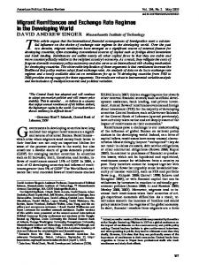
Setting numeric values for the ideological position of the two ministers at -2 and 2 for Finance and Minister, respectively and zero for the status quo, and varying the costs of losing office as well as varying am and a f , we predict Finance’s equilibrium proposal. Table 1 presents the results from the simulation6.
6
Placing the two ministers on either side of the status quo allows us to test for the
most interesting variation of the game, where the two ministers have opposing policy preferences and thus the policy conflict is the highest. 6
Table 1A: Numeric simulations for predicting Finance’s policy proposal to Minister
If ϑ f = −2
Cost of losing office Cost of losing office for both
ϑm = 2
for both parties is zero,
parties is moderate,
cm = c f = 0
cm = c f = 1
No electoral pledge
b f = b*f = 0
b f = b*f = 2 − 5 < 0
am = 0
Finance proposes an Finance
x0 = 0
af = 0
proposes
an
policy, acceptable policy, which is
acceptable
which is the status quo: closer to Finance’s ideal point than to Minister’s.
no policy change Strong
electoral
pledge
b f = b*f = 2 −
2
>0
3
b f = b*f = 2 −
am = 2
Finance proposes an Finance
af = 2
acceptable which
is
5 >0 3 proposes
an
policy, acceptable policy, which is closer
to closer to Minister’s ideal
Minister’s ideal point point than to Finance’s. than to Finance’s. Strong
electoral
pledge by M’s party
b f = b*f = 2 −
2
>0
3
b f = b*f = 2 −
am = 2
Finance proposes an Finance
af = 0
acceptable which
is
5 >0 3 proposes
an
policy, acceptable policy, which is closer
to closer to Minister’s ideal
Minister’s ideal point point than to Finance’s. than to Finance’s. Strong
electoral
pledge by F’s party
am = 0 af = 2
b f = b*f = 0
b f = b*f = 2 − 5 < 0
Finance proposes an
Finance
acceptable
proposes
an
policy, acceptable policy, which is
which is the status quo: closer to Finance’s ideal no policy change
point than to Minister’s.
7
Table 1 identifies the conditions under which there is no change in the policy status quo, when there is policy change closer to Finance’s ideal point and when the change is closer to Minister’s ideal point. Assuming both parties have similarly moderate costs of losing office, parties’ electoral pledges play a crucial role in the direction of policy change. When Minister’s party has made a strong pledge, irrespective of Finance’s party pledge, the policy proposal is to the right of the status quo and closer to Minister’s ideal policy than to Finance’s ideal policy. In contrast, when Minister’s party has not made a pledge, and Finance’s has, then the policy proposal, which is accepted by Minister, is to the left of the status quo and closer to Finance’s ideal point. Finally, when neither party has made a pledge, Finance proposes his ideal policy, which is not accepted by Minister, which leads to a policy dispute. Unlike the previous results, which are somewhat expected, the result that policy dispute is more likely when neither party has made a pledge and both parties are moderately office seeking is counter-intuitive. Finally, if we assume that neither party values office, or that there is no cost for having a policy dispute- which is possible-, we see two major outcomes: either there is no policy change, when the party of Minister has made no pledge, or Finance proposes a favorable to the Minister policy proposal, when Minister’s party has made a strong policy pledge, and irrespective of Finance’s party pledge. To sum up, the bargaining model provides the conditions for policy stability and policy change: policy stability is more likely in the absence of electoral pledges and when parties do not value office or when dispute is costless. Policy change is more likely when at least one of the parties has made a strong electoral pledge, and parties are moderately office-seeking or when there is a cost for having a policy dispute.
8
Section B Predicting the electoral benefits and costs of social democrats when controlling Social Affairs Here we seek to demonstrate that Social Democratic voters are attentive of both the promises and policies Social Democrats enact, while being in charge of the portfolio of Social Affairs. Adams (2012) notes that empirical evidence for the population noticing and punishing is scarce, but that it seems that both spatial modelers, in their assumptions, and party elites, in their actions, “believe that rankand-file voters do perceive and react to parties’ policy shifts”(p. 405). While not settled, retrospective economic voting is well established as a determinant of vote choice (see Lewis-Beck and Stegmaier (2015) for a review). To test whether these audience costs actually exist empirically, whether voters punish parties who fail to deliver on promises, we combined our data with data from the Comparative Study of Electoral Systems. We predict the individual level vote choice for 17 elections following a government. 7 In addition to several demographic and other relevant questions, the surveys ask how the voter voted in the most recent election, and how they did in the past election for 14 of the 17 cases. These data were combined with our data regarding the government that had occupied office before the election. Our argument suggests that voters should punish Social Democrats when they make a large pledge, welfare generosity decreases, and they hold the social affairs portfolio.
7
These election/countries are Austria in 2008; Belgium in 1999; Denmark in 1998,
2001, and 2007; Germany in 1998, 2002, 2005, and 2009; Ireland in 2002 and 2007, the Netherlands in 1998, 2006, and 2010; Norway in 2005 and 2009; and Portugal in 2005 9
Table 2A: Electoral costs for Social Democrats if they fail to uphold their welfare commitments
Delta Welfare Left Pledge Left in Government Left S. Affairs Welfare*Pledge Welfare*Left Gov. Ledge*Left Gov Welfare*Pledge*Left Gov Pledge*Left S. Affairs Welfare*Left S. Affairs Welfare*Pledge*Left SA Age Gender Education Household income Left/Right Unemployed Union member in HH Election Year Constant Observations t statistics in parentheses ="* p