analyze the incoming data in an online manner, tolerating but a constant time ... There are numerous applications for this type of data analysis such as, e.g., ...
Online Clustering of Data Streams J. Beringer and E. H¨ullermeier Informatics Institute, Marburg University, Germany {beringer,eyke}@mathematik.uni-marburg.de Abstract We consider the problem of clustering data streams. A data stream can roughly be thought of as a transient, continuously increasing sequence of time-stamped data. In order to maintain an up-to-date clustering structure, it is necessary to analyze the incoming data in an online manner, tolerating but a constant time delay. For this purpose, we develop an efficient online version of the classical K-means method. Our algorithm’s efficiency is mainly due to a (discrete) Fourier transform of the original data, resulting both in a smoothing as well as a compression of these data.
1 Introduction During the recent years, so-called data streams have attracted considerable attention in different fields of computer science, such as e.g. databases or distributed systems. As the notion suggests, a data stream can roughly be thought of as an ordered sequence of data items, where the input arrives more or less continuously as time progresses. There are various applications in which streams of this type are produced, such as e.g. network monitoring, telecommunication systems, customer click streams, stock markets, or any type of multi-sensor system. A data stream system may constantly produce huge amounts of data. To illustrate, imagine a multi-sensor system with 10,000 sensors, each of which sends a measurement every second of time. As concerns aspects of data storage, management and processing, the continuous arrival of data items in multiple, rapid, time-varying and potentially unbounded streams raises new challenges and research problems. Indeed, it is usually not feasible to simply store the arriving data in a traditional database management system in order to perform operations on that data later on. Rather, stream data must generally be processed in an online manner in order to guarantee that results are up-to-date and that queries can be answered with a small time delay. In this paper, we consider the problem of clustering data streams. Thus, our goal is to maintain classes of data streams such that streams within one class are similar to each other in a specific sense. Our focus is on time-series data streams, which means that individual data items are real numbers that can be thought of as a kind of measurement. There are numerous applications for this type of data analysis such as, e.g., clustering of stock rates. 1
Apart from its practical relevance, this problem is also interesting from a methodological point of view. Especially, the aspect of efficiency plays an important role: First, data streams are complex objects making the computation of similarity measures costly. Second, clustering algorithms for data streams should be adaptive in the sense that up-to-date clusters are offered at any time, taking new data items into consideration as soon as they arrive. The remainder of the paper is organized as follows: Section 2 provides some background information, both on data streams and on clustering. Section 3 is given to the clustering of data streams and introduces an online version of the well-known K-means algorithm. Some implementation issues are discussed in Section 4.
2 Background 2.1 The Data Stream Model The data stream model assumes that input data are not available for random access from disk or memory, but rather arrive in the form of one or more continuous data streams. The stream model differs from the standard relational model in the following ways [1]: • The elements of a stream arrive online (the stream is “active” in the sense that the incoming items trigger operations on the data, rather than being send on request). • The order in which elements of a stream arrive are not under the control of the system. • Data streams are potentially of unbounded size. • Data stream elements that have been processed are either discarded or archived. They cannot be retrieved easily unless being stored in memory, which is typically small relative to the size of the stream. (Stored information about past data is often referred to as a synopsis, see Fig. 1). • Due to limited resources (memory) and strict time constraints, the processing of stream data will usually produce approximate results.
2.2 Clustering Clustering refers to the process of grouping a collection of objects into classes or “clusters” such that objects within the same class are similar in a certain sense, and objects from different classes are dissimilar. In addition, the goal is sometimes to arrange the clusters into a natural hierarchy. Also, cluster analysis can be used as a form of descriptive statistics, showing whether or not the data consists of a set of distinct subgroups. Clustering algorithms proceed from given information about the similarity between objects, e.g. in the form of a proximity matrix. Usually, objects are described in terms of a set of measurements from which similarity degrees between pairs of objects are derived, using a kind of similarity or distance measure. There are basically three types 2
Synopsis in Memory 6 ?
Data Streams
- Stream Processing Engine -
- Approximate Answer
Figure 1: Basic structure of a data stream model.
of clustering algorithms: Mixture modeling assumes an underlying probabilistic model, namely that the data were generated by a probability density function, which is a mixture of component density functions. Combinatorial algorithms do not assume such a model. Instead, they proceed from an objective function to be maximized and approach the problem of clustering as one of combinatorial optimization. So called mode-seekers are somewhat similar to mixture models. However, they take a non-parametric perspective and try to estimate modes of the component density functions directly. Clusters are then formed by looking at the closeness of the objects to these modes which serve as cluster centers. One of the most popular clustering methods, the so-called K-means algorithm, belongs to the latter class. This algorithm starts by guessing K cluster centers and then iterates the following steps until convergence is achieved: • clusters are built by assigning each element to the closest cluster center; • each cluster center is replaced by the mean of the elements belonging to that cluster. K-means usually assumes that objects are described in terms of quantitative attributes, i.e. that an object is a vector x ∈ R n . Dissimilarity between objects is defined by the Euclidean distance, and the above procedure actually implements an iterative descent method that seeks to minimize the variance measure (“within cluster” point scatter) K �
�
|xı − x |2 ,
(1)
k=1 xı ,x ∈Ck
where Ck is the k-th cluster. In each iteration, the criterion (1) is indeed improved, which means that convergence is assured. Still, the final result may represent a suboptimal local minimum of (1) rather than a global optimum.
2.3 Related Work Several adaptations of standard statistical and data analysis methods to data streams or related models have been developed recently (e.g. [3, 11]). Likewise, several online 3
data mining methods have been proposed (e.g. [4, 8]). Clustering in connection with data streams has also been considered in [5] and [9]. In these works, however, the problem is to cluster the elements of one single data stream, which is clearly different from our problem, where the objects to be clustered are complete streams rather than single data items.
3 Clustering Data Streams The first question in connection with the clustering of (active) data streams concerns the concept of distance or, alternatively, similarity between streams. What does it mean that two streams are similar to each other and, hence, should fall into one cluster? Here, we are first of all interested in the time-dependent evolution of a data stream. That is to say, two streams are considered similar if their evolution over time shows similar characteristics. As an example consider two stocks both of which continuously increased between 9:00 AM and 10:30 AM but then started to decrease until 11:30 AM. To capture this type of similarity, we shall simply derive the Euclidean distance between the normalization of two streams (a more precise definition follows below) resp. the correlation between these streams. 1 Of course, there might be other reasonable measures of similarity for data streams or, more generally, time series [6], though Euclidean distance is commonly used in applications.
3.1 Data Streams and Sliding Windows The above example already suggests that one will usually not be interested in the entire data streams which are potentially of infinite length. At least, it is reasonable to assume that recent observations are more important than past data. Therefore, one often concentrates on a time window, that is a subsequence of a complete data stream. The most common type of window is a so-called sliding window which is of fixed length and comprises the w most recent observations. A more general approach to taking the relevancy of observations into account is that of weighing. Here, the idea is to associate a weight in the form of a real number to each observation such that more recent observations receive higher weights. Considering data streams in a sliding window of length w, a stream can formally be written as a w-dimensional vector X = (x 0 , x1 , . . . , xw−1 ), where a single observation xı is simply a real number. Due to reasons of efficiency, and since a single observation changes a stream but slightly, we further partition a window into m blocks (basic windows) of size v, hence w = m · v (Table 1 provides a summary of notation): X = ( x0 , x1 , . . . , xv−1 | xv , xv+1 , . . . , x2v−1 | . . . | x(m−1)v , x(m−1)v+1 , . . . , xw ) � �� � � �� � � �� � B1
B2
Bm
Data streams will then be updated in a “block-wise” manner each time v new items have been observed. We assume data items to arrive synchronously, which means that all 1 The correlation between normalized time series (with mean 0 and variance 1) is a linear function of their (squared) Euclidean distance.
4
symbol X Xn xı xı w m v c V x ¯ s
meaning data stream normalized data stream single observation ( + 1)-th element of block B ı window length length of a block number of blocks in a window weighing constant weight vector mean value of a stream standard deviation of a stream Table 1: Notation
streams will be updated simultaneously. An update of the stream X, in this connection also referred to as X old , is then accomplished by the following shift operation: X old : X
new
:
B1
| B2 | B3 | . . . | Bm−1 | Bm B2 | B3 | . . . | Bm−1 | Bm
| Bm+1
(2)
where Bm+1 denotes the entering block. We also consider an exponential weighing of observations, the weight attached to observation xı being defined by c w−ı−1 , where 0 < c ≤ 1 is a constant. V denotes the weight vector (c w−1 , . . . , c0 ), and V · X is the coordinate-wise product of V and a stream X, i.e. the sequence of values (c w−1 x0 , . . . , c0 xw ).
3.2 Normalization Since we are interested in the relative behavior of a data stream, the original streams are normalized in a first step. By normalization one usually means a linear transformation of the original data such that the transformed data has mean 0 and standard deviation 1. The corresponding transformation simply consists of subtracting the original mean and dividing the result by the standard deviation. Thus, we replace each value x ı of a stream X by its normalization xnı =def
5
xı − x ¯ . s
(3)
Considering the weighing of data streams, x ¯ and s are the weighted average and standard deviation, respectively: w−1 1−c � · xı · cw−ı−1 , 1 − cw ı=0
x ¯=
w−1 1−c � · (xı − x¯)2 · cw−ı−1 1 − cw ı=0
s2 =
w−1 1−c � = · (xı )2 · cw−ı−1 − (¯ x)2 . 1 − cw ı=0
As suggested above, x ¯ and s 2 are updated in a block-wise manner. Let X be a stream, and denote by x ı the ( + 1)-th element of the ı-th block B ı . Particularly, the exiting block leaving the current window (“to the left”) is given by the first block B 1 = (x10 , x11 , . . . , x1,v−1 ). Moreover, the new block entering the window (“from the right”) is Bm+1 = (xm+1,0 , xm+1,1 , . . . , xm+1,v−1 ). We maintain the following quantities for the stream X: q1 =def
w−1 �
xı · cw−ı−1 ,
q2 =def
ı=0
w−1 �
(xı )2 · cw−ı−1 .
ı=0
Likewise, we maintain for each block B k the variables qk1 =def
v−1 �
xkı · cv−ı−1 ,
qk2 =def
ı=0
v−1 �
(xkı )2 · cv−ı−1 .
ı=0
An update via shifting the current window by one block is then accomplished by setting q1 ← q1 · cv − q11 · cw + qm+1,1 , q2 ← q2 · cv − q12 · cw + qm+1,2 .
3.3 Discrete Fourier Transform The Discrete Fourier Transform (DFT) of a sequence X = (x 0 , . . . , xw−1 ) is defined through the DFT coefficients � � w−1 −i2πf 1 � x · exp DFTf (X) =def √ , f = 0, 1, . . . , w − 1 w w =0
√ where i = −1 is the imaginary unit. Denote by X n the normalized stream X defined through values (3). Moreover, denote by V the weight vector (c w−1 , . . . , c0 ) and recall that V · X n is the coordinatewise product of V and X n , i.e. the sequence of values cw−ı−1 · 6
¯ xı − x . s
Since the DFT is a linear transformation, which means that DFT(αX + βY ) = α DFT(X) + β DFT(Y ) for all α, β ≥ 0 and sequences X, Y , the DFT of V · X n is given by � � X−x ¯ DFT(V · X n ) = DFT V · s � � V · X − V · x¯ = DFT s =
DFT(V · X) − DFT(V ) · x ¯ . s
As can be seen, an incremental derivation is only necessary for DFT(V · X) while DFT(V ) can be computed in a preprocessing step.
3.4 Computation of DFT Coefficients Recall that the exiting and entering blocks are B 1 = (x10 , x11 , . . . , x1,v−1 ) and Bm+1 = (xm+1,0 , xm+1,1 , . . . , xm+1,v−1 ), respectively. Denote by X old = B1 |B2 | . . . |Bm the current and by X new = B2 |B3 | . . . |Bm+1 the new data stream. Without taking weights into account, the DFT coefficients are updated as follows [11]: DFTf (X new ) = e
i2πf v w
· DFTf (X old ) �v−1 v−1 � i2πf (v−) � i2πf (v−) 1 w w +√ e xm+1, − e x1, . w =0 =0
In connection with our weighing scheme, the weight of each element of the stream must be adapted as well. More specifically, the weight of each element x ı of X old is multiplied by cv , and the weights of the new elements x m+1, , coming from block B m+1 , are given by c v−−1 , 0 ≤ ≤ v − 1. Noting that DFT f (cv · X old ) = cv DFTf (X old ) due to the linearity of the DFT, the DFT coefficients are now modified as follows: DFTf (V · X new ) = e
i2πf v w
· cv DFTf (V · X old ) �v−1 v−1 � i2πf (v−) � i2πf (v−) 1 v−−1 w+v−−1 w w e c xm+1, − e c x1, . +√ w =0 =0
Using the values f βm+1 =def
v−1 �
e
i2πf (v−) w
cv−−1 xm+1, ,
=0
the above update rule simply becomes DFTf (V · X new ) = e
i2πf v w
� 1 f βm+1 − cw β1f . · cv DFTf (V · X old ) + √ w 7
(4)
1.5 1 0.5 0 −0.5 −1 0
50
100
150
200
250
300
350
400
Figure 2: Original (noisy) signal and DFT-filtered curve, using 40 out of 512 coefficients.
3.5 Distance Approximation and Smoothing We now turn to the problem of computing the Euclidean distance �w−1 1/2 � 2 |X − Y | = (xı − yı ) ı=0
between two streams X and Y in an efficient way. A useful property of the DFT is the fact that it preserves Euclidean distance, i.e. |X − Y | = | DFT(X) − DFT(Y ) | .
(5)
Furthermore, the most important information is contained in the first DFT coefficients. In fact, using only these coefficients within the inverse transformation (which recovers the original signal X from its transform DFT(X)) comes down to implementing a low-pass filter and, hence, to using DFT as a smoothing technique (see Fig. 2 for an illustration). Therefore, a reasonable idea is to approximate the distance (5) by using only the first u � w rather than all of the DFT coefficients and, hence, to store the values (4) only for f = 0, . . . , u − 1. More specifically, since the middle DFT coefficients are usually close to 0, the value 2
1/2
u−1 �
(DFTf (X) − DFTf (Y ))(DFTf (X) − DFTf (Y ))
f =1
is a good approximation to (5). Here, we have used that DFT w−f +1 = DFTf , where DFTf is the complex conjugate of DFT f . Moreover, the first coefficient DFT 0 can be dropped, as for real-valued sequences the first DFT coefficient is given by the mean of that sequence, which vanishes in our case (recall that we normalize streams in a first step). The above approximation has two advantages. First, by filtering noise we capture only the important properties of a stream. Second, the computation of the distance between two streams becomes much more efficient. 8
3.6 Clustering What we have got so far is an efficient method for incrementally computing the pairwise distance between data streams. Given this distance information, it is principally possible to apply any clustering method. Here, we propose an incremental version of the K-means algorithm. This algorithm appears especially suitable and can be extended in a natural way because it is already an iterative procedure. Our incremental K-means method works as follows: The standard K-means algorithm is run on the current data streams. As soon as a new block is available for all streams, the current streams are updated by the shift operation (2). Standard K-means is then simply continued. In other words, the clustering of the expired streams is taken as an initial solution for the clustering of the new streams. This solution will usually be good or even optimal since new streams will differ from the expired ones but slightly. An important additional feature that distinguishes our algorithm from standard Kmeans is an incremental adaptation of the cluster number K. Needless to say, such an adaptation is very important in the context of our application where the clustering structure can change over time. Choosing the right number K is a question of practical importance also in standard K-means, and a number of (heuristic) strategies have been proposed. A common approach is to look at the cluster dissimilarity (the sum of distances between objects and their associated cluster centers) for a set of candidate values K ∈ {1, 2, . . . , Kmax }. The cluster dissimilarity is a decreasing function of K, and one expects that this function will show a kind of irregularity at K ∗ , the optimal number of clusters. This intuition has been formalized, e.g., by the recently proposed gap statistic [10]. Unfortunately, the above strategy is not practicable in our case, as it requires the consideration of too large a number of candidate values. Our adaptation process rather works as follows: In each iteration phase, one test is made in order to check whether the clustering structure can be improved by increasing or decreasing K ∗ , the currently optimal cluster number. By iteration phase we here mean the phase between the entry of new blocks, i.e. while the streams to be clustered remain unchanged. We restrict ourselves to adaptations of K ∗ by ±1, which is again justified by the fact that the clustering structure will usually not change abruptly. We make use of a quality measure in order to evaluate a clustering structure. Roughly speaking, this measure adds to the cluster dissimilarity a penalty term λ · K that punishes large values K. The scaling factor λ puts the penalty into a reasonable relation to the cluster dissimilarity which depends on the absolute distances between the objects to be clustered. We found that the mean distance between all cluster centers is a good choice for λ. This value is derived from the current clustering in each iteration phase. Let Q(K) denote the above quality measure for the cluster number K resp. the clustering obtained for this number. The optimal cluster number is then updated as follows: K ∗ ← arg max{Q(K ∗ − 1), Q(K ∗ ), Q(K ∗ + 1)}. Intuitively, going from K ∗ to K ∗ − 1 means that one cluster has disappeared. Thus, Q(K ∗ − 1) is derived from the best clustering that can be obtained by removing one
9
Figure 3: First online visualization tool.
of the current clusters re-assigning each element of the removed cluster to the closest cluster among the remaining ones. Going from K ∗ to K ∗ +1 assumes that an additional cluster has emerged. To create this cluster we complement the existing K ∗ centers by one center which is defined by a randomly chosen object (stream). The probability of a stream to be selected is reasonably defined as an increasing function of the stream’s distance from its cluster center. In order to compute Q(K ∗ + 1) we try out a fixed number of randomly chosen objects and select the one which gives the best clustering.
4 Implementation Our online clustering method has been implemented under XXL (eXtensible and fleXible Library). The latter is a JAVA library for query processing developed and maintained at the Informatics Institute of Marburg University [2], and meanwhile utilized by numerous (international) research groups. Apart from several index structures, this library offers built-in operators for creating, combining and processing queries. As the name suggests, the basic philosophy of XXL is its flexibility and the possibility to easily extend the library. Currently, a package called PIPES is developed for the handling of active data streams. This package offers abstract classes for the implementation of data sources and operators, which can be combined into so-called query graphs in a flexible way. We have used PIPES for our implementation. Roughly speaking, the process of clustering corresponds to an operator. As inputs this operator receives (blocks of) data items from the (active) data streams. As outputs it produces the current cluster number for each stream. This output can be used by any other operator, e.g. by visualization tools that we have developed as well. Fig. 3 shows an example of an online visualization. Basically, this tool shows a table whose rows correspond to the data streams. What can be seen here is the top of a list consisting of 230 stock rates whose overall length is 230. Each column stands for one cluster, and a stream’s current cluster is indicated by a square. Thus, a square moves horizontally each time the clustering structure changes, making this tool very 10
Figure 4: Second online visualization tool.
convenient for visual inspection. Further, each cluster is characterized by means of a prototypical stream showing the qualitative behavior of the streams in that cluster. As can be seen, in our example there are currently three types of stock rates showing a similar evolution over the last 16 hours, the size of the sliding window. The first type, for instance, decreased slightly during the first half of that time period and then began to increase until so far. A second visualization tool, illustrated in Fig. 4, shows the recent history of the clustering structure, rather than only the current state. Again, each row corresponds to a stream. Now, however, each column corresponds to a time point. Each cluster is identified by a color (here a symbol for better visualization), and these colours are used to identify a stream’s cluster at the different time points.
5 Concluding Remarks We have introduced an online version of the K-means algorithm for clustering data streams. A key aspect of our method is an efficient incremental computation of the distance between such streams, using a DFT approximation of the original data. This way, it becomes possible to cluster several thousands of data streams in real-time. In order to investigate the performance of our approach we are currently performing several controlled experiments with synthetic data. 2 Especially, these experiments are meant to throw light on the scalability of the method and on the tradeoff between runtime complexity and quality of the clustering. All in all, our first results show that the method achieves an extreme gain in complexity at the cost of an acceptable (often very small) loss in quality. (In case of acceptance, the results will be incorporated in the final version of the paper.) We are also extending our method in several directions. Inter alia, we are implementing a fuzzy version of K-means [7]. In fuzzy cluster analysis, an object can belong to more than one cluster, and the degree of membership in each cluster in characterized by means of a number between 0 and 1. This extension of the standard approach appears particularly reasonable in the context of online clustering: If a data stream moves from one cluster to an other cluster, it usually does so in a “smooth” rather than an abrupt manner. 2 Currently,
real-world data is very difficult to obtain for this type of application.
11
References [1] Brian Babcock, Shivnath Babu, Mayur Datar, Rajeev Motwani, and Jennifer Widom. Models and issues in data stream systems. In Proceedings of the Twentyfirst ACM SIGACT-SIGMOD-SIGART Symposium on Principles of Database Systems, June 3-5, Madison, Wisconsin, USA, pages 1–16. ACM, 2002. [2] J. Bercken, B. Blohsfeld, J. Dittrich, J. Kr¨amer, T. Sch¨afer, M. Schneider, and B. Seeger. XXL - A library approach to supporting efficient implementations of advanced database queries. In Proc. of the VLDB, pages 39–48, 2001. [3] M. Datar, A. Gionis, P. Indyk, and R. Motwani. Maintaining stream statistics over sliding windows. In Proc. of the Annual ACM-SIAM Symp. on Discrete Algorithms (SODA 2002), 2002. [4] Mayur Datar and S.Muthukrishnan. Estimating rarity and similarity over data stream windows. In Algorithms - ESA 2002, pages 323–334. Springer, 2002. [5] Sudipto Guha, Nina Mishra, Rajeev Motwani, and Liadan O’Callaghan. Clustering data streams. In IEEE Symposium on Foundations of Computer Science, pages 359–366, 2000. [6] D. Gunopulos and G. Das. Time series similarity measures and time series indexing. In Proc. 2001 ACM SIGMOD International Conference on Management of Data, Santa Barbara, California, 2001. [7] F. H¨oppner, F. Klawonn, R. Kruse, and T. Runkler. Fuzzy Cluster Analysis: Methods For Classification, Data Analysis and Image Recognition. Wiley, 1999. [8] Geoff Hulten, Laurie Spencer, and Pedro Domingos. Mining time-changing data streams. In Proceedings of the seventh ACM SIGKDD international conference on Knowledge discovery and data mining, pages 97–106. ACM Press, 2001. [9] L. O’Callaghan, N. Mishra, A. Meyerson, S. Guha, and R. Motwani. Streamingdata algorithms for high-quality clustering, 2002. [10] R. Tibshirami, G. Walther, and T. Hastie. Estimating the number of clusters in a data set via the gap statistic. Journal of the Royal Statistical Society – Series B, 63(2):411–423, 2001. [11] Y. Zhu and D. Shasha. Statstream: Statistical monitoring of thousands of data streams in real time, 2002.
12