Online Constrained Receding Horizon Control for ...

Online Constrained Receding Horizon Control for Astronomical Adaptive Optics by

Mikhail Konnik

Thesis submitted in partial fullment of the requirements for the Degree of

Doctor of Philosophy

School of Electrical Engineering and Computer Science

August, 2013

c Copyright

by

Mikhail Konnik 2013

Online Constrained Receding Horizon Control for Astronomical Adaptive Optics

Statement of Originality This work contains no material which has been accepted for the award of any other degree or diploma in any university or other tertiary institution and, to the best of my knowledge and belief, contains no material previously published or written by another person, except where due reference has been made in the text. I give consent to this copy of my thesis, when deposited in the University Library, being made available for loan and photocopying subject to the provisions of the Copyright Act 1968.

Mikhail Konnik 27th August 2013

iii

Acknowledgments Many people have helped, encouraged, and supported me during the research and writing of this thesis. My deepest appreciation goes to Prof. Jose De Dona, who supported and encouraged me throughout the most dicult part of my postgraduate study and research. His immense knowledge of control theory, enthusiasm and positive outlook have been a constant beacon of encouragement to pursue the sometimes dicult results. To Jose I express my most sincere and wholehearted gratitude. I would like to extend my gratitude to Dr. James Welsh for his invaluable help in the early stage of the project, and to Prof. Peter Schreier who opened up the world of advanced linear algebra for me. Many thanks to Dr. Rodolphe Conan for his hospitality during my visit to ANU RSAA, and to Prof. Mazen Alamir for a fruitful discussion that gave valuable hints for my research project. I am indebted to the faculty and general sta members of the School of Electrical and Computer Engineering for their help and support. Thanks to Kathy Allan, Kathryn Killen, Chanel Hopkinson and Sally Ann Heron who helped me with formal matters. Special thanks to Dianne Piefke and Jayne Disney for their ecient and cheerful assistance. My sincere appreciation goes to fellow postgraduate students with whom I have had the good fortune to share many experiences in Newcastle. Special thanks to Rahmat Heidari, Ali Mohammadee, Raheleh Nazari, Majid Hosseini, Kasun Thotahewa, and Saeid Mehrkanoon for the many fruitful discussions on research topics and beyond. All the best with your theses. Last but not the least, my warmest regards to Ansel and Solara Zwaneveld, who have turned Newcastle into my home. Solara's excellent cooking gave me all the energy to undertake such a challenging research, and Ansel's constant philosophical support kept me on track. And, of course, a huge thanks to my parents, Galina and Vsevolod Konnik, for their support and understanding thousands miles away from the home.

Mikhail Konnik

The University of Newcastle August 2013

iv

Table of Contents Page Acknowledgments . . . . . . . . . . . . . . . . . . . . . . . . . . . . . . . . . . .

iv

Abstract . . . . . . . . . . . . . . . . . . . . . . . . . . . . . . . . . . . . . . . . .

ix

Publications and Outcomes . . . . . . . . . . . . . . . . . . . . . . . . . . . . .

x

Acronyms and Abbreviations . . . . . . . . . . . . . . . . . . . . . . . . . . . . xiii 1 Introduction . . . . . . . . . . . . . . . . . . . . . . . . . . . . . . . . . . . .

1

1.1

Optimal and Classical control in Adaptive Optics . . . . . . . . . . . . . . .

2

1.2

Contributions of this Thesis . . . . . . . . . . . . . . . . . . . . . . . . . . .

4

1.3

Thesis Overview . . . . . . . . . . . . . . . . . . . . . . . . . . . . . . . . .

6

2 Where optics meets automatic control: Adaptive Optics . . . . . . . . . 2.1

2.2

2.3

2.4

2.5

9

Adaptive Optics for Astronomy . . . . . . . . . . . . . . . . . . . . . . . . . 10 2.1.1

Wavefront Sensing . . . . . . . . . . . . . . . . . . . . . . . . . . . . 12

2.1.2

Wavefront Reconstruction . . . . . . . . . . . . . . . . . . . . . . . . 14

Deformable Mirrors and Actuators . . . . . . . . . . . . . . . . . . . . . . . 16 2.2.1

Actuators for Deformable Mirrors . . . . . . . . . . . . . . . . . . . . 17

2.2.2

Types of Deformable Mirrors . . . . . . . . . . . . . . . . . . . . . . 18

2.2.3

Current technologies for Deformable Mirrors . . . . . . . . . . . . . . 18

2.2.4

Desirable parameters of Deformable Mirrors . . . . . . . . . . . . . . 22

Control Strategies for Adaptive Optics Systems . . . . . . . . . . . . . . . . 23 2.3.1

Control techniques currently used in Adaptive Optics . . . . . . . . . 23

2.3.2

Proposed control strategy: constrained Receding Horizon Control . . 23

2.3.3

Alternative Solutions and Approaches for Constrained Control

2.3.4

Receding Horizon Control for Adaptive Optics . . . . . . . . . . . . . 24

. . . 24

Optimisation Strategies for Receding Horizon Control in Adaptive Optics . 25 2.4.1

Quadratic and Linear Programming . . . . . . . . . . . . . . . . . . 25

2.4.2

Optimal Control Problem Formulation: Linear or Quadratic? . . . . 26

2.4.3

Which optimisation formulation is preferable for Adaptive Optics? . 28

Chapter Summary . . . . . . . . . . . . . . . . . . . . . . . . . . . . . . . . 28

3 Optimal control for Adaptive Optics: from Innite to Receding Horizon 29 3.1

Dynamic models of Adaptive Optics components . . . . . . . . . . . . . . . 29 3.1.1

The model of a wavefront sensor . . . . . . . . . . . . . . . . . . . . 29

3.1.2

Dynamic Models of Deformable mirrors . . . . . . . . . . . . . . . . 30

3.1.3

Coupling models for actuators in Deformable Mirrors . . . . . . . . . 30 v

3.2

3.3

3.4

3.1.4

Typical sampling rate of an Adaptive Optics system . . . . . . . . . 33

3.1.5

Output disturbance dynamics . . . . . . . . . . . . . . . . . . . . . . 33

3.1.6

The complete model of an Adaptive Optics system . . . . . . . . . . 33

Formulation of Linear Quadratic Gaussian control for Adaptive Optics . . . 34 3.2.1

Linear Quadratic Gaussian control for Adaptive Optics . . . . . . . . 34

3.2.2

Formulation of Linear Quadratic Gaussian control . . . . . . . . . . 35

3.2.3

Numerical issues of the optimal control for Adaptive Optics systems

3.2.4

Summary for Linear Quadratic Regulator control . . . . . . . . . . . 37

35

From Innite to Receding Horizon control . . . . . . . . . . . . . . . . . . . 38 3.3.1

Motivation for constrained optimal control in Adaptive Optics . . . . 38

3.3.2

The main idea behind Receding Horizon Control . . . . . . . . . . . 39

3.3.3

Formulation of Receding Horizon Control for Adaptive Optics . . . . 40

Accounting for hard constraints: Constrained Receding Horizon Control . . 42 3.4.1

Motivational example: Wae mode mitigation in Adaptive Optics using the Constrained Control approach . . . . . . . . . . . . . . . . 43

3.5

3.4.2

Discussion of wae modes mitigation via constrained control . . . . 45

3.4.3

Summary for constrained Receding Horizon Control . . . . . . . . . 46

Initial assessment of applicability of Receding Horizon Control in Adaptive Optics using general-purpose Quadratic Programming algorithms . . . . . . 47 3.5.1

Results for the decoupled case . . . . . . . . . . . . . . . . . . . . . . 48

3.5.2

Results for the case of coupling between nearest neighbour actuators

3.5.3

Results for the case of coupling between nearest neighbour and di-

49

agonally adjacent actuators . . . . . . . . . . . . . . . . . . . . . . . 49

3.6

3.5.4

Discussion of simulations results . . . . . . . . . . . . . . . . . . . . 50

3.5.5

Summary of initial assessment of Receding Horizon Control . . . . . 51

Chapter Summary . . . . . . . . . . . . . . . . . . . . . . . . . . . . . . . . 52

4 Structure of the Hessian matrix in optimal control of Deformable Mirrors . . . . . . . . . . . . . . . . . . . . . . . . . . . . . . . . . . . . . . . . . . 55 4.1

Structure of the Hessian matrix in constrained optimal control for Adaptive Optics . . . . . . . . . . . . . . . . . . . . . . . . . . . . . . . . . . . . . . . 56

4.2

4.1.1

Considered cases of inter-actuators coupling . . . . . . . . . . . . . . 56

4.1.2

The length of a prediction horizon and the matrices structure . . . . 58

Inter-actuators coupling and its inuence on the matrices structure . . . . . 60 4.2.1

No coupling between actuators . . . . . . . . . . . . . . . . . . . . . 60

4.2.2

Coupling between four nearest neighbour actuators only . . . . . . . 61

4.2.3

Coupling between four nearest neighbours and four diagonally adjacent actuators . . . . . . . . . . . . . . . . . . . . . . . . . . . . . . . 61

4.3

4.4

Time-delays augmentation of Receding Horizon Control matrices . . . . . . 63 4.3.1

Sources of delays in Adaptive Optics . . . . . . . . . . . . . . . . . . 63

4.3.2

Augmentation of state space matrices for time delays . . . . . . . . . 63

Thresholding matrices in optimisation problem and sparsity patterns . . . . 65 4.4.1

Coupling between nearest neighbour actuators . . . . . . . . . . . . . 65 vi

4.4.2 4.5

Coupling between nearest and diagonally adjacent actuators . . . . . 66

Inter-actuators coupling and condition number of the Hessian matrix . . . . 68 4.5.1

Relationships between the condition number of the Hessian matrix and actuators properties . . . . . . . . . . . . . . . . . . . . . . . . . 68

4.5.2

Condition number and coupling: case of four nearest actuator coupling 69

4.5.3

Condition number and coupling: case of four nearest and four diagonally adjacent actuators coupling . . . . . . . . . . . . . . . . . . . 72

4.5.4

Results Discussion . . . . . . . . . . . . . . . . . . . . . . . . . . . . 73

4.6

Structure exploiting in optimisation problems . . . . . . . . . . . . . . . . . 74

4.7

Chapter Summary . . . . . . . . . . . . . . . . . . . . . . . . . . . . . . . . 76

5 Advanced Optimisation Algorithms for Adaptive Optics Control . . . 5.1

5.2

5.3

77

Choosing Algorithms for Constrained Convex Quadratic Optimisation . . . 77 5.1.1

Active Set QP methods . . . . . . . . . . . . . . . . . . . . . . . . . 78

5.1.2

Interior point QP methods . . . . . . . . . . . . . . . . . . . . . . . . 81

5.1.3

Branch and Bound QP methods

5.1.4

Gradient-based QP methods . . . . . . . . . . . . . . . . . . . . . . . 84

5.1.5

Summary of optimisation algorithms . . . . . . . . . . . . . . . . . . 85

. . . . . . . . . . . . . . . . . . . . 83

Gradient-based optimisation algorithms . . . . . . . . . . . . . . . . . . . . 87 5.2.1

Barzilai-Borwein optimisation algorithm . . . . . . . . . . . . . . . . 88

5.2.2

Gradient Projection algorithm . . . . . . . . . . . . . . . . . . . . . . 91

5.2.3

Conjugate Gradients methods for Quadratic Programming . . . . . . 92

5.2.4

Pre-Conditioned Conjugate Gradients . . . . . . . . . . . . . . . . . 93

5.2.5

Constrained Gradient Projection Conjugate Gradients . . . . . . . . 96

Active Set Quadratic Programming Algorithms . . . . . . . . . . . . . . . . 102 5.3.1

Primal Range-Space Active Set QP algorithm . . . . . . . . . . . . . 102

5.3.2

Dual Active Set QP algorithm . . . . . . . . . . . . . . . . . . . . . . 109

5.3.3

Parametric Active Set algorithm . . . . . . . . . . . . . . . . . . . . 111

5.4

Branch and Bound algorithm . . . . . . . . . . . . . . . . . . . . . . . . . . 112

5.5

Chapter Summary . . . . . . . . . . . . . . . . . . . . . . . . . . . . . . . . 114

6 Feasibility of Constrained Receding Horizon Control in Adaptive Optics115 6.1

Details of the Numerical Simulations . . . . . . . . . . . . . . . . . . . . . . 115

6.2

Preliminary assessment of Receding Horizon Control feasibility . . . . . . . 117 6.2.1

Computational feasibility of RHC: Primal-Dual Predictor-Corrector Interior Point QP algorithm . . . . . . . . . . . . . . . . . . . . . . . 118

6.3

6.2.2

Computational feasibility of RHC: Dual Active Set QP . . . . . . . . 120

6.2.3

Results discussion and further choice of QP algorithms . . . . . . . . 123

Feasibility of Receding Horizon Control for adaptive optics using customized optimisation algorithms . . . . . . . . . . . . . . . . . . . . . . . . . . . . . 123 6.3.1

Results for Branch and Bound QP algorithm . . . . . . . . . . . . . 124

6.3.2

Results for Range-Space Primal Active Set QP algorithm . . . . . . 127

6.3.3

Results for Parametric Active Set algorithm qpOASES . . . . . . . . 135 vii

6.3.4

Results for Barzilai-Borwein PABB QP algorithm . . . . . . . . . . . 138

6.3.5

Results for Gradient Projection Conjugate Gradients algorithm . . . 149

6.3.6

Results for Gradient Projection Preconditioned Conjugate Gradients algorithm . . . . . . . . . . . . . . . . . . . . . . . . . . . . . . . . . 156

6.4

Chapter Summary . . . . . . . . . . . . . . . . . . . . . . . . . . . . . . . . 164

7 Performance evaluation for Receding Horizon Control in Adaptive optics167 7.1

Saturation versus constrained optimisation: A Motivational Example . . . . 167 7.1.1

An illustrative example of constrained optimisation in the presence of coupling . . . . . . . . . . . . . . . . . . . . . . . . . . . . . . . . 169

7.2

7.1.2

The unconstrained case . . . . . . . . . . . . . . . . . . . . . . . . . 170

7.1.3

The constrained case . . . . . . . . . . . . . . . . . . . . . . . . . . . 170

7.1.4

Summary for the illustrative example . . . . . . . . . . . . . . . . . . 171

Initial comparison of the residual disturbance for Linear Quadratic Regulator and Receding Horizon Control . . . . . . . . . . . . . . . . . . . . . . . . 172 7.2.1

Details of Numerical Simulations for the comparison of LQR and RHC controllers performance . . . . . . . . . . . . . . . . . . . . . . 173

7.3

7.2.2

Performance comparison for the unconstrained case . . . . . . . . . . 173

7.2.3

Performance comparison for the constrained case . . . . . . . . . . . 174

7.2.4

Summary for initial comparison of disturbance rejection performance 176

Output disturbance rejection performance for Receding Horizon Control and Linear Quadratic Regulator . . . . . . . . . . . . . . . . . . . . . . . . . . . 176

7.4

7.3.1

High-gain control case . . . . . . . . . . . . . . . . . . . . . . . . . . 177

7.3.2

Low-gain control case . . . . . . . . . . . . . . . . . . . . . . . . . . 179

7.3.3

Optimised gain control case . . . . . . . . . . . . . . . . . . . . . . . 181

7.3.4

Summary of the disturbance rejection performance comparison . . . 182

Computational burden for Linear Quadratic Regulator and Receding Horizon Control . . . . . . . . . . . . . . . . . . . . . . . . . . . . . . . . . . . . 184 7.4.1

Computational time evaluation for Linear Quadratic Control . . . . 185

7.4.2

Comparison of computational burden for Receding and Innite Horizon Control . . . . . . . . . . . . . . . . . . . . . . . . . . . . . . . . 185

7.4.3 7.5

Summary of computational time comparison . . . . . . . . . . . . . . 189

Chapter Summary . . . . . . . . . . . . . . . . . . . . . . . . . . . . . . . . 189

8 Conclusions and Future work . . . . . . . . . . . . . . . . . . . . . . . . . . 191 8.1

Summary of the Results . . . . . . . . . . . . . . . . . . . . . . . . . . . . . 191 8.1.1

A summary of the main results . . . . . . . . . . . . . . . . . . . . . 192

8.1.2

The novel contributions . . . . . . . . . . . . . . . . . . . . . . . . . 194

8.2

Thesis Reection . . . . . . . . . . . . . . . . . . . . . . . . . . . . . . . . . 194

8.3

Future Research . . . . . . . . . . . . . . . . . . . . . . . . . . . . . . . . . . 195

Bibliography . . . . . . . . . . . . . . . . . . . . . . . . . . . . . . . . . . . . . . 197

viii

Abstract Actuators are naturally limited in the force they can apply, and eciency often dictates operation that is close to the limits of the permissible values. This is especially true for adaptive optics systems that compensate for the atmospheric turbulence using the mirrors deformable on-the-y by the actuators. On the one hand, the actuator should use all the authority to bend the deformable mirror and thus compensate the turbulence. On the other hand, the actuators must not damage the mirror by pushing the surface too hard, and the controller must account for these constraints. This thesis focuses on the high-speed constrained control of deformable mirrors in astronomical adaptive optics. The main approach considered in this work is constrained Receding Horizon Control with Quadratic Programming. A thorough study of the structure and the physics of the control problem allowed exploiting the structure of the problem and an inherently fast sampling rate to hot-start the online optimisation. These features are of crucial importance, making it possible to accelerate the constrained control by magnitude

orders of

compared to standard algorithms.

The original contribution of this thesis is a thorough feasibility analysis of the online optimisation algorithms for constrained control in adaptive optics systems. While the Convex Optimisation and the Receding Horizon Control are well studied areas, their application for astronomical adaptive optics has not been systematically studied. The thesis provides the results of numerical simulations that conclusively prove the feasibility of online constrained control of a deformable mirror. Using state-of-the-art Quadratic Optimisation algorithms of my own implementation, a control rate of 10 kHz for a relatively large deformable mirror has been achieved. The signicance of the results of this thesis is a comprehensive performance analysis of various optimisation approaches for constrained optimal control of deformable mirrors in adaptive optics. This is an important step towards attaining the ultimate compensation potential of adaptive optics systems.

ix

Publications and Outcomes The material presented in this Thesis has been already published, or accepted for publication, in peer-reviewed journals and conferences. Some of the material has been recently submitted for publication. The list of publications is provided below.

Articles in peer-reviewed journals Mikhail V. Konnik and James Welsh (2013, submitted), On high-level numerical simulations of noise in solid-state photosensors: a Review .

Journal on Simulations

Mikhail V. Konnik and Jose De Dona (2013, under review, TCST-2012-0662), Feasibility of Constrained Receding Horizon Control Implementation in Adaptive Optics .

IEEE Transactions on Control Systems Technology

Mikhail V. Konnik and James S. Welsh (2012), Performance of a discrete Linear Quadratic Gaussian controller with a realistic noise model for adaptive optics systems.

GSTF Journal on Computing,

vol.2, num.3, pages 76-85.

Conference proceedings Mikhail V. Konnik and Jose De Dona (2013), Wae mode mitigation in adaptive optics systems: a constrained Receding Horizon Control approach .

Proceedings of

American Control Conference (ACC), page 33963402, Washington, DC, USA

Mikhail Konnik, Jose De Dona and James Stuart Welsh (2012) Constrained control of low order adaptive optics systems using a fast suboptimal solution based on feedback from coupling, in Proceedings of Australian Control Conference (AuCC), Sydney, 15-16 November 2012. Pages 313-319

Mikhail V. Konnik and James Welsh (2012), Open-source framework for documentation of scientic software written on MATLAB-compatible programming languages, In

Proceedings of SPIE Astronomical Telescopes + Instrumentation - Software and

Cyberinfrastructure for Astronomy II,

8451-102, Amsterdam, The Netherlands.

Mikhail V. Konnik and Jose De Dona and James Stuart Welsh(2012), On application of constrained receding horizon control in astronomical adaptive optics, In Proceedings of SPIE Astronomical Telescopes + Instrumentation - Adaptive Optics Systems III,

8447-110. Amsterdam, The Netherlands. x

Mikhail V. Konnik (2012), Hybrid optical-digital encryption system based on wavefront coding paradigm, In

Proceedings of SPIE Defence, Security, and Sensing -

Optical Pattern Recognition XXIII,

8398-25. Baltimore, MD, USA.

Mikhail V. Konnik (2012), Using wavefront coding technique as an optical encryption system: reliability analysis and vulnerabilities assessment In

Proceedings of SPIE

Defence, Security, and Sensing - Optical Pattern Recognition XXIII.,

8398-27. Bal-

timore, MD, USA.

Mikhail V. Konnik and James S. Welsh (2012) The inuence of measurement noise on the performance of a discrete Linear Quadratic Gaussian controller for adaptive optics systems in

Proceedings of 2nd Annual International Conference on Control,

Automation and Robotics (CAR 2012),

Bangkok, Thailand, pages 17.

Mikhail V. Konnik and James Welsh (2011), Wavefront Noise Reduction in a ShackHartmann Wavefront Sensor using Kalman lter, In

International Symposium on

Optomechatronic Technologies (ISOT), November 1-3,,

pages 334339. Hong Kong.

Mikhail V. Konnik and James Welsh (2011), On numerical simulation of high-speed CCD/CMOS-based wavefront sensors in adaptive optics, In Proceedings tical Engineering + Applications,

of SPIE Op-

paper 8149-15. San Diego, CA, USA.

Mikhail V. Konnik and James Welsh (2011), Inuence of photosensor noise on ac-

S

H

curacy of cost-eective hack- artmann wavefront sensors, In Optical Engineering + Applications,

Proceedings of SPIE

paper 8149-16. San Diego, CA, USA.

Software development Research software for adaptive optics has been developed in MATLAB and ANSI C by the author as a part of this Ph.D. project.

Adaptive Optics Real Time Analyser (AORTA) All the numerical simulations in this project were carried out using my own MATLABbased simulator with C/MEX routines for speed-up. The AORTA simulator was written in the form of a toolbox of interconnected functions and was extensively documented using Doxygen. The code of the simulator contains about

65000 lines of MATLAB code

and

about 6000 lines of documentation. The following features have been implemented:

3

Atmosphere

and phase screens are generated using the Taylor frozen-turbulence hy-

pothesis, Models of power spectrum of atmosphere turbulence (Kolmogorov, Tatarskii, von Karman, Modied von Karman, Hill), Hufnagel-Valley, Mauna Kea),

models of turbulence

optical propagators

(pure Hufnagel,

(Fresnel, Fraunhofer, Angular

spectrum propagation);

3

Photosensor model

with light noise (photo response non-uniformity, photon shot

noise), dark noise (dark current shot noise, dark current xed pattern noise, source xi

follower noise, sense node reset noise (kTC noise), oset xed pattern noise) and ADC (quantisation noise);

3

Laser guide star

3

Wavefront sensor :

(Rayleigh scattering, sodium beacons, NGS); Shack-Hartmann, with variable lenslets size/amount and photo-

sensor model, centroiding algorithms (CoG, WCoG);

3

Wavefront reconstructors :

Fried (FFT-based), Hudgin (classical and modied, via

FFT), Southwell, Least-squares, Zernike modes;

3

Deformable Mirrors :

3

Control :

DM with inuence functions and Thin Plate Splines;

Discrete PI, discrete LQG, discrete MPC.

Quadratic Programming Faster-Than-Light (QPFTL) QPFTL is the toolbox for the convex quadratic optimisation of my own implementation. The algorithms are customised specically to exploit the structure and physics of the Adaptive Optics problem. The QP solvers are written in MATLAB and ANSI C with the BLAS routines and compiled as MEX les. The qpOASES algorithm (one of the fastest available) has been outperformed by my

own QPFTL solver

in AO problems. The following

QP solvers were implemented:

3 Primal-Dual Interior Point (Predictor-Corrector, Directed Cones); 3 Primal and Dual Active Set (Range-space and Null-space); 3 Gradient-based (GPCG, PABB, SPG, PSPG, Projection-Contraction); 3 Branch-and-Bound (breed-rst, depth-rst); 3 and other methods (Hildreth-D'Ezopo, Jacobi iterations, Dantzig-Wolfe). Various pre-conditioner strategies (Jacobi, SSOR, incomplete Cholesky) were implemented, along with structure exploiting methods. QPFTL takes advantage of the custom implementation of QPs, gains signicant acceleration in terms of computational time (typically 50-100x compared to MATLAB code), and is able to be called directly from MATLAB. The AORTA simulator uses QP routines from QPFTL to estimate the computational time of the optimisation algorithms.

xii

Acronyms and Abbreviations Acronym...

stands for

AS

Active Set (type of optimisation algorithms)

AO

Adaptive Optics

AS WGS BaB BLAS CCD CG

Active Set with Weighting Gram-Schmidt Branch-and-Bound (type of the optimisation algorithms) Basic Linear Algebra Subroutine Charge Coupled Device (photosensor type) Conjugate Gradients (optimisation algorithm)

CMOS

Complimentary Metal Oxide Semiconductor (photosensor type)

DARE

Discrete Algebraic Riccati Equation

DM FFT GP GPCG GPpreconCG IP KKT LAPACK

Deformable Mirror Fast Fourier Transform Gradient Projection Gradient Projection Conjugate Gradients Gradient Projection Preconditioned Conjugate Gradients Interior Point (type of optimisation algorithms) Karush-Kuhn-Tucker (optimality conditions) Linear Algebra Package

LP

Linear Programming

LQ

lower triangular (L) - orthogonal (Q) matrix decomposition

LQG

Linear Quadratic Gaussian (type of control)

LQR

Linear Quadratic Regulator (type of control)

MPC

Model Predictive Control

OS PABB

Operating System Projected Alternating Barzilai-Borwein

PI

Proportional-Integration (type of control)

PI

Proportional-Integration-Derivative (type of control)

QP

Quadratic Programming

QR

orthogonal (Q) - triangular (R) matrix decomposition

RHC RSPAS RTOS

Receding Horizon Control (type of control) Range-Space Primal Active Set (same as AS WGS) Real Time Operating System

SH

Shack-Hartmann (wavefront sensor)

TF

Transfer Function

TM

Transfer Matrix

WFR

Wavefront reconstruction

WFS

Wavefront sensor

xiii

xiv

Chapter 1

Introduction - The word impossible is not in my dictionary.

T

Napoleon Bonaparte

urbulence of the Earth's atmosphere produces inhomogeneity in the air refractive index that diers for hot and cold air. The volume distribution of the refractive index can be thought of as a surface, or a wavefront. If there is no

atmospheric turbulence, the wavefront will be at, which means that all the light rays have travelled the same distance. Due to mixing of hot and cold air along with strong wind gusts, the wavefront becomes non-at, which causes the light to travel dierently. In turn, this causes blurring of astronomical images acquired by ground-based telescopes. Adaptive Optics (AO) systems use a reference wavefront to estimate the aberration induced by the atmospheric turbulence and compensate for the wavefront error. The distortions caused by the atmosphere are estimated by a wavefront sensor (WFS). To compensate for the atmospheric turbulence, the shape of the deformable mirror (DM) is adjusted in real-time by actuators that are attached underneath the reective surface of the DM. The AO system works in a closed-loop feedback, estimating the degraded wavefront and generating the commands for mirror's actuators to counteract the turbulence. This thesis is concerned with constrained optimal control for astronomical adaptive optics systems. The main problem being addressed is that the actuators have a maximum allowable movement, and the controller must account for these hard constraints. Constrained control is considered as a safeguard against potential mirror surface damage. Moreover, the ability of the constrained controller to generate the control inputs within arbitrary constraints allows the full potential of an adaptive optics system to be utilised. The main obstacle that limits the use of constrained optimal control is the prohibitive computational complexity of solving the optimisation problem online. It was believed that solving the Quadratic Programming problem online for DM control in adaptive optics would constrain (a pun) the use of Receding Horizon Control (RHC) in this particular area. Therefore, the main focus of this project was to analyse and exploit the structure and physics of the control problem in adaptive optics. The thesis provides a detailed 1

2

Chapter 1: Introduction

1.1

study of the feasibility of constrained Receding Horizon Control with the online Quadratic Programming for adaptive optics. Using customised quadratic programming algorithms, it is possible to develop an ultra-fast constrained controller that can operate within the prescribed constraints and solve the constrained optimisation control problem for adaptive optics systems within a fraction of a millisecond.

1.1 Optimal and Classical control in Adaptive Optics As pointed out by Francois Roddier [1], the compensation eciency of large Adaptive Optics (AO) systems is still unduly low. Most control systems for AO use a proportionalintegral (PI) feedback of the measured wavefront error above each actuator to control that actuator [2]. Control loops in classical AO systems are linear and time-invariant (LTI), having xed gains based on assumed statistics of the atmospheric turbulence [3]. This simple design approach works well, provided two assumptions are satised: 1. The inuence function of the DM is nearly diagonal; 2. The bandwidth of the closed-loop system is signicantly less than the dynamics of the actuators and mirrors. Demands on the performance of AO systems require bandwidth increasing to the point that these assumptions may not hold [4]. However, despite the shortcomings of the classical control, astronomers and instrumentalists have good reasons [5] for not using optimal control in Adaptive Optics: 1. In good seeing conditions, a PI control law seems to work well enough. 2. A PI control law is easy to implement. 3. Optimal control usually requires a state estimator and system identication methods for models of deformable mirrors and the atmospheric turbulence. 4. A large number of sensors and actuators have made (so far) the computational burden of the optimal control infeasible within the millisecond or so duty cycle necessary for adaptive optics systems. However, with the ever-increasing size of astronomical telescopes and the consequently increasing complexity of DM dynamics [6], modern state-space control techniques are attracting more attention in the area of adaptive optics.

Classic control in Adaptive Optics The most widely used control technique for adaptive optics systems is a simple PI [79] or PID [10] controller. The gain of the integral feedback can be adjusted independently for each mode [8,9]. Classic control loops in AO do not address the problem of the components dynamics, leading to a suboptimal correction [11] and the mediocre performance of current AO systems on large astronomical telescopes. Although classical control does not account

1.1

Optimal and Classical control in Adaptive Optics

3

for the actuators coupling in deformable mirrors and the constraints on maximum actuators movement, PI/PID controllers are still widely used due to the fact that in good seeing conditions, PI controllers are generally recognised good enough [5]. The main argument in favour of the classical control is its ease of implementation and that it gives the fastest achievable sampling rate. A PI controller does not require any sophisticated calculations, which is important for large telescopes. For example, the number of actuators on the Thirty Meter Telescope is over 30000, making the computational burden infeasible for the usual optimal control within the millisecond or so duty cycle [5].

Modern state-space control for Adaptive Optics Although optimal and robust control theory is a well-studied area of knowledge, many AO systems still use classical approaches like root-locus and Bode plots for controller design [10]. In particular, standard integrator-based AO controllers assume a constant turbulent phase, which renders them prone to the wind-up eect [11]. The Linear Quadratic Gaussian (LQG) framework has been used by Paschall and Anderson [12] to design an AO controller under the simplifying assumption that the rst 14 Zernike modes of the atmospheric wavefront distortions can be described by independent rst-order Markov processes. The LQG controllers have been designed [5, 13] and simulated [14, 15] for adaptive optics. Looze [14] used LQG to design a diagonal modal controller based on an atmospheric disturbance model in which each individual mode is described by an autoregressive moving average (ARMA) model. Le Roux [15] developed and simulated the LQG control for both classical and multi-conjugate [16] adaptive optics systems. Wiberg [5,13] used LQG in the design of a static controller. Gavel and Wiberg [17] proposed an optimal control approach based on the Taylor hypothesis. In the experimental validation of the optimal control was shown to outperform the classical control [18, 19]. A robust control design approach has been discussed [2023] for adaptive optics systems. Robust control has also been implemented [4, 20, 21], simulated [24], and tested [25] for adaptive optics applications. The H∞ controller in theory oers better performance than the PID designs. Nonetheless, it assumes low-noise Gaussian statistics, which leads to suboptimal compensation in a low-light scenario. Adaptive optics performance is ultimately dened as minimising the residual phase variance in the eld of interest. Optimising this performance criterion naturally gives rise to minimum variance (MV) control problems. A survey of MV control applications in adaptive optics is given in [26, 27]. Adaptive control and ltering for the adaptive optics have also been considered [28, 29], but the complicated noise structure of the AO system does not allow for the full use of the power of such techniques.

Proposed solution: constrained control in Adaptive Optics All the aforementioned control techniques are

unconstrained,

whereas the actuators in

deformable mirrors (DM) are constrained by a maximum allowable movement. Too large of a control signal can damage the mirror's surface. Although methods are available that

4


1.2

account for a saturation [30, 31] and a windup [32], they are not optimisation-based and therefore do not allow the full compensational potential of AO to be obtained. A Receding Horizon Control (RHC) approach solves an optimisation problem at each sampling instant to generate the best possible control signal for the DM. The basic idea of RHC is to make a plan of the future control signals. An optimisation algorithm computes the optimal strategy within the prediction horizon and constraints, then executes the rst control move, before moving the prediction horizon one step further and re-planning. This feedback strategy continuously re-evaluates the optimal control input based on the most recent observations of the output. The constrained Receding Horizon Control technique remains relatively unexplored in adaptive optics [3337]. It has been used [33] for a thermal DM to correct static aberrations in a light beam. The consecutive line searches method [38] in the direction of several Zernike modes was used in [33]. The Nelder-Mead [39] algorithm was used in [34] for correction of optical aberrations in a closed-loop feedback. The Receding Horizon approach was recently applied for control of aero-optical wavefronts [35]. The main feature of RHC is its ability to generate a control signal that is optimal within the prescribed constraints.

This allows for addressing the following unsolved problems in

AO control: 1. Respecting hard constraints on a control input prevents the surface damage of a deformable mirror; 2. Mitigating specic modes, such as wae mode [40]. This project focuses on the constrained operation of AO systems in the case of relatively strong atmospheric turbulence, which has not been addressed previously. The main motivation for using constrained RHC is to provide a control signal that is optimal within constraints, which also prevents damage to the surface of a DM and provides a better disturbance rejection in the constrained operation. This allows the use of AO systems in case of stronger atmospheric turbulence and therefore constitutes an important step towards attaining the full compensation potential of deformable mirrors in AO systems.

1.2 Contributions of this Thesis Throughout the thesis, the contributions of each chapter are emphasised in the summary of the corresponding chapter. The main contributions of the thesis are highlighted below.

À Formulation and development of a numerical simulator of an astronomi-

cal adaptive optics system. The simulator consists of models of the atmosphere turbulence power spectrum (Kolmogorov, Tatarskii, von Karman, Hill), models of atmospheric turbulence (Hufnagel-Valley, Mauna Kea), optical propagation methods (Fresnel, Fraunhofer, Angular spectrum propagation), wavefront sensors models (Shack-Hartmann, Curvature sensor), wavefront reconstructor geometries (Fried,

Contributions of this Thesis

1.2

5

Hudgin, Southwell), deformable mirror models (inuence functions and Thin Plate Splines), and controllers (discrete PI, LQR, and RHC).

Á Detailed analysis of the structure of the optimisation problem in adaptive

optics control. The control problem of a deformable mirror with coupled actuators has a particular banded matrix structure that can be exploited for a signicant acceleration of online optimisation algorithms. The crucial importance of hot-start in constrained control for adaptive optics is revealed. Both physics and the structure of the optimisation problem were exploited to speed-up the constrained control for adaptive optics

by orders of magnitude

compared to standard optimisation algo-

rithms.

Â Comparison, customisation, and implementation of optimisation algorithms

for convex quadratic programming. The following optimisation algorithms were considered: Primal-Dual Predictor-Corrector Interior Point, Primal and Dual Active Set (Range-space and Null-space), Gradient-based (GPCG, PABB, SPG, PSPG, Projection-Contraction), Branch-and-Bound, and other methods (Hildreth-D'Ezopo, Jacobi iterations, Dantzig-Wolfe). The customised optimisation algorithms were implemented and tested for their performance comparison in adaptive optics control.

Ã Extensive numerical studies of the computational feasibility of the op-

timisation algorithms for constrained control of deformable mirrors in adaptive optics were performed. The results suggest that the gradient-based optimisation algorithms are suitable only for relatively well-conditioned problems. It was found that for the online constrained control in adaptive optics the most promising algorithms are Primal and Parametric Active Set algorithms. Using ecient numerical techniques, hot-start and structure-exploiting, it is possible to achieve a 10 kHz control rate even for a relatively large deformable mirror with 10 × 10 coupled actuators even in the constrained case.

Ä Performance evaluation of Receding Horizon Control in terms of atmo-

spheric disturbance rejection and the comparison with existing methods was performed. In the case of fast sampling rates and relatively slow dynamics of the atmospheric turbulence, which is common for the astronomical adaptive optics, Receding Horizon Control with online constrained QP appears to be only marginally slower than the LQR control. More importantly, RHC can be used in high-gain mode, unlike LQR, providing better atmospheric disturbance rejection in the constrained case.

6


1.3

1.3 Thesis Overview A brief description of the contents of the forthcoming chapters concludes this introduction.

Chapter 2 introduces adaptive optics and establishes the link between the optomechanical problem (the maximal phase error that can be compensated by a DM) and the control problem (computation of the constrained optimal control input in the presence of the output disturbance). The methods of wavefront sensing and reconstruction are discussed. A short survey of DM technologies is provided. Control techniques and optimisation strategies for the adaptive optics are outlined.

Chapter 3 provides mathematical formulation of Linear Quadratic Regulator and Receding Horizon Control, and gives the motivation to use the constrained optimal control in adaptive optics. The dynamics models of adaptive optics components are described, and the chapter discusses potential numerical problems in solving Discrete Algebraic Riccati Equations (DARE) for AO systems. The benets of constrained RHC are described. The results of the initial assessment of constrained RHC for adaptive optics are presented. It is shown that even with general-purpose Quadratic Programming (QP) solvers, RHC can be considered feasible for astronomical adaptive optics systems.

Chapter 4 gives insights into the structure of the matrices that arise from the constrained control of a deformable mirror. The banded structure of the Hessian matrix is due to the inter-actuators coupling between the actuators in a deformable mirror, which is a key factor for the acceleration of the constrained online Quadratic Programming problem. A particular topic addressed in this chapter is the physics of the control problem, which includes an inherently fast sampling rate and an inter-actuator coupling between the neighbour actuators. These aspects allow for greater eciency in the exploitation of the structure of the Hessian matrix, and narrow the choice of optimisation strategies.

Chapter 5 outlines the mathematical background of the optimisation algorithms for constrained convex quadratic programming. The main families of optimisation methods for convex quadratic programming are described, namely Active Set, Interior Point, Branch-and-Bound, and Gradient-based. The strengths and weaknesses of each family of algorithms are discussed, and the implementation details for the algorithms are provided.

Chapter 6 is the longest, the most picturesque, and (some say) taxonomical, and the most important of the chapters of this thesis: it contains detailed results of numerical simulations and an analysis of the computational time requirements for dierent types of optimisation algorithms for AO control. The key point of the chapter is to provide the analysis of the simulations results and to assess the performance of dierent QP algorithms. It is shown that bound constraints are necessary to satisfy the tight computational requirements of astronomical adaptive optics. Moreover, it is imperative to use hot-start and exploit the structure of the optimisation

1.3

7

Thesis Overview

problem for further acceleration of online QP in constrained RHC. The chapter provides recommendations for choosing QP algorithms suitable for AO.

Chapter 7 compares the performance of the Linear Quadratic Regulator (LQR) and Receding Horizon Control in terms of their computational time and atmospheric disturbance rejection. It starts from a motivational example that answers the question, Why do we need to use Receding Horizon Control?. The results of the numerical simulations in this chapter suggest that the disturbance rejection performance in the unconstrained case is the same for the LQR and RHC, while RHC clearly outperforms the saturated LQR control

in terms of atmospheric turbulence

rejection. In the case of fast sampling rates and relatively slow turbulence dynamics, which are common for astronomical AO, RHC the LQR control.

with hot-started QP is only marginally slower than

RHC can thus be used in high-gain mode and provides better atmospheric

disturbance rejection in the constrained case. The summary of the results is provided in Chapter 8, along with directions for future work.

¦

8


1.3

Chapter 2

Where optics meets automatic control: Adaptive Optics People who say it cannot be done should not interrupt those who are doing it.

A

George Bernard Shaw

lthough there is some debate [41], most historians agree [42] that Hans Lipper-

shey was the rst inventor of the telescope in 1608. Galileo heard of the invention the following year, and, though he had not seen an instrument, he was soon able

to construct a telescope for himself, which, owing to his superior knowledge of optics, was better than the original one [43]. Describing his work Galileo says, "I prepared a tube, at

rst of lead, in the ends of which I tted two glass lenses, both plane on one side, but on the other side one spherically convex [object glass] and the other concave [eye-lens]."' This was the simplest form of the refracting telescope, the type that now bears Galileo's name. Within a century of Galileo's early work [44], Newton recognised that larger apertures also had the potential for higher resolving power, but that dierential refraction by atmospheric turbulence prevented the full resolution from being realised. Galileo's telescope was not big enough for the atmospheric turbulence to be a problem in terms of blurring images. It was not until Isaac Newton built a reecting telescope in 1668 that telescopes became large enough in diameter and high enough in quality to be vulnerable to turbulence [45]. With no prospect in view of a way to correct the turbulence, Newton [46] concluded that [telescopes]

cannot be so formed as to take away that confusion of the rays which arises

from the tremors of the atmosphere. The only remedy is a most serene and quiet air, such as may perhaps be found on the tops of the highest mountains above the grosser clouds.

This was the only option until Horace W. Babcock [47], two and a half centuries later, proposed an idea that could in fact be tted to a telescope to sense the twinkling of light rays and restore them to their proper tracks before they were detected [48]. The concept of adaptive optics started when Babcock published his seminal article [47] on real-time sensing and correction. He proposed correcting light distortions by placing a thin layer of oil over a mirror's reective surface. Although Babcock never built a system, many consider him 9

10

Chapter 2: Where optics meets automatic control

2.1

the father of adaptive optics because was the rst to devise the concept of adaptive optics. It would take another 20 years before Itek Optical Systems would successfully demonstrate the rst AO system [45]. Nowadays, adaptive optics is a distinct scientic discipline [4952] considered by many astronomers as nothing less than the astronomy Renaissance [53] and the most revolutionary advancement in astronomy [54] since Galileo built his rst telescope in 1609. It has become clear [55] that the 8-m class telescopes and future generations of even larger telescopes will heavily rely on Adaptive Optics. However, AO is not limited to astronomical applications and can be used in the following areas: 1. Ophthalmology: to enhance the quality of retinal images and study eye's aberrations [5663]. 2. Microscopy: to enhance the quality of microscopic images [6466]. 3. Lithography: to better focus X-ray or ultraviolet beams [6769]. 4. Laser weapons and directed energy: to focus a high-power laser beam on a target [70 72] and oset light divergence due to the atmosphere [73, 74]. 5. Military applications: ballistic missile defence [75], airborne lasers [76, 77] and satellites imaging [78]. 6. Free space laser communications: active prevention of long-term data loss by on-they controlling of communication optical antenna (telescope) aberrations [7983]. 7. Ultra-high power lasers: to improve the focusing of a laser beam [8486]. 8. Laser stabilisation and focusing for space debris removal [87].

2.1 Adaptive Optics for Astronomy The refraction indexes for hot and cold air are slightly dierent. The volume distribution of the refractive index can be thought of as a surface, or wavefront. If there is no atmospheric turbulence, the wavefront will be at, which means that all the light rays have travelled the same distance. Due to the mixing of hot and cold air along with strong wind gusts, the wavefront becomes non-at, which causes the light to travel dierently. This optical eect is similar to the way that distant objects appear to shimmer [45] and blur when viewed through summer heat waves above hot asphalt. This atmospheric turbulence blurs and distorts the images acquired by ground-based astronomical telescopes. The light-gathering ability of a telescope is determined by the area of its primary mirror, enabling bigger mirrors to see fainter objects. The starlight collected by a telescope decreases as the square of its distance from the star, but increases as the collecting area of the telescope's primary mirror increases (proportional to the square of the mirror's diameter) [45]. This is when atmospheric turbulence becomes a problem (see Fig. 2.1). Although bigger telescopes can collect more light and thus detect fainter objects, their

Adaptive Optics for Astronomy

2.1

11

ability to resolve ne detail is reduced dramatically by turbulence-induced distortion. This means that 10- or 30-metre telescope produces blurred images that are hardly better than those produced by a smaller backyard telescope.

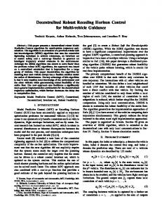
Figure 2.1: Images of the Cygnus loop: Hubble Space Telescope image at 0.7µm (left), image taken from the ground without AO (centre), the image at 1.6µm as obtained with laser guide star Adaptive Optics on the 6.5-m Multiple Mirror Telescope (right). This image is adopted from [51]. Adaptive optics compensates for atmospheric turbulence in real-time and improves the image quality of ground-based telescopes (see Fig. 2.2). In ground-based astronomy, an estimate of the wavefront error is typically obtained from a wavefront sensor. The estimate is then used to create a counter wavefront, for example, using a deformable mirror to remove the error from the incoming wavefronts [88]. A typical Adaptive Optics system consists of: 1. A wavefront sensor (WFS), which measures distortions introduced by the turbulent atmosphere; 2. A deformable mirror (DM), which corrects instantaneous wavefront distortions; 3. A control computer (CC), which tracks zero reference (at wavefront) and generates inverse distortions for actuators of the deformable mirror from the wavefront sensor's data.

Figure 2.2: Components of a typical Adaptive Optics system.

These components typically operate in a closed-loop feedback: measuring, adjusting, and estimating the residue correction, and hence compensating for atmospheric turbulence, as seen in Fig. 2.1. The main components of AO systems are described in the following subsections.

12


2.1

2.1.1 Wavefront Sensing The goal of a wavefront sensor (WFS) is to sense the wavefront with enough resolution for real-time compensation. WFSs for adaptive optics have evolved dramatically from family kitchen-made [89] lenslet arrays to sophisticated modern devices [90]. However, no ideal" WFS exists yet. In general, WFSs consist of the following main components:

• An optical device that transforms aberrations into light intensity variations; • A photosensor that transforms light intensity into an electrical signal; • The algorithm that reconstructs the wavefront. Several devices and measurement techniques allow estimation of the wavefront curvature from wavefront measuring. The most ecient and widely used wavefront sensors are described below.

2.1.1.1

Shack-Hartmann wavefront sensor

A well-known Hartmann test [91], initially devised for telescope optics control, has been adapted for use in AO systems. In the late 1960s, Shack and Platt [92] modied a Hartmann screen by replacing the apertures in an opaque screen with an array of lenslets.

Figure 2.3: Principle of the Shack-Hartmann wavefront sensor. The principle of the Shack-Hartmann (SH) wavefront sensor (WFS) is the following. An image of the exit pupil is projected onto a lenslet array (see Fig. 2.3). Each lens takes a small part of the aperture (sub-aperture), and forms an image of the source. When an incoming wavefront is planar, all images are located in a regular grid dened by the lenslet array geometry. As soon as the wavefront is distorted, images become displaced from their nominal positions. Displacements of image centroids in two orthogonal directions x, y are proportional to the average wavefront slopes in over the sub-apertures. The wavefront is proportional to the dierence between the reference centroids coordinates xrk , yrk (at light eld, reference wavefront) and the turbulent centroids coordinates

xck , yck (turbulent light eld), as shown in Fig. 2.4. For a sampled light intensity image Ii,j , positions of the centroid spots xk , yk are calculated as:


2.1

∑ xk =

i,j

xi,j,k Ii,j ∑ , Ii,j i,j

∑ yk =

i,j

yi,j,k Ii,j ∑ , Ii,j

13

(2.1)

i,j

for each k -th lenslet. The local direction angles βx and βy are computed from (2.1) as:

βx ≈ (xrk − xck )

Ly Lx , βy ≈ (yrk − yck ) , f f

(2.2)

where Lx is a size of the lenslet and f is the focus length of the lenslet. This is the Centre of Gravity (CoG) method. However, more ecient methods of centroiding have been proposed [9396]. A good feature of the Shack-Hartmann WFS is its achromaticity: the slopes do not depend on the light's wavelength. Another advantage of the Shack-Hartmann sensor is its ability to simultaneously determine x and y slopes. However, problems arise for the control computer: the computational complexity required for the wavefront slopes estimation increases as

N 2 , where N is the number of subapertures.

One feature that makes the

Shack-Hartmann wavefront sensor so use- Figure 2.4: The scheme of centroiding in a ful is that its precision and accuracy can Shack-Hartmann wavefront sensor. be scaled over a huge range depending on the choice of lenslet array and photosensor.

2.1.1.2 Summary for wavefront sensors Wavefront sensors provide the essential data about the atmospheric turbulence in AO, and each type of a WFS has its own benets. Wavefront sensors are a major source of noise and inevitable delays. The noise comes from a CCD/CMOS photosensor1 inside the WFS, and the statistics of noise depends on light conditions and the sensor type. For some cases, such as low-light operation and a fast frame-rate, the statistics is not Gaussian [98], which is important for state estimators in modern controllers. Furthermore, WFS are a major source of time-delays due to the exposure time and centroiding time of the acquired images. Shack-Hartmann WFS was chosen for the study in this research project for its eectiveness, good balance of features, and predictability of results. A Shack-Hartmann WFS is robust in terms of noise in photosensors, provides predictable results, and is scalable and 1

An avalanche photodiode (APD) can be used for wavefront sensing as well. An APD is a photodiode

that internally amplies the photo-current by an avalanche process. In [97], a successful use of avalanche photodiodes in wavefront sensors for adaptive optics was reported.

14


2.1

achromatic. For these same reasons the Shack-Hartmann WFS is the most widely used wavefront sensor in AO systems for astronomical telescopes.

2.1.2 Wavefront Reconstruction The main goal of wavefront reconstruction (WFR) is to reconstruct the distorted wavefront given wavefront sensor measurements. The concept of optimal WFR was introduced in [99] and expanded by Welsh [100,101]. The dominant problem for WFR is that a large amount of data must be processed in real time. The estimation of the computational burden is proportional to the number of independent correction channels

squared.

It is important

to note that gradient measuring inevitably contains shot noise due to nite photon counts and electron noise in the detection process [50]. The methods of wavefront reconstruction are briey outlined below.

2.1.2.1

Zonal approach of wavefront reconstruction

To obtain the estimation of the wavefront slopes sx and sy , we need to multiply the measured angles-of-arrival βx and βy from (2.2) by:

sx = where k =

2π λ ,

2π 2π βx , sy = βy λ λ

(2.3)

and λ is a wavelength of observations. The wavefront slopes (sx , sy ) and

the wavefront phase φ are related as:

5x φ = sx

5y φ = sy

(2.4)

Given the measurements of wavefront slopes sx and sy , we need to reconstruct the wavefront

φ. The relationships between the slope measurements s = [sx sy ]T and the unknown wavefront phase φ are:

5 φ = Aφ = s

(2.5)

where A is the interaction matrix that depends on the selected reconstruction geometry. The least-squares solution is obtained as:

φ ≈ (AT A)−1 AT s

(2.6)

In real systems, the least-squares solution cannot be used because the matrix AT A is singular. The wavefront phase φ can be recovered using the Moore-Penrose pseudo-inverse:

φ ≈ A† s

(2.7)

Zonal wavefront reconstruction method represents the wavefront gradients as nite dierences and numerically integrates them zone-by-zone. The

reconstruction geometry

is

the relationship between positions of the slope measurements and the phase wavefront. Measured wavefront slopes can be approximated by a nite dierence [102] using several geometries, such as Fried [103], Hudgin [104], or Southwell [105] geometry.

15


2.1

For example, consider the Fried geometry in Fig. 2.5, where horizontal and vertical arrows represent positions of the slopes measurements in x and y directions, and circles represent the positions of the wavefront phase estimation. The wavefront can be reconstructed using the Fried geometry, where a slope is the average of the phase at the four corners of a square, as follows:

(φ2 + φ3 )/2 − (φ1 + φ4 )/2 , h (φ4 + φ3 )/2 − (φ1 + φ2 )/2 = , h

sx1,1 =

(2.8)

sy1,1

Figure 2.5: The scheme of (2.9) the Fried geometry.

where h = D/N , D is the diameter of the aperture and N is the number of lenslets. The wavefront is therefore obtained as:   φ1  [ ]    φ2  sx †   ≡ A†   φ =A s y  3  φ4

2π λ βx

 

2π λ βy

(2.10)

where A† is the pseudo-inverse of the interaction matrix A and φˆ is the phase estimation. The solution for the zonal approach can also be found by the Fourier method [106]. Considering the phase dierences sx and sy are calculated for some geometry (Hudgin, Fried, Southwell or other), instead of solving the least-square problem to estimate the phase φˆ = (AT A)−1 AT s using singular values decomposition or pseudo-inverse, properties of the Fourier transform can be used to calculate the phase estimation faster [107]. The overall wavefront is a sum of the Fourier transforms of x− and y− phase dierences, and the geometry of the wavefront reconstruction can be presented as: x x y y Φp,q = Hp,q · Sp,q + Hp,q · Sp,q ,

(2.11)

x and H y are spatial where Φp,q is the Fourier representation of the wavefront's phase, Hp,q p,q x and S y are the Fourier representers of the tilts lters for X and Y axis, respectively, Sp,q p,q

from the a wavefront sensor. The algorithm of the Fourier wavefront reconstruction is as follows: 1. Take the Fourier transform from the phase dierences obtained from the WFS. Dex = F{sx } and S y = F{sy }. note Sp,q p,q i,j i,j x and H y to obtain the Fourier spectrum of the wavefront 2. Apply spatial lters Hp,q p,q

Φp,q . The spatial lters will depend on the selected geometry. 3. Take the inverse Fourier transform from Φp,q to obtain the reconstructed wavefront

φ. Use the real part of inverse Fourier transform: φ = Re[F −1 Φp,q ]. The Fourier series for a zonal WFR are now widely used because of calculation speed due to the FFT algorithm [108, 109].

16


2.1.2.2

2.2

Modal approach of wavefront reconstruction

The phase in the modal approach is presented by the coecients of the Karhunen-Loeve expansion or coecients of orthogonal polynomials such as Seidel or Zernike. The general idea is to represent the wavefront as a sum of Zernike functions:

φ(ρ, θ) =

M ∑

ai · Zi (ρ, θ)

(2.12)

i=1

where Zi (ρ, θ)'s are the Zernike functions of the mode number i, φ is the wavefront to be represented as a sum of the Zernike functions, ai are the Zernike coecients, and M is the number of Zernike polynomials used. The wavefront reconstruction reduces then to determine the Zernike coecients ai .

2.1.2.3

Summary for Wavefront Reconstruction

Both the Zernike modal method and the zonal method were chosen for this research project. The results of the wavefront reconstructors are similar; however, the Zernike method is preferable since there are no additional errors due to rectangular-to-annular aperture conversion. A Shack-Hartmann sensor has

blind modes :

that is, wavefront functions that can yield

zero or very small response in the Shack-Hartmann WFS output [40]. Certain reconstruction geometries, such as the Fried geometry [103], are insensitive to chequerboard-like wae pattern phase errors. Wae mode is the movement of two adjacent actuators in opposite directions, which can be hazardous for the mirror's surface. Constrained optimal control, which is the main subject of this thesis, can be used for the wae mode mitigation via additional constraints.

2.2 Deformable Mirrors and Actuators The image quality of astronomical telescopes is degraded due to the phase and amplitude distortions. Phase uctuations in the wavefront can be measured by the wavefront sensors. Then, using deformable mirrors (DM), the wavefront distortions are compensated. The DM adjusts the wavefront with controllable optical path dierence. The optical corrector introduces an optical phase shift ϕ by producing the optical path dierence δ . The phase shift may then be expressed as ϕ =

2πδ λ ,

where λ is the light's wavelength. The phase

shift depends on path dierence δ = ∆n∆e, where ∆e is the geometrical path dierence introduced by a DM, and ∆n is the refractive index dierence that can be produced by deforming birefringent electro-optical materials.

2.2

17

Deformable Mirrors and Actuators

2.2.1 Actuators for Deformable Mirrors Actuators for deformable mirrors are of two main categories:

• Force actuators can be hydraulic or electromagnetic. Electromagnetic actuators are built in linear (voice coil) or rotational combinations (stepper motor), and used to control the surfaces of large (ø0.5 . . . 8.0 m) mirrors.

• Displacement actuators can be piezoelectric, electrostrictive or magnetostrictive. They are used in small high-speed (ø0.5 m or less) deformable mirrors. Typical discrete deformable mirror actuators are shown in Fig. 2.6.

Voice-coil actuators The electromagnetic (EM) driver consists of a coil moving in a magnetic eld driving a piston against a cylindrical spring. A permanent magnet with pole pieces is used to transmit the force to the backplate [110]. The electromechanical conversion mechanism of a voice coil actuator is governed by the Lorentz force. In its simplest form, a linear voice coil actuator is a tubular coil of wire situated within a radially oriented magnetic eld. The eld is produced by permanent magnets embedded on the inside diameter of a ferromagnetic cylinder, and arranged so that the magnets facing the coil are all of the same polarity. The voice coil actuator is a single-phase device. Application of a voltage across the two coil leads generates a current in the coil, causing the coil to move axially along the air gap. The single phase linear voice coil actuator allows direct, cog-free linear motion that is free from backlash or irregularity.

Piezoelectric actuators Piezoelectricity is the ability of some materials to generate an electric eld in response to applied mechanical strain. The eect is closely related to a change of polarisation density within the material's volume. Application of an electric eld permanently polarises piezoelectric ceramics and induces a deformation of the crystal (PZT, P b(Zr, T i)O3 ). Changes in the relative thickness are given by

∆e e

= d33 E , where

d33 is the longitudinal piezoelectric coecient (typical values of d33 = 0.3 . . . 0.8µm/kV). A typical piezoelectric material is PZT (lead zirconate titanate with the chemical formula P b[Zrx T i1−x ]O3 , 0 ≤ x ≤ 1) has a strong piezoelectric eect [50] with

∆l l

> 0.001

and hysteresis at 10 to 20%. A key parameter of the material is the piezoelectric constant

d33 , which describes the mechanic strain to the applied electric eld. The strain for an unloaded piezoelectric element is ∆l = ld33 V /l. Piezoelectric actuators are typically made from disks of thickness t stacked together, so that the stroke of complete stack of N disks is ∆z = N td33 V /t = N d33 V . PZT has a typical value of d33 ∼ 5 · 10−10 m/V . Maximum disk thickness is limited by the maximal electrical eld that can be applied to PZT before breakdown. The maximal strain achievable is ∆z/z = Eb d33 . A disadvantage of PZT is a large voltage required to obtain a useful stroke; typically about 4µm. It is well-known [111] that the piezoelectric actuators have a hysteresis that limits their control accuracy of PZT actuators. Several methods exist for describing this hysteresis in the piezoelectric actuators [112114]. The hysteresis behaviour of piezoelectric actuators,

18


2.2

Figure 2.6: Schematic cross section of typical discrete deformable mirror actuator designs: piezoelectric (PZT), electromagnetic (EM), magnetostrictive (MAG), and hydraulic (HYDR). Images taken from [110]. including the minor loop trajectory and residual displacement near zero input, are modelled by a set of hysteresis operators, including a gain and input-dependent lag [113]. In addition, an ellipse-based mathematical model has been developed to characterise rate-dependent hysteresis [115].

2.2.2 Types of Deformable Mirrors The faceplate of a deformable mirror is made from a low-expansion material such as quartz of Corning ultra-low expansion (ULE) glass. The material for the faceplate and baseplate is the same in order to match thermal properties. Deformable mirrors have a two step design: a rst-order design with analytical expressions, and a more rigorous nite-element model for ne-tuning [50].

2.2.3 Current technologies for Deformable Mirrors The list below, inspired by [116], presents the key details and the most important characteristics of modern DMs.

Continuous face-sheet mirrors. Discrete axial piezoelectric (PZT) or electrostrictive (PMN) actuators produce a local displacement of the substrate. A deformable mirror is a thin glass sheet with bonded actuators. A modal response with a very large number of actuators is possible. The shape of the mirror is given by the expression:

r(x, y) =

∑

Vi ri (x, y)

i

where Vi is the voltage applied to the i-th actuator and ri (x, y) is the i-th inuence function. The key characteristics of continuous face-sheet deformable mirrors are:


2.2

19

• Number of actuators: up to 1000, potentially up to 100000

• Inter-actuator spacing: 2-10mm; • Electrode geometry:

rectangular

or hexagonal;

• Voltage: a few hundred Volts; • Stroke (depends on actuators): up to 10µm;

• Resonant frequency: a few kHz; • Cost: high.

Membrane mirrors. Membrane mirrors with global curvature are controlled by an array of electrostatic actuators. The shape of the mirror is given by the expression:

O2 r(x, y) =

q(Vi ) , q(Vi ) ∼ (Vi2 (x, y)) D

where q is the voltage-dependent distributed loading and D is the coecient describing the exural rigidity of the membrane. The key characteristics of Membrane deformable mirrors are:

• Number of actuators: up to 103 , increasing the number of actuators reduces the stroke per actuator;

• Electrode geometry: rectangular or hexagonal;

• Voltage: a few hundred Volts; • Stroke: a few microns, limited by the mirror curvature and the actuator size.

• Resonant frequency: several kHz; • Cost: moderate.

Bimorph mirrors. Local curvature of the mirror is controlled by sheets of piezoelectric material bonded to a thin mirror (e.g., two piezoelectric wavers bonded together with an array of electrodes between them). The front surface acts as a mirror, and the shape of the mirror is given by O4 r(x, y) = −AO2 V (x, y), where A is the constant related to the properties of the piezoelectric material (A ∝ d13 ), and V is the voltage distribution in the plane of the

PZT.

20


2.2

The key characteristics of Bimorph deformable mirrors are:

• Number of actuators: 13 - 85 ; • DM size: 30 - 200 mm; • Electrode geometry: radial; • Voltage: few hundred Volts; • Stroke: few microns; • Resonant frequency: more than 500 Hz;

• Cost: moderate.

MEMS (micro-electromechanical systems) mirrors. MEMS-based DMs are made by micro-lithography and semiconductor batch processing. Small mirror elements are deected by electrostatic forces. The overall prole of the DM is directly controlled by an array of micro mirrors. The remaining problems of DMs utilising current MEMS technology are: insucient stroke, elements are too-small, scattering, diculties with multilayer coating, and diculties with integration of large arrays of high-voltage drivers. The key characteristics of MEMS mirrors are:

• Number of actuators: up to 105 −106 ; • Electrode geometry:

rectangular,

hexagonal, and others;

• Voltage: several Volts: • Stroke: up to several µm; • Response time: expected to be less than 10µs;

• Cost: potential to be very inexpensive, estimated at $10 per actuator.

Segmented mirrors. In segmented mirrors, smaller independent elements are actively controlled by the actuators to conform to the mirror's shape. Segmented mirrors are comprised of separate segments with small gaps between each segment. Segmented mirrors are usually used for large mirrors.


2.2

21

The key characteristics of segmented deformable mirrors are:

• Number of actuators: up to 100; • Elements geometry: sector-shaped segments or hexagonal segments;

• Control signals: depend on the actuator type, but precision electromechanical drivers are typically employed;

• Stroke: may be as large as needed; • Response time: several hundred ms; • Cost: very high.

Liquid crystal modulators. Phase modulation stems from the orientation of the liquid crystal molecules in the presence of an applied electric eld. Phase prole is determined by the orientation of the liquid crystals molecules controlled by an applied electric eld. Typically, the amplitude of the phase shift does not exceed 2π and the mirror operates in a "wrapped" mode. The key characteristics of liquid crystal modulators are:

• Electrode geometry: rectangular or hexagonal;

• Voltage: ∼ 10 Volts at a frequency of several kHz;

• Eective stroke: one λ to several λ (light wavelengths, ∼ 0.400 − 1µm);

• Response time: typically > 10ms; • Polarization sensitive, strong dispersion, slow response, temperature sensitive.

• Cost: moderate as the technology is similar to LCDs, potentially inexpensive;

Ferrouid mirrors. Ferrouids are liquids that contain a suspension of ferromagnetic particles. In the presence of an external magnetic eld, the magnetic particles align themselves with the eld and the liquid becomes magnetised [117]. For a ferrouid surface at rest in the plane z = 0, the equation that describes the ferrouid surface amplitude h under the applied magnetic eld is given by [118]:

22


h(x, y) =

2.2

µr − 1 [B 2 (x, y) + µr Bt2 (x, y)] 2µr µ0 ρg n

where ρ is the density of the ferrouid, µr the relative magnetic permeability of the ferrouid, and Bn and Bt are the normal and tangential components (relative to the x − y plane) of the external magnetic eld [119]. Each actuator is made of about 200 loops of

ø0.3 mm copper wire . The eective external diameter of an actuator is 5 mm [119]. The key characteristics of Ferrouid mirrors are:

• Number of actuators: 100-1000 (e.g. a 2-inches diameter ferrouid DM can have more than 450 actuators);

• Electrode geometry: rectangular, circular;

• Voltage: several Volts: • Current: 10-100 mA : • Stroke: the maximum surface amplitudes achievable with ferrouids are limited by the so-called Rosensweig instability. Typically several µm;

• Response time: mirror can be driven at a frequency of 40 Hz

• Cost: moderate, estimated at $100 per actuator [119].

2.2.4 Desirable parameters of Deformable Mirrors Astronomical AO systems require a large variety of deformable mirrors with challenging parameters [6]. Even an 8 m telescope can require up to 5000 actuators, with this number increasing up to 250 000 for Extremely Large Telescopes (ELT). A summary of parameters, adopted from [6], is provided in Table 2.1 The required stroke for the actuators in a deformable mirror is generally given as

5 − 10µm. For high-order corrections, the bandwidth must be of the order of 1 kHz. For a smooth overall shape of the surface with low residual errors, the inter-actuator coupling [6] should be 20-30%.

2.2.4.1

Summary for the Deformable mirrors

Deformable mirrors dene the dynamics of the AO system and the specic properties of the corresponding optimisation problem. For example, segmented mirrors do not have coupling between the segments, whereas membrane mirrors have complicated dynamics that involves

2.3

Control Strategies for Adaptive Optics Systems

23

Table 2.1: Parameters for deformable mirrors in ELT-class telescopes [from [6]].

Parameter of a Deformable mirror Required value Number of actuators Inter-actuator spacing Actuator stroke Inter-actuator coupling Bandwidth

5000 to ≥ 250000 200µm . . . 1mm 5 . . . 10µm 20 - 30 % 1 kHz

coupling between many adjacent actuators. Dierent types of DMs have dierent dynamics, and this is what motivates the study and modelling of DMs. The hardware limitations of deformable mirrors are more important, since a too-large movement of an actuator can damage the surface of a continuous-faceplate DM. This motivates the study of actuator constraints and constrained control.

2.3 Control Strategies for Adaptive Optics Systems In general, AO systems can be modelled as Linear Time-Invariant (LTI) Multi-Input MultiOutput (MIMO) systems. The goal of the control system is to compensate for distortions in incoming wavefronts, which it does by processing the data from the WFS and generating signals for the DMs. The typical criterion of eectiveness is the minimal residual phase variance of the wavefront [51].

2.3.1 Control techniques currently used in Adaptive Optics The most widely used control technique for AO systems is a simple PI [79] or PID [10] controller. Although classical control does not account for the actuators coupling in the deformable mirror and the constraints on maximum actuator movement, PI/PID controllers are still used due to their ease of implementation and the fact that in good seeing conditions, PI controllers are generally considered to be good enough [5]. More advanced controllers, such as Linear Quadratic Gaussian (LQG) and minimum variance [27, 120] controllers have been also considered. LQG controllers have been designed [5, 13] and simulated [14, 15] for adaptive optics. The experimental validation of optimal control was shown to outperform classical control [18, 19]. Robust control has also been discussed [4, 2022], simulated [24], and tested [25] for adaptive optics applications. Adaptive control for adaptive optics has also been considered [28, 29].

2.3.2 Proposed control strategy: constrained Receding Horizon Control All the aforementioned control techniques are unconstrained, whereas the actuators in deformable mirrors are obviously constrained by a maximum allowable movement. Too large control signals can cause damage to the surface of DMs.

24

2.3


The main motivation for using constrained Receding Horizon Control (RHC) is to provide a control signal that is optimal

within the imposed constraints,

to prevent the

damage to the surface of a DM. Therefore, RHC provides the means for intelligent handling of constraints and dynamics, making it possible to use adaptive optics even in strong turbulence conditions. The constrained RHC technique remains relatively unexplored in adaptive optics [33 35, 37]. It has been used [33] to control a Thermal Deformable Mirror to correct static aberrations in a light beam. The consecutive line searches method [38] in the direction of several Zernike modes was used in [33]. The Nelder-Mead [39] algorithm was used in [34] for correction of optical aberrations in a closed-loop feedback.

2.3.3 Alternative Solutions and Approaches for Constrained Control Other possible solutions include switched controllers for constrained and unconstrained cases separately.

One of the solutions to the over-saturation problem is to use con-

troller switching methods, such as multi-mode regulators [121] or piecewise-linear control (PLC) [122], to deal with input constraints. A common feature of these strategies (and PLC in particular) is that these schemes yield relatively low gain controllers to ensure that the input constraints are avoided. These methods are conservative since the control is away from the constraints [123]. However, the analysis of stability of switched systems is far from obvious [124127]. While PLC is an interesting approach and can be considered for low-dimensional systems, it is too cumbersome for high-dimensional coupled control systems. Further, PLC yields lower-gain control and therefore does not use the full potential of control. An attractive feature of an online QP is that, even for large systems, it will make possible decision

the best

in both constrained and unconstrained cases, thus providing high-gain

control without the risk of over-saturation and abrupt changes of control inputs.

2.3.4 Receding Horizon Control for Adaptive Optics The main reason to apply Receding Horizon Control (RHC) in adaptive optics is to account for the inevitable hardware constraints of deformable mirrors: actuators are constrained by a maximal allowable movement, and the controller must generate a signal that is optimal within constraints. Doing otherwise will lead to inferior performance and a risk to the DM's surface. RHC solves an optimisation problem at each sampling instant to generate the best possible control signal for the deformable mirror and therefore to compensate for the atmospheric turbulence. The basic idea of Receding Horizon Control, as illustrated in Fig. 2.7, is to make a plan of the future control signals N steps forward. An optimisation algorithm (1) computes the optimal strategy within prediction horizons (N steps ahead) and constraints, then (2) executes the rst control move, before (3) moving the prediction horizon one step further and re-planning [128]. Using the Measured Output and comparing it with the Reference Trajectory (see Fig. 2.7), Receding Horizon Control produces the Predicted Output control signal. This is why only the rst signal is applied:

25

Optimisation strategies for RHC in AO

2.3

Figure 2.7: The Receding Horizon Control scheme. on the next sampling instance the control signal is recalculated, as Receding Horizon Control constantly adjusts the control moves based on the most recent information [129]. The prediction horizon is continually shifted forward; hence the name

receding

horizon

control. The derivation of RHC is provided in Chapter 3. The essential ingredient of constrained RHC is an optimisation algorithm that actually solves the control problem online. However, the optimisation problem can be formulated dierently, such as Quadratic or Linear Programming. The next section introduces a comparison of the two formulations, along with their benets and shortcomings.

2.4 Optimisation Strategies for Receding Horizon Control in Adaptive Optics An article entitled Who needs

QP for linear MPC anyway?

appeared in Automatica [130]

and discussed the pitfalls and benets of Linear Programming algorithms compared to Quadratic Programming. The following short section, inspired by insightful discussions in the book by Jan Maciejowski [131], discusses the advantages of Quadratic Programming and its benets for Receding Horizon Control.

2.4.1 Quadratic and Linear Programming Optimisation problems are usually solved numerically by going downhill. However, many optimisation problems have local minima, and the algorithm might become stuck at such a local minimum, unaware that the true global minimum is elsewhere [131]. The optimisation problem being discussed in this thesis is a set is

convex

smooth,

or

convex.

Simply speaking [38],

if every point in the set can be seen from every other point, along an

unobstructed straight path between them, where unobstructed means lying in the set. An objective function is convex if the straight line joining any two points on the cost surface is never below the surface. Due to the convexity of the objective function, there is only one minimum, thus it is guaranteed that a global minimum will eventually be reached if one keeps going downhill [131]. The optimisation problem of optimal control can be formulated as a Linear or a Quadratic Program.

26

2.4


A Quadratic Program (QP) is an optimisation problem of the form: minimise θ

1 T θ Hθ + FT θ 2

subject to Ωθ ≤ γ The problem is convex if the Hessian matrix is positive semidenite H 0. Since the constraints are linear inequalities, the surfaces on which they are active are

hyperplanes.

The constrained objective function can be visualised as an ellipsoid surface, parts of which have been cut o by a number of at faces. It is clear that this constrained surface remains convex [131].

A Linear Program (LP) is the special case of a QP when H = 0: minimise θ

FT θ

subject to Ωθ ≤ γ The objective function is also convex, and the minimum always occurs at a vertex. The constrained objective surface can be visualised as a surface with at faces (simplex) [132, 133].

2.4.2 Optimal Control Problem Formulation: Linear or Quadratic? It is possible to modify the cost function used in constrained optimal control, so that absolute values, rather than squared values, of errors are penalised. One of the historical reasons for adopting such a formulation is that LP problems can be solved more quickly than QP problems, and that there is more experience of solving LP problems. The importance of this reason is decreasing rapidly because of the eorts being made in the development of algorithms for solving QP problems. Another reason for adopting the QP formulation of the constrained control problem is that

2.4.2.1

the resulting behaviour is dierent.

Linear and Quadratic Programming formulations: dierence in behaviour of a solution

The solutions of LP problems are always at the intersection of constraints, occasionally on a single constraint. The solutions of QP problems can be o constraints, on a single constraint, or (relatively rarely) at an intersection of constraints, as seen in Fig. 2.8. Consider a problem with only two decision variables x1 and x2 . In Fig. 2.8, adapted from [131], the thick solid lines represent linear inequality constraints, the feasible region is the interior of the region bounded by these lines. The dashed lines represent constant cost contours, those for an LP problem being shown on the left (straight lines, or

hyperplanes

in general) and

those for a QP problem being shown on the right (ellipses, or

hyper-ellipsoids

in general).

For the LP problem, the cost increases as one moves upwards in the gure, and for the QP problem the cost increases as one moves out from the centre of the ellipse.

2.4

Optimisation strategies for RHC in AO

27

Figure 2.8: Cost contours and constraints for the LP (left) and QP (right) problems. The black dots show the optimal solution. It can be seen from Fig. 2.8 (on the left), that the optimal solution to an LP problem must always lie on at least one constraint. The solution is relatively robust with respect to the cost function: the slope of the cost contours can vary quite a lot before the optimal solution changes. But when it does change, it jumps suddenly to one of the other corners of the feasible region. The gure on the right in Fig. 2.8 shows that the optimal solution to a QP problem behaves dierently: the optimal solution is on one of the constraints. However, there can be situations when the centre of the ellipse is in the interior of the feasible region, and then the solution will not be on any of the constraints. In this case the optimal solution is completely insensitive to changes in the constraints if it is in the interior of the feasible region, but depends continuously on the cost function. If it is on the boundary of this region - that is, some constraints are active - then it depends continuously on both the cost function and the constraints.

2.4.2.2 Issues with Linear Programming in Constrained Control The comparison of the closed-loop responses between a linear (or l1 ) criterion and a quadratic criterion [134] indicates that the l1 formulation forces the state to the origin in nite time as opposed to the quadratic programming formulation, where the state exponentially approaches the origin. Forcing the state to the origin in nite time is appealing for servo regulation. However, a dead-beat control may yield poor closed-loop performance in process control applications, becoming especially evident in the presence of state noise. Recently Dave [135] has advocated the use of an l1 and l∞ norm as a performance criterion for RHC. The solution of a linear program is less computationally demanding than the corresponding solution of a quadratic program of the same size and complexity. Thus it may be preferable to formulate RHC as a linear program [134]. However, it was found that the l1 formulation may result in dead-beat performance or idle control performance (i.e., no control action) when the input penalty matrix R is large relative to the matrix

Q. Extensive numerical simulations in [136] show that the idle control policy in the l1

28


2.5

formulation appears to be common, which represents potential problems for closed-loop operations.

2.4.3 Which optimisation formulation is preferable for Adaptive Optics? Each of the formulations - Linear or Quadratic Programming - has its own benets. The main consequence of the l1 criterion is that it may yield either dead-beat or idle control responses. Both of these types of responses may be unsuitable for process control applications [136]. Thus, it can be concluded that the Linear Programming formulation of RHC is not suitable for adaptive optics systems, since the performance issues raise questions concerning the suitability of the l1 criterion for RHC. Therefore, we choose the Quadratic Programming formulation of an optimisation problem for the control of adaptive optics systems.

2.5 Chapter Summary This chapter has introduced the key concepts of Astronomical AO and motivates further developments as follows:

À Optimal control for AO systems is a logical choice. The numerical issues and poor performance of Linear Quadratic Regulator in high-gain mode are far from obvious. This motivates the transition from Innite to Receding Horizon Control in Chapter 3.

Á In justifying the choice of the QP formulation for this research project, it has been explained that the QP formulation of the optimisation problem for adaptive optics control oers more exibility than the LP formulation.

Â The control problem of a DM with coupled actuators has a particular matrix structure, which can be analysed and exploited to accelerate further the online QP solution in Receding Horizon Control. This is the main topic of Chapter 4.

Ã Tight computational speed requirements in AO are the main motivation for the detailed study of optimisation algorithms in Chapter 5.

Ä Development of fast optimisation algorithms in Chapter 5 and an insightful structure analysis in Chapter 4 provide the basis for a comprehensive numerical study of the feasibility of constrained RHC in AO in Chapter 6.

Å As will be shown in Chapter 6, Receding Horizon Control can be computed very quickly in adaptive optics, but is it worth the eort? The answer to this important question in terms of disturbance rejection performance is given in Chapter 7. This project has a considerable potential for further work, as indicated in Chapter 8.

¦

Chapter 3

Optimal control for Adaptive Optics: from Innite to Receding Horizon The greatest diculties lie where we are not looking for them.

F

Johann Wolfgang von Goethe

ormulation of Innite and Receding Horizon Control for Adaptive Optics sys-

tems is the main topic of this chapter. The dynamic model of adaptive optics components is the subject of Section 3.1. The formulation of Innite Horizon

Control (or Linear Quadratic Regulator) along with its strong and weak points is provided in Section 3.2. The potential numerical problems of the LQR control and the motivation

for the transition from Innite to Receding Horizon Control are discussed in Section 3.3. The constrained control formulation as an optimisation problem and the benets of such a formulation are addressed in Section 3.4. Finally, the results of an initial assessment of constrained Receding Horizon Control for adaptive optics are presented in Section 3.5.

3.1 Dynamic models of Adaptive Optics components An adaptive optics system can be considered as a Linear Time-Invariant (LTI) MultiInput Multi-Output (MIMO) system that consists of a wavefront sensor, a controller, and a deformable mirror (DM) for the real-time compensation of an output disturbance (atmospheric turbulence). The system is subject to both output disturbance and measurement noise from the photosensor inside the wavefront sensor. The goal of the controller is to track a zero reference, which is a at wavefront.

3.1.1 The model of a wavefront sensor The dynamics of the wavefront sensor (WFS) is described by the integration time Tf of the photosensor, since the output of the sensor is an average of the signal from t to

t + Tf . An additional delay for data processing and reconstruction is denoted by τwf s . In 29

30

Chapter 3: Optimal control for Adaptive Optics

3.1

the discrete-time equivalent, the dynamics of the WFS are usually represented by sensor delays proportional to Tf + τwf s .

3.1.2 Dynamic Models of Deformable mirrors The dynamics of the actuators in a deformable mirror (DM) is considered to be a rst-order transfer function (TF) with a fast pole [50, 137], which agrees with experimental data obtained via system identication from the hardware optical testbench [138]. The dynamics of DM actuators usually dier between actuators. To account for this variation, the continuous Transfer Matrix (TM) is generated in this work taking the values of the poles from a ( ) Normal Distribution pN ∼ N p, σp2 with mean p and standard deviation σp = α · p to make each actuator's TF slightly dierent (α is considered as α = 0.01). The

Figure 3.1: A deformable mirror with piezoelectric actuators that control the shape of the surface (uncoated).

continuous TF for the (i, i)-th actuator is therefore:

G(s)i,i plant =

1 , s + pN

(3.1)

where the mean value of the poles is p = 1500. This kind of dynamical model, with coupling between the four nearest actuators, was found adequate [138, 139] for the target hardware, which was a Xinetics deformable mirror (see Fig. 3.1) with 37 actuators arranged in a 7 × 7 square grid, spaced at 5 mm intervals between each actuator. The mirror's surface is ø30 mm, made of an ultra-low-expansion (ULE) glass.

3.1.3 Coupling models for actuators in Deformable Mirrors Actuators are arranged in a square grid and attached underneath the reective surface of a deformable mirror. The faceplate of the mirror is made from a low-expansion material such as quartz of Corning ULE. When an actuator is energised (pushed up or pulled down), it displaces neighbour actuators due to the sturdiness of the mirror's surface. Therefore, one energised actuator aects its neighbouring actuators to some extent, increasing the complexity of dynamics of a deformable mirror. This is called

inter-actuator coupling.

In this study, three cases of coupling between the actuators in a deformable mirror are considered, as shown in Fig. 3.2: 1. no coupling between the actuators, when the energised actuator has no eect on its neighbours (Fig. 3.2(a));

31

Dynamic models of Adaptive Optics components

3.1

2. coupling between nearest neighbour actuators, when the energised actuator aects only its four nearest neighbours (see Fig. 3.2(b)); 3. coupling between nearest neighbours and diagonally adjacent actuators, when the energised actuator aects its four nearest neighbours

and

four diagonally

adjacent actuators (see Fig. 3.2(c)).

(a)

(b)

(c)

Figure 3.2: Coupling cases for the DM models: (a) decoupled case; (b) coupling between nearest neighbours; (c) coupling between nearest neighbour and diagonally adjacent actuators. The coupling between neighbouring actuators in a deformable mirror is modelled as follows. Denote γ ∈ (0, 1) the value of the coupling

degree

between their neighbour actuators.

The strength of inuence of one actuator on its neighbours depends on the mechanical properties of the mirror's surface, inter-actuators spacing and number of actuators: the closer the actuators are to each other, the more an energised actuator aects its neighbours. Actuators coupling can be described as a proportional relationship between the actuators' transfer functions and described by a coupling degree γ . The transfer matrix therefore contains o-diagonal elements Gi,j :



G1,1 G1,2

0

 M G G2,2 G2,3 GTplant (s) =   2,1 .. .. .. . . .

G1,4 0

0

...



 G2,5 . . .  . 

(3.2)

For this example of a 3 × 3 actuators grid (9 actuators), the coupling transfer function

G5,2 (s) between actuator 5 and actuator 2 is obtained as G5,2 (s) = γ · G5,5 (s), where γ is the coupling degree. Continuous-faceplate DMs usually have a relatively strong coupling [6] between the nearest neighbour actuators such as 20-30% (i.e., γ = 0.20.3) with interactuator spacing 0.21 mm and strokes of up to 10µm.

3.1.3.1 No coupling between the actuators The decoupled case corresponds to segmented mirrors, where the segments move independently from each other and do not interact. The tip-tilt mirror is mounted on a piezo-driven tilting stage. The stage tilts horizontally and vertically according to voltages applied to two piezo-devices [140]. When the actuators do not inuence each other, the Transfer Matrix (TM) contains only diagonal terms and all o-diagonal transfer functions are zeros

32

3.1


(e.g., G1,2 (s) = 0, which describes the interaction between actuator 1 and 2). The TM is as follows:

  G1 (s) =  

G1,1

0

...

0 .. .

G2,2 .. .

..

 0 ..  .  

(3.3)

.

Early AO systems seemed to ignore the coupling [45] between the actuators, leading to decreased performance in terms of atmospheric turbulence compensation. Therefore, models of the deformable mirrors that are more realistic need to be considered.

3.1.3.2

Coupling between nearest neighbour actuators

A more realistic model of the continuous-faceplate DMs includes the coupling between nearest neighbour actuators, as shown in Fig. 3.2(b). Here the energised actuator 5 aects actuators 2, 4, 6 and 8. Continuous-facesheet deformable mirrors usually have relatively strong coupling only between nearest neighbour actuators (i.e., the four closest actuators to the energised one). When the coupling is between nearest actuators, the transfer matrix becomes denser (below, the bold font shows the activated, or energised, actuator's TF, for a 3 × 3 actuator grid):







G1,1

0 γ 0    G Υ2 =  γ 1 γ  , G2 (s) =   2,1 .. 0 γ 0 .

G1,2

0

G2,2 G2,3 .. .. . .

G1,4 0

0

0

G2,5 0

... 0



 ... 0   .. .

(3.4)

where γ ∈ (0, 1) is the value of the coupling degree between the nearest neighbour actuators only, as seen in the coupling matrix Υ2 .

3.1.3.3

Coupling between nearest and diagonally adjacent actuators

When the actuators are spaced closely to each other in a continuous-faceplate deformable mirror, the coupling between the actuators also includes the diagonal adjacent actuators, making the DM's dynamics more complex. When the coupling is between nearest actuators and

diagonally adjacent actuators, the TM becomes denser:



γ2 γ1 γ2

 Υ3 =  γ1

1

γ2 γ1





G1,1

  G γ1  , G3 (s) =   2,1 .. γ2 .

where γ ∈ (0, 1) is the value of the

G1,2

0

G2,2 G2,3 .. .. . .

coupling degree

G1,4 G1,5 0

0

G2,5 G2,6

... 0



 ... 0   .. .

(3.5)

between the actuators. These matrices

are presented for an example of a 3 × 3 actuators grid. The activated (energised) actuator's transfer function in (3.5) is emphasised by a bold font. In this case, the coupling matrix Υ3 contains the coupling degree γ1 for the nearest neighbours (four closest actuators aected by the energised one) and γ2 for the diagonally adjacent actuators. The coupling degree

Dynamic models of Adaptive Optics components

3.1

33

for the diagonally adjacent actuators is usually lower (depending on the type of mirror used).

3.1.4 Typical sampling rate of an Adaptive Optics system Wavefront sensor integration times may be shorter than 1 millisecond [141] due to high bandwidth requirements for the control loop [142] in astronomical adaptive optics systems. Therefore, choosing the sampling frequency results in trade-os [143], including: 1. Atmospheric turbulence to correct for. The system bandwidth has to be larger than the turbulence temporal evolution of the faster mode to be corrected. 2. The system parameters, including detector technologies, correcting devices, and real time computer performance. A consequence of this, which is important for constrained control, is that the turbulence does not change much from one sampling instance to the next in the case of fast sampling rates.

3.1.5 Output disturbance dynamics The output disturbance in adaptive optics systems is caused by atmospheric turbulence. It was shown in [144] that an autoregressive model AR(1) provides limited performance due to the nature of the approximate model. An AR(5) model leads to a loss of performance because of the increased sensitivity to variations of temporal characteristics of the atmospheric turbulence. An AR(2) model provides a reasonable agreement with the Kolmogorov model [145] in good seeing conditions and is used in this work in the following form (before time discretisation):

G(s)atm i,i =

1 . s2 + s · κ 1 + κ 2

(3.6)

The poles of the output disturbance model are usually slower than the poles of the DM. In this study we used κ1 = 2 and κ2 = 30 as values for the coecients for (3.6).

3.1.6 The complete model of an Adaptive Optics system The complete model of the system consists of WFS dynamics, actuators of the DM, and a M (s), time delay of the wavefront sensor. The continuous transfer matrices of the plant, GTplant

and the disturbance, Gatm (s), were formed using (3.1) and (3.6) . These transfer matrices were converted to the state space formulation, discretised using a zero-order hold (ZOH) on the inputs with a sample time of Ts = 10−3 seconds to obtain the state space matrices of the overall model.

34

3.2


3.2 Formulation of Linear Quadratic Gaussian control for Adaptive Optics This section provides the formulation of the Linear Quadratic Regulator (LQR) for Adaptive optics. The Kalman lter is used in this work as a state estimator, comprising a complete Linear Quadratic Gaussian (the Regulator and the Kalman lter) controller. The system model considered is a Linear Time Invariant system subject to output disturbances.

3.2.1 Linear Quadratic Gaussian control for Adaptive Optics The system is assumed LTI with states x[k], inputs u[k], and measurements y[k] as:

x[k + 1] = Ax[k] + Bu[k] + Gξ[k]

y[k] = Cx[k] + Du[k] + η[k]

(3.7)

here ξ[k] is the process noise and η[k] is the measurement noise. The matrices A, B , and

C must be augmented to account for the plant dynamics and the output disturbance: [ A=

Aplant

0

0

Aatm

]

[ ,B =

Bplant 0

]

[ ,G =

0 Batm

] , C = [Cplant Catm ], D = 0 (3.8)

M (s), and the These matrices are obtained from the Transfer Matrices of the plant, GTplant

disturbance, Gatm (s), from (3.1) and (3.6). The Strehl ratio is typically used to derive a performance criterion for the controller. The Strehl ratio is the ratio of the peak intensity of a measured point spread function (PSF) to the peak intensity of a perfect diraction-limited PSF for the same optical system. The Strehl ratio values are S ∈ [0, 1], and the closer S is to 1, the better (sharper) is the image. The objective of the controller is to minimise the wavefront phase variance (i.e., to keep the wavefront at), which is equivalent to the maximisation of the Strehl ratio. The cost function for the innite-horizon control problem can be formulated as:

) ∞ ( ∑ 1 T 1 T J= x Qx + u Ru 2 2

(3.9)

k=0

The matrix Q can be chosen as Q = C T C , and the matrix R can be set as R = 10−12 I to meet the performance requirements of an AO system. In the time-invariant innite horizon problem, it is well-known that the solution stabilises the system.

3.2.1.1

State feedback gain evaluation

The feedback gain can be found using the solution of the discrete-time algebraic Riccati equations (DARE):

AT ΩK A − AT ΩK B(B T ΩK B + R)−1 B T ΩK A + Q = ΩK

(3.10)

Formulation of LQG control for AO

3.2

35

The solution of the DARE in (3.10) is the matrix ΩK , which is used for the state feedback gain calculation:

Kgain = (B T ΩK B + R)−1 B T ΩK A

(3.11)

where Q = C T C = [Cplant Catm ]T [Cplant Catm ] and R = 10−12 I . The matrix Q contains zeros on the main diagonal, which may cause problems with nite precision computations for the DARE solvers (see Subsection 3.2.3 for a discussion of this issue).

3.2.1.2 State observer gain evaluation The observer gain (the Kalman lter) is found from the dual DARE:

AΩL AT − AΩL C T (CΩL C T + W )−1 CΩL AT + V = ΩL ,

(3.12)

where V = GGT and G = [0, Batm ]T , as indicated in (3.8). Using the solution ΩL of the DARE in (3.12), the observer gain can be evaluated:

Lgain = AΩL C T (CΩL C T + W )−1

(3.13)

where W is the covariance matrix of the measurement noise.

3.2.2 Formulation of Linear Quadratic Gaussian control By combining the solutions for the feedback and the observer from the previous subsections, the controller can be formulated as:

u[k] = −Kgain x ˆ[k] x ˆ[k] = Aˆ x[k − 1] + Bu[k − 1] + Lgain (y[k − 1] − C x ˆ[k − 1]).

(3.14)

In numerical experiments, the LQR/LQG controller is used in the form of (3.14).

3.2.3 Numerical issues of the optimal control for Adaptive Optics systems A typical DM for the AO system may consist of thousands of actuators, such that the matrices of the LQR controller can be very large. Although most of the calculations are performed o-line, the evaluation of the control matrices can be dicult due to the nite precision of the computations. There may be numerical problems in solving the corresponding DARE for the LQR due to augmentation of the state matrices to account for delays and/or atmospheric turbulence. This may explain many of the problems that authors [146] have encountered in trying to solve the Riccati equations for ELT-size telescopes. This issue is considered in the subsections below. In the standard LQR formulation, the weight matrix Q = [Cplant Catm ]T [Cplant Catm ], which is used in the cost function in (3.9), may become ill-conditioned. This may cause problems with nite precision computations for the DARE solvers. The matrix elements that correspond to the output disturbance can be small compared to the plant elements

36

3.2


(see Fig. 3.3(a)). The determinant of the matrix Q for the solution of Riccati equation can be close to zero and in turn leads to numerical problems in solving the Riccati equations. 1

1

0.8 10

0.8 10

0.6 20

0.6 20

0.4 30

0.2

0.4 30

0.2

0 40

0 40

−0.2 50

−0.2 50

−0.4 60

−0.6

−0.4 60

−0.6

−0.8 70

−0.8 70

10

20 30 40 50 60 Total elements=5625, nonzero=100 (98% sparse)

70

−1

(a)

10


−1

70

(b)

Figure 3.3: The structure of the LQR matrices: (a) matrix Q from (3.9); (b) matrix V = GGT from (3.12). Consider the singular value decomposition (SVD) of the matrix Q as Q = U ΣV H , where Σ is the diagonal matrix of singular values %i . Dene the

condition number

[147]

as κ(Q) = %max /%min . Even in the case of no time delays, the condition number for the matrix Q is of order κ(Q) ≈ 5 · 1015 for the 5 × 5 actuator model (this value is obtained with diagonal loading of 1 eps, see Subsection 3.2.3.1). This is not a surprise since the matrix Q contains many zeros (or very small numbers) on the main diagonal. A similar problem occurs with the matrix V = GGT , where G = [0, Batm ]T . The matrix

V is used for the calculation of the steady-state Kalman estimator. The condition number for the matrix V is of order κ(V ) ≈ 1 · 109 for the 5 × 5 actuator model (see Fig. 3.3(b)). As before, the value is obtained with diagonal loading of 1eps, otherwise κ(V ) = +∞ since the smallest eigenvalue is zero. The solver implemented in MATLAB's DARE routine uses the QZ algorithm [148] to deate the extended symplectic pencil and compute its stable invariant subspace. In case of poor conditioning, as described above, the algorithm often terminates with errors: evaluation of eigenvalues is numerically unstable because the spectrum is too close to the imaginary axis. Augmentation of the state matrices to account for time-delays of two cycles (typical for adaptive optics systems) does not noticeably change the numerical properties of the matrices Qaug and V . However, the numerical problems with the conditioning still present: κ(Qaug ) ≈ 1 · 109 and κ(V ) ≈ 1 · 109 .

3.2.3.1

Using a diagonal loading to circumvent numerical problems

Since the condition number κ(Q) can be large, indicating possible numerical problems, regularisation of the weighting matrix Q is required. One can use the

diagonal loading

technique for the regularisation that is similar to Tikhonov regularisation [149]:

Q = Q + δI,

(3.15)

3.2

37

Formulation of LQG control for AO

where δ is the regularisation term δ = /Tf , Tf is the sampling period, is the oatingpoint relative accuracy, and I is an identity matrix. By increasing the regularisation term in (3.15) to 107 δI , the condition number κ(Q) is reduced to 105 . Reasonable values of the regularisation term δ are found to be within the range of . . . 103 .

3.2.3.2 Typical algorithm for Discrete Riccati Equation Equations The actual implementation of a DARE solver can be quite complicated and not always numerically stable. As an example of the DARE solver [148] implementation in MATLAB, DARE:

AT XA − X − AT XB(B T XB + R)−1 B T XA + Q = 0 is solved as a case of the general discrete-time algebraic Riccati equation (GDARE):

AT XA − E T XE − (AT XB + S)(B T XB + R)−1 (B T XA + S T ) + Q = 0 The actual Riccati equation is solved by the gdare function, a generalised solver for DARE. The gdare function computes the unique stabilising solution of the discrete-time algebraic Riccati equation associated with an extended symplectic pencil of the form:



A

0

 H − tJ =  −Q E T ST

0

B





E

  −S  − t  0 R 0

0 AT −B T

0



 0 , 0

(3.16)

where, S = 0 and E = I . For the evaluation of the eigenvalues, the DARE function calls

qz.m, which is a QZ factorisation for generalised eigenvalues. The limitations of the algorithm used in MATLAB's DARE is that the pair (A, B) must be stabilisable (all eigenvalues of A that are outside the unit disk must be controllable). A sucient condition for (Q, A) to be detectable is: [

Q

S

ST

R

] >0

(3.17)

Therefore, when the matrix Q has small/zero diagonal elements, the sucient condition does not hold. Furthermore, one of the assumptions is that the associated symplectic pencil (matrices in (3.16)) has no eigenvalues on the unit circle. However, due to the models of the adaptive optics system and the augmentations, both H and J matrices do

have eigenvalues that are very close to the unit circle (e.g., λ = 0.9884 + 0.0568i). This leads to the numerical problems in solving the DARE for adaptive optics.

3.2.4 Summary for Linear Quadratic Regulator control The discussions of previous sections allow to conclude that, although a Linear Quadratic Regulator seems to be attractive and a relatively straightforward control technique, its implementation for a typical adaptive optics system is not free of numerical problems.

38


3.3

This is because the numerical algorithms for solving a Discrete Algebraic Riccati Equation can be unstable in the case of fast discretisation and nite precision computations. A short summary of the properties of LQR is provided in Table 3.1 Table 3.1: Summary of the properties of Linear Quadratic Regulator for Adaptive Optics applications.

Advantages:

Disadvantages

4 Most computations (DARE solution) are done o-line; 4 LQR can handle coupled actuators dynamics.

6 Q and V matrices can be poorly conditioned; 6 DARE solvers can fail to nd a numerical solution; 6 LQR cannot eciently handle constraints; 6 System identication needed for models of DM and turbulence;

To summarise, the numerical properties of the augmented matrices Q and V (used for the state feedback and the state estimator, respectively) are prone to numerical problems. Even if these numerical problems can be alleviated by numerical tricks such as diagonal loading, a better solution could be to use an alternative formulation of the optimal control, such as Receding Horizon Control.

3.3 From Innite to Receding Horizon control The main disadvantages of Linear Quadratic Regulator are the potential numerical problems and the complexity of the algorithms for numerically solving Riccati equations. This section starts with a motivation for constrained control and provides the formulation of Receding Horizon Control as a quadratic optimisation problem.

3.3.1 Motivation for constrained optimal control in Adaptive Optics An adaptive optics system represents a signicant challenge from the control point of view. Matrices for the state space formulation are large (DMs can have more than 100×100 actuators), and usually augmented with at least two sample delays. The specic challenges are: 1. the control signal has hard constraints that cannot be violated or softened (or the mirror's surface might be damaged); 2. specic additional constraints may be required (e.g., maximum actuators movement, wae1 mode [40]); 1

Wae mode is the movement of two adjacent actuators in opposite directions, which can be hazardous

for a mirror's surface. While RHC can be used for wae mode mitigation, our preliminary simulations [150] show that it takes too long even for small adaptive optics systems.

From Innite to Receding Horizon control

3.3

39

3. limited time for computation of a control input: the QP must be solved within 1 msec or faster. However, rstly, it is worth asking: Why do we need optimal control in adaptive optics? Indeed, there were several reasons [5] for not using optimal control in adaptive optics: 1. In good seeing conditions a PI control law seems to work well enough. 2. A PI control law is easy to implement. 3. Optimal control usually requires a state estimator (Kalman lter) and system identication for models of a DM and atmospheric turbulence. 4. A large number of sensors and actuators have made the computational burden infeasible within 1 msec duty cycle necessary for adaptive optics. However, the RHC has its own benets that cannot be underestimated. The main feature of the RHC that it respects hard constraints and generates a control signal that is optimal within these constrains. This allows for addressing the following unsolved problems in adaptive optics control: 1. need to respect hard constraints on the control signal to prevent surface damage to the deformable mirror; 2. avoid numerical problems in the commonly used LQR method, and to make it easier to implement; 3. need to mitigate specic modes, such as wae mode [40]. Although saturation in adaptive optics systems is rare, constrained RHC is considered a safeguard against potential mirror's surface damage. Moreover, the ability of RHC to generate control inputs within arbitrary constraints allows the full compensational potential of a deformable mirror to be utilised. The next section provides the formulation of Receding Horizon Control in terms of the quadratic optimisation problem.

3.3.2 The main idea behind Receding Horizon Control The basic idea of Receding Horizon Control is to make a plan of the future control signals

N steps forward. This involves three steps: 1. Compute the control inputs that are optimal within constraints N steps ahead; 2. Execute the rst control move; 3. Shift the prediction horizon one step further and re-plan. The optimisation therefore yields a control sequence and the rst control in this sequence is applied to the plant. Only the rst control input is applied: on the next sampling instance, the control signal is then recalculated, as RHC constantly adjusts the control

40

3.3


Figure 3.4: The scheme of the Receding Horizon Control. moves based on the most recent information [151]. The scheme of Receding Horizon Control is illustrated in Fig. 3.4. An important advantage of RHC is its ability to handle hard constraints on controls and states [152]. The central idea is to propagate the states and predict the control moves to minimise the

nite

horizon objective function JNp ,Nc :

Np −1 Nc −1 1∑ T 1 1∑ JNp ,Nc = xTNp P xNp + ek Qek + uTk Ruk 2 2 2 k=0

(3.18)

k=0

where P , Q and R are weight matrices, uk is the control input, x is the state vector, Np is the state prediction horizon, Nc is the control prediction horizon, and the output error ek must be regulated to zero.

3.3.3 Formulation of Receding Horizon Control for Adaptive Optics Consider the state space model of a linear time-invariant (LTI) system:

xk+1 = Axk + Buk ,

yk = Cxk + dk ,

(3.19)

where xk is the state, uk is the control input, and yk is the output. The dk is a time-varying output disturbance. The goal for the controller is that the output error ek = yk − yd =

Cxk + dk − yd must be regulated to zero. Using a standard state space formulation (see Chapter 5 in [128] for more details), the cost function in vector notation can be expressed as:

1 1 1 VNp ,Nc = xT C T Cx + X T QX + U T RU, 2 2 2

(3.20)

for a state prediction horizon Np and control prediction horizon Nc . Here, X = [xT1 , . . . xTNp ]T and x denotes the current state, and U = [uT0 , uT1 , . . . uTNc ]T is a vector of future control

41

From Innite to Receding Horizon control

3.3

inputs. The matrices Q and R are formed as:

Q = diag{C T QC, . . . P } and R = diag{R, . . . R}.

(3.21)

The state weight matrix is Q = I , the penalty matrix for control energy is chosen as

R = 10−12 I , and the matrix P is chosen as P = 10−2 I to match2 the desired performance of RHC. We dene matrices Γ and Ω as:

   Γ=  

B

0

...

0

AB .. .

B .. .

... .. .

0 .. .





A

   A2   Ω= .  .   .  N −1 N −2 N −N A p B A p B . . . A p cB ANp

     

(3.22)

The dynamics in (3.19) can be expressed over the prediction horizon in vector form as: (3.23)

X = ΓU + Ωx. Substituting (3.23) into the cost function (3.20) gives:

1 VNp ,Nc = V¯ + U T HU + U T Fx, 2

(3.24)

where the term V¯ is independent of U , and the Hessian matrix H and matrix F are dened as follows:

H , ΓT QΓ + R, The optimisation problem:

min U

F , ΩQΓ.

(3.25)

1 T U HU + U T Fx 2

(3.26)

can be unconstrained (which is the usual mode of an adaptive optics system) or constrained.

3.3.3.1 The unconstrained solution The cost function in (3.24) is minimised when:

U opt = −H−1 Fx,

(3.27)

where x is typically replaced by the vector of estimated states x ˆ, which is usually obtained using a Kalman lter. The expression in (3.27) is the unconstrained control inputs

U opt

unconstrained

solution. The

can be rewritten as a feedback law as:

U opt = −Kx,

where K = H−1 F.

(3.28)

The matrix K can be pre-computed and used as a look-up table. 2

We use both

P

and

R

matrices as parameters for RHC, and the values

provide desired performance in terms of disturbance rejection in our case.

P = 10−2 I

and

R = 10−12 I

42

3.4


3.3.3.2

On feasible lengths of prediction horizons for adaptive optics

In adaptive optics systems the control signal must be computed as fast as possible, preferably within 1 msec or faster. This poses the following question: What length of the prediction horizon is computationally feasible for adaptive optics?. It is well known that long prediction horizons are generally advantageous. However, one has to keep in mind that the control signal is optimal with respect to the cost function and constraints over the nite prediction horizons under the assumption of perfect model match and no disturbances. It is not guaranteed to be optimal over the innite horizon or with unpredicted disturbances. Indeed, we have found in numerical simulations that long prediction horizons can make the closed-loop cost worse. Moreover, computational deadlines in adaptive optics applications are typically very tight, while the plants are very large (plants with 50 . . . 100 states and coupling are considered small ). Hence, it is not feasible to solve a constrained optimisation problem online for long prediction horizons, since the computational burden grows quickly (polynomial in the best case) with the size of the problem. Therefore, the shortest prediction horizon

Np = 2, Nc = 1 was chosen for this work. We note in passing that by using Np 6= Nc (including the shortest horizon prediction Np = 2, Nc = 1) we make certain assumptions about the input for the remainder of the prediction horizon. We set the input to zero (u1 = 0 is constant) for the remainder of the prediction horizon. This means that we will optimise the control inputs with respect to u0 , and that u1 is set to u1 = 0, since zero value corresponds to the equilibrium related to the desired control value [128].

3.4 Accounting for hard constraints: Constrained Receding Horizon Control In the presence of linear constraints on the variables, the optimisation problem is typically formulated as a Quadratic Programming (QP) problem of minimising the cost function (3.26). Considering only the constraints for the control inputs, the optimisation problem has the following constraints:

[ M · U ≤ Λ, where M =

INc ·m −INc ·m

]

[ and Λ =

]

Umax −Umin

,

(3.29)

where INc ·m is the Nc · m × Nc · m identity matrix (here Nc is the control horizon and

m is the number of inputs). The matrix Umax contains the maximum allowable control inputs and is dened as Umax = [umax,1 , umax,2 , . . . umax,n ], and the matrix Umin contains the minimal allowable control inputs Umin = [umin,1 , umin,2 , . . . umin,n ]. The constrained solution for the RHC is found by solving a QP

min U

1 T U HU + U T Fx, 2

at each sample instant

subject to : M · U ≤ Λ

of the form: (3.30)

where U is a vector of the control inputs, and x is a measurement or estimate of the state of the system at the current sample instant [153]. When the Hessian matrix H is positive

Wae mode mitigation in AO

3.4

43

denite (which is true in the case of AO systems), the underlying optimisation problem is convex. The convexity of the optimisation problem in turn means that the constrained solution does exist and is unique [38].

3.4.1 Motivational example: Wae mode mitigation in Adaptive Optics using the Constrained Control approach The wavefront sensors that are used in adaptive optics to sense atmospheric turbulence have blind modes.

These are wavefront

functions that can yield zero or very small response in the ShackHartmann WFS output [40]. One of these unseen modes, a mode,

wae

occurs as a wavefront per-

turbation that produces a null or very small measurement on the wavefront sensor [155]. The commonly-used wavefront reconstruction method called Fried Figure 3.5: Wae mode and their propagation on the geometry [103] is insensitive to DM commands (image is from [154]). this chequerboard-like pattern of phase errors called

wae.

The wae mode resembles a breakfast wae: equal magnitude

alternating variations of the wavefront over the mirror actuator locations [4], as seen in Fig. 3.5. That is, if one regards the square WFS lenslets as a chequerboard, the mean phase over the black squares will not equal the mean phase over the white squares [156]. The wae mode can accumulate within the closed-loop operation of an adaptive optics system [154], leading to closed-loop instability and degrading the correction (or even damaging the mirror's surface). Hence, it is very important to eliminate (or at least to mitigate) the wae mode. In this subsection, a means of wae mode mitigation by setting additional constraints in the RHC is discussed. Eorts have been made to mitigate wae and other blind reconstructor modes [155 158]. Various weighting schemes for least squares wavefront reconstructors have been proposed [40]. Modications of the Hudgin reconstruction geometry were proposed [159] along with a spatially ltered wave-front sensor [160]. Another proposed option is modal removal in an FFT-based wavefront reconstruction method can be used as well [161]. Filtering out wae mode from control signals [154] or modifying the reconstruction matrix [162] are possible means of attenuating the wae mode. It is envisaged that more advanced control techniques such as RHC will produce substantial improvements in wae mitigation. By adding specic constraints on actuator movement, one can eciently reduce the wae-like behaviour of actuators in a DM via the RHC approach. The simulations show [150] that the computational burden is lower

44


3.4

than one might expect, although the on-line QP solution limits the use of RHC to small or medium-size AO systems. The main feature of RHC is that one can incorporate specic constraints to mitigate the wae mode in addition to the constraints on the amplitude of the control signal. It was previously reported in [35, 37] that the RHC is feasible for adaptive optics systems of a moderate size.

Figure 3.6: Wae mode in control signals for a 5 × 5 actuators deformable mirror. Note that the wae pattern in the lower right part aecting actuators 13, 15, 19, 23 and 25.

3.4.1.1

Spatial wae mode reduction

In the case of spatial wae mode, additional constraints can be placed on the control signal dierence between adjacent actuators in the same sampling time instant. This is especially important since some deformable mirrors already have hardware constraints of this kind, and therefore one has to incorporate these constraints in the controller design. The spatial wae pattern occurs between the nearest actuators that move in opposite directions, as seen in Fig. 3.6. Hence, the constraints can be formulated to penalise the opposite control signals using the wae matrix. For example, the constraints associated with actuator 1 in a 3 × 3 DM are:

|u1 − u2 | < Usw.max

(3.31)

|u1 − u4 | < Usw.max

(3.32)

|u1 + u5 | < Usw.max ,

(3.33)

where Usw.max is the maximal allowable dierence between nearest control signals for the spatial wae pattern. For a wae matrix of size a × b, there will be (a + b − 1) rules as in (3.31). Converting those rules to the matrix M0 for the DM with k actuators, gives a matrix of size Nc · k · (a + b − 1) × Nc · k and

[ L=

M0 −M0

]

[ ,

Λ=

Usw.max −Usw.max

] ,

(3.34)

45

Wae mode mitigation in AO

3.4

In this work, the constraints for spatial wae are assumed symmetrical and only for the closest neighbours. The main purpose of the spatial constraints is to prevent uncontrollable growth of wae modes and to slow down their spread across the mirror's commands.

3.4.1.2 Temporal wae mode reduction Unlike spatial wae, which is the movement of nearest neighbour actuators in opposite directions, temporal wae is considered the movement that forces the

same actuator

to move in opposite directions from one time instant to the next. This can damage the surface of a deformable mirror and therefore such control commands should be penalised. With Receding Horizon Control one can add constraints ut,k − ut−1,k ≤ δUtw.max between the current control signal ut,k in the k -th channel and the previous signal ut−1,k to reduce the magnitude of the temporal wae mode in control signals for a deformable mirror. The constraints on the temporal control signal increments can be formulated as:

 ut−1,1 + δUmax  ut−1,2 + δUmax δUtw.max= ..  . 

    , δUtw.min  

ut−1,k + δUmax

 ut−1,1 + δUmin  ut−1,2 + δUmin = ..  . 

     

(3.35)

ut−1,k + δUmin

where δUtw.max and δUtw.min are the maximal and minimal increment for the temporal wae in a control signal, and ut−1 is the previous value of the control signal at the time instance t − 1. Maximal and minimal constraints from (3.35) can be merged into matrices:

[ L=

M0 −M0

]

[ ,

Λ=

δUtw.max −δUtw.min

] ,

(3.36)

where the matrix M0 contains the constraints for the control signal increments, that is

M0 U ≤ δUtw.max .

3.4.2 Discussion of wae modes mitigation via constrained control Deformable mirrors usually have hardware limitations on the maximum allowable movement of neighbour actuators to prevent mirror's surface damage. The RHC approach can account for and optimally handle such constraints. The benet of applying RHC compared to other methods is that the wae mode is handled by adding more constraints to the constraint set. That is, wae mode is mitigated as a part of normal RHC operation without any additional lters or decompositions. Numerical simulations in [150] suggest that the RHC approach can be applied to mitigate the wae mode in AO. However, the computational burden limits the use of RHC for small or medium-size systems. One should also note that the results reported in [150] are not the fastest possible: at least 4x acceleration of the constrained control calculation is attainable using more ecient QP solvers. Although real adaptive optics systems rarely operate in a saturated mode, a proper and optimal handling of saturated operation can be regarded as a useful safeguard.

46

3.4


3.4.3 Summary for constrained Receding Horizon Control Deformable mirrors (DM) in astronomical adaptive optics systems are obviously constrained on the maximum stroke produced by the actuators. To account for the constraints, a Receding Horizon Control (RHC) based on a constrained quadratic programming (QP) is considered. A constrained QP problem is solved at every sampling instance and a sequence of optimal control updates for the process is obtained. However, a traditionally perceived drawback of RHC is that the QP requires long computation times to solve the optimization problem [163] at each sample point. This usually restricts the use of RHC in systems with slow dynamics and large sampling intervals. Table 3.2: Comparison of Receding Horizon Control and Linear Quadratic Regulator. Receding Horizon Control (RHC)

Innite Horizon Control ( Linear Quadratic Regulator, LQR)

JNp ,Nc = 12 xTNp P xNp + N∑ p −1 N∑ c −1 xTk Qxk + 12 uTk Ruk + 12 k=0

k=0

KRHC = (ΓT QΓ + R)−1 ΓT QΩ uopt ˆ RHC = −KRHC x 1 T T min 2 u Hu + u F subject to : M · u ≤ η

JLQR =

∞ ( ∑ k=0

xTk Qxk + uTk Ruk

)

KLQR = (B T ΩK B + R)−1 B T ΩK A uopt ˆ LQR = −KLQR x

Suboptimal / Saturation

Table 3.3: Summary of properties of Receding Horizon Control for AO applications.

Advantages:

Disadvantages

4 RHC respects hard constraints, unlike LQR; 4 RHC can handle actuators and atmosphere dynamics. 4 RHC generates control inputs that are optimal within constraints on each step ; 4 RHC has fewer numerical problems (unlike LQR);

6 on-line constrained QP solution is timeconsuming and is a major problem. 6 QP for large systems must be split and paralleled; 6system identication and states estimator are needed, like for LQR.

The ever-increasing computational power provided by new technologies [164] such as GPU [165], combined with the development of fast [166] and ecient optimisation algorithms [167], is increasingly making RHC suitable for fast applications [168]. Recently discussed interior-point [169171] QP algorithms, in which the algorithm works with matrices of a xed structure, can be used for acceleration of the QP algorithms. Another possibility is to use a single (rather than a double precision) precision arithmetic, which gives a substantial performance improvement [153].

3.4

Initial assessment of applicability of RHC in AO using general-purpose QP

47

The main benet in using Receding Horizon Control in adaptive optics is in accounting for the hardware constraints of deformable mirrors. The controller must generate the optimum control input within prescribed constraints because actuators are constrained by a maximal allowable movement. While the RHC may look very dierent, it shares many similarities with the LQR control, as is apparent from the comparison in Table 3.2. The main problem of RHC, as mentioned in Table 3.3, is the prohibitive computational complexity of solving online optimisation problems within the millisecond time-frame, typically required in adaptive optics. Section 3.5 discusses whether an online constrained QP is feasible for an adaptive optics system of any meaningful size.

3.5 Initial assessment of applicability of Receding Horizon Control in Adaptive Optics using general-purpose Quadratic Programming algorithms The goal of these numerical simulations is to analyse the initial applicability of RHC for adaptive optics systems. The coupling models were described in Subsection 3.1.3. Here, the feasibility of constrained online QP using the Dantzig-Wolfe algorithm from the MATLAB MPC Toolbox is illustrated. As already mentioned, three cases of coupling were considered: 1.

A decoupled case :

see Subsection 3.5.1;

2.

Coupling between nearest neighbour actuators only :

3.

Coupling between nearest neighbour actuators and diagonally adjacent actuators :

see Subsection 3.5.2; see

Subsection 3.5.3;

Figure 3.7: Constraints subcases: a) no constraints, b) loose constraints, and c) tight constraints. For each case of coupling, three additional subcases of constraints (see Fig. 3.7) were considered:

48


•

Weak turbulence / no constraints :

3.5

the controller output never reaches the constraints

(control signal limits are Ulim1 = ±60000);

•

Moderate turbulence / loose constraints :

the limits (Ulim2 = ±230) on the control

input are such that the controller output reaches 5% of the constraints (realistic case);

•

Strong turbulence / tight constraints :

the limits (Ulim3 = ±100) on the control input

are such that the controller output reaches the 20% of the constraints (pessimistic case). The MATLAB's Dantzig-Wolfe algorithm uses the direction of the largest gradient [172], with the optimum usually found after n + q iterations [173] (n is the number of optimisation variables and q is the number of constraints). The solver qpdantz.m calculates all the necessary matrices and then calls the compiled routine qpsolver.mexglx to actually solve the QP problem3 . We use the shortest prediction horizon Np = 2, Nc = 1 in these simulations to assess the feasibility of Receding Horizon Control with online constrained QP Dantzig-Wolfe solver. The constraints are applied only for the control inputs, and the maximal size of the deformable mirror considered in these simulations is 10 × 10 actuators.

3.5.1 Results for the decoupled case The unconstrained case (−N−) is expectedly the fastest. However, the bigger the problem, the more rapidly the computation time grows: an 8 × 8 actuator DM can be considered as a practical limit for this implementation of the Dantzig-Wolfe QP algorithm in case of loose constraints, when only 5% constraints are active. The computation time is not spread out and grows linearly with the number of activated constraints when there is no coupling between the actuators (see Fig. 3.8). Distribution of the computation time, milliseconds

7

5x5 actuators DM 6x6 actuators DM 7x7 actuators DM 8x8 actuators DM 9x9 actuators DM 10x10 actuators DM

6.5 6 5.5 5 4.5 4 3.5 3 2.5 2 1.5 1 0.5 0 0

5

10

15

20

25

30

35

40

Active constraints, percent % of all constraints

Figure 3.8: Distribution of computational time for decoupled case for Dantzig-Wolfe activeset (qpdantz) algorithm. 3

Notice that the particular optimisation algorithm, namely MATLAB's Dantzig-Wolfe, does not explic-

itly exploit the sparsity of the matrices.

3.5


49

3.5.2 Results for the case of coupling between nearest neighbour actuators The coupling between actuators makes the dynamics of the system more complex and increases the computation time, as seen in Fig. 3.9. Similarly to the decoupled case above, the unconstrained case is the fastest, as seen from Fig. 3.9. It takes about 360µs for the

7 × 7 actuators problem and about 950µs for the 10 × 10 actuators problem. Constrained cases take more computational time: the case of moderate turbulence (5% of constraints are active) takes 600µs for the 7 × 7 actuators DM and about 3.2 msec for the 10 × 10 actuators DM. The case of strong turbulence takes more than 1.3 msec to compute via Dantzig-Wolfe even for the 7 × 7 DM, which is unacceptably long time for adaptive optics. Distribution of the computation time, milliseconds

7


6.5 6 5.5 5 4.5 4 3.5 3 2.5 2 1.5 1 0.5 0 0

5

10

15

20

25

30

35

40


Figure 3.9: Distribution of computational time for the case of coupling between nearest neighbour actuators for the Dantzig-Wolfe active-set (qpdantz) algorithm. The spread of the computation time is also quite signicant. From Fig. 3.9 it is evident that the variance in the computation time increases with the number of active constraints: from negligible in the case of 1-3% of active constraints, to 1-1.5 msec for 25-30% active constraints in the case of relatively a large model of DM with 8 × 8 actuators. At least for the Dantzig-Wolfe algorithm, the computational time grows slowly until the 7 × 7 case, after which point the computational demand increases quickly.

3.5.3 Results for the case of coupling between nearest neighbour and diagonally adjacent actuators As before, the unconstrained case is the fastest as seen in Fig. 3.10: it takes about 370µs for the 7 × 7 actuators case and 960µs for the case of 10 × 10 actuators DM. The distribution of the computation time for the case of loose constraints has more variance due to the increased dynamics, as shown in Fig. 3.10. The spread in computation time is considerable, especially for large DMs with 8 × 8 actuators and more. In moderate turbulence (5% of active constraints) the computational time for 7 × 7 actuators case is

580µs, and the largest considered case of 10 × 10 actuators DM takes 3.1 msec to compute.

50


3.5

One can see from Fig. 3.10 that it is not feasible to solve constrained problems with more than 9 × 9 actuators. Distribution of the computation time, milliseconds

7


6.5 6 5.5 5 4.5 4 3.5 3 2.5 2 1.5 1 0.5 0 0

5

10

15

20

25

30

35

40


Figure 3.10: Distribution of computational time for the case of coupling between nearest neighbour and adjacent actuators for Dantzig-Wolfe (qpdantz) algorithm. In the worst-case scenario of tight constraints, when the controller output reaches the 20% constraints, the computational load is the largest with respect to the other cases. It takes 1.2 msec for the target 7 × 7 actuators DM, and about 13 msec for the case of 10 × 10 actuators DM, which would be unacceptable in astronomical adaptive optics applications. The computational time also varies greatly. Thus, it is dicult to use the RHC controller with QP in the case of such complicated DM actuators dynamics.

3.5.4 Discussion of simulations results A comparison of the impact of dierent coupling types with the same types of constraints (unconstrained,

loose

and

tight constraints )

and a brief discussion of RHC feasibility is

provided below. Note that the plots have dierent scales on the vertical axis. coupling between nearest and diagonal actuators coupling between nearest actuators no coupling / decoupled case

Mean computation time, milliseconds

0.6

0.5

0.4

0.3

0.2

0.1 2x2 3x3

4x4

5x5

6x6

7x7

8x8

9x9

10x10

Number of actuators in the deformable mirror

Figure 3.11: Computation speed of the RHC with QP for the case of no constraints (weak turbulence).

3.5


51

The unconstrained case is the fastest: even for the largest case of a DM with 10 × 10 actuators, the computational speed is below 1 msec and grows almost linearly with the size of the problem. As evident from Fig. 3.11, when there are no constraints, the speed is the same for all coupling cases.

The case of loose constraints, when 5% of constraints are active (moderate turbulence), assumes that the controller works most of the time in the unconstrained mode. From Fig. 3.12 it is clear that the computation burden for the case of nearest neighbour actuators coupling marked by −− and the case of nearest and diagonally adjacent coupling marked by −− are similar for a moderate number of actuators (less than 8 × 8). It takes about 1 msec to solve the QP for this size of problem, with this time able to be further decreased by using more advanced algorithms that can exploit sparsity patterns in the Hessian matrix. 4.5

coupling between nearest and diagonal actuators coupling between nearest actuators no coupling / decoupled case


4 3.5 3 2.5 2 1.5 1 0.5 0 2x2 3x3

4x4

5x5

6x6

7x7

8x8

9x9

10x10


Figure 3.12: Computation speed of the RHC with QP for the case of loose constraints (moderate turbulence).

The case of tight constraints is a pessimistic scenario, when the controller output reaches 20% constraints. However, one can conclude from Fig. 3.13 that the decoupled case (marked by −−) and the case of coupling between nearest neighbour actuators (marked by −−) are almost the same in terms of computational time. The case of coupling between diagonally adjacent actuators (marked by −−) is the most dicult: as can be seen from Fig. 3.13, computational time accelerates quickly with number of the actuators.

3.5.5 Summary of initial assessment of Receding Horizon Control Deformable mirrors in adaptive optics are constrained in the maximum actuators stroke, yet traditional controllers do not account for these constraints. Unconstrained control inputs are usually clipped to prevent too large control signals and consequent mirror damage. However, such a control strategy is suboptimal. A better solution for the constrained problem is the use of constrained Receding Horizon Control (RHC).

52

Chapter 3: Optimal control for Adaptive Optics 4.5

coupling between nearest and diagonal actuators coupling between nearest actuators no coupling / decoupled case

4


3.6

3.5 3 14 2.5

12

2

10

1.5

8

1

6

0.5

4 9x9 10x10

0 2x2 3x3

4x4

5x5

6x6

7x7

8x8

9x9

10x10


Figure 3.13: Computation speed of the RHC with QP for the case of tight constraints (strong turbulence). The initial assessment of the applicability of Receding Horizon Control with a constrained QP problem was performed using the Dantzig-Wolfe optimisation algorithm. In the unconstrained case, the computational speed was below 1 msec (for up to 10 × 10 actuators), growing almost linearly with the size of the problem. In the more realistic case of the controller reaching 5% constraints, the computation burden for the nearest neighbour and the case of nearest and diagonally adjacent actuators coupling types was similar (the QP takes about 11.4 msec for up to 8 × 8 actuators). In the worst-case scenario, when the controller reaches 20% constraints, it took about 11.5 msec to solve the optimisation problem for a 7 × 7 DM model. The computational time for QP increases quickly with the number of actuators of the DM. The results presented in this chapter are not the fastest achievable: methods exist for further acceleration of a QP for RHC, including structure-exploiting and hot-started QP algorithms, and parallelisation on multi-core or GPU architectures.

3.6 Chapter Summary This chapter provided the formulations of Linear Quadratic Regulator and Receding Horizon Control, discussed advantages and drawbacks of both types of control, and presented a preliminary assessment of the computational feasibility for RHC. The results of the chapter can be summarised as follows:

À LQR was formulated in Section 3.2. The main disadvantages of LQR were discussed in Section 3.3, which also provided the motivation for a transition to Receding Horizon Control.

Á Deformable mirrors in adaptive optics are constrained by the maximum actuator stroke, yet traditional controllers do not account for these constraints. This further encourages a shift to constrained Receding Horizon Control, as formulated in Section 3.4.

Chapter Summary

3.6

53

Â Section 3.5 presented the results of the initial assessment of the feasibility of Receding Horizon Control using a general-purpose Dantzig-Wolfe QP algorithm.

• In the unconstrained case, the computational speed was below 1 msec (for up to 10 × 10 actuators), growing almost linearly with the size of the problem.

• In a more realistic case, when the controller reached 5% constraints, the computation burden for the nearest neighbours coupling and the case of nearest and diagonally adjacent actuators was similar (the QP took about 11.4 msec for up to 8 × 8 actuators).

• In the worst-case scenario, when the controller reached 20% constraints, it took about 1 to 1.5 msec to solve the optimisation problem for a 7 × 7 DM model.

Ã The encouraging results of the initial assessment motivate further study of the structure of the optimisation problem in Chapter 4, and the structure-exploiting customised optimisation algorithms that are the subject of Chapter 5. The results presented in this chapter are not the fastest achievable: methods are available for further accelerating a constrained QP for RHC, which is a subject of Chapter 4.

¦

54


3.6

Chapter 4

Structure of the Hessian matrix in optimal control of Deformable Mirrors The art of asking questions is more valuable than solving problems. Georg Cantor

M

atrices

of the optimisation problem for Receding Horizon Control of a de-

formable mirror in adaptive optics has a particular structure that can be exploited. Here, the structure of RHC matrices is analysed in this chapter for the

decoupled case, the case of coupling between four nearest actuators, and the case when the nearest neighbours and diagonally adjacent actuators are coupled. It is shown that the structure of the Hessian matrix is banded because only the neighbour actuators are interacting with each other, as discussed in Section 4.1. The inter-actuator coupling makes the dynamics of the system more complicated, which is reected in the matrix structure of an optimisation problem, as shown in Section 4.2. However, the matrices can be threshold and made sparser, thus accelerating the solution of the optimisation problem. The question is: How large can a threshold be and how many elements can be zeroed out before it starts to aect the performance of the RHC? This question is addressed in Section 4.4. Further analysis in Section 4.5 is concerned with the growth of the condition number of the Hessian matrix with the coupling between the actuators in a deformable mirror. The convergence properties of optimisation algorithms, and particularly gradient-based algorithms, depend on the condition number of the Hessian matrix. Finally, structure exploitation methods of banded matrices in the RHC are outlined in Section 4.6. 55

56

Chapter 4: Structure of the Hessian matrix in optimal control of DMs 4.1

4.1 Structure of the Hessian matrix in constrained optimal control for Adaptive Optics Actuators are arranged in a square grid and attached underneath the reective surface of a deformable mirror, as shown in Fig. 4.1. The faceplate of the mirror is made from low-expansion material such as quartz of Corning ULE. When the actuator is energised (pushed up or pulled down), it displaces the neighbour actuators due to the sturdiness and continuousness of the mirror's surface, as one can see in Fig. 4.1. Therefore, actuators move with each other to some extent, making the dynamics of a deformable mirror more complex. This cross-inuence between actuators is called

inter-actuator coupling :

an inuence of an

energised actuator upon its neighbours. The strength of inuence of one actuator on its neighbours depends on the mechanical properties of the mirror's surface, the inter-actuator spacing and the number of actuators: the closer the actuators are to each other, the more an energised actuator aects its neighbours.

Figure 4.1: The bending of the faceplate for a: small actuator's bending stiness (left) and large actuator's bending stiness (right). Actuator coupling can be described as a proportional relationship between actuators' transfer functions (see (3.4)), characterised by the coupling degree γ . Continuous-faceplate DMs usually have relatively strong coupling only between the nearest neighbour actuators: coupling can be 20-30% (i.e., γ = 0.20.3) for DMs with more than 5000 actuators [6] with inter-actuator spacing 0.21 mm.

4.1.1 Considered cases of inter-actuators coupling Three cases of coupling between the actuators in a deformable mirror were considered (see Fig. 4.2): 1. no coupling between actuators when the energised actuator has no eect on its neighbours (Fig. 4.2(a)); 2. coupling between nearest neighbour actuators when the energised actuator aects its four nearest neighbours (see Fig. 4.2(b)); 3. coupling between nearest neighbour and diagonally adjacent actuators when the energised actuator aects both its four nearest neighbours diagonally adjacent actuators (see Fig. 4.2(c)).

and

the four

4.1

Structure of the Hessian matrix in constrained optimal control for Adaptive Optics

57

We analyse the eect of the dierent types of coupling in the matrices H and F of the optimal control problem (see (3.30)) repeated here for convenience:

min U

1 T U HU + U T Fx, 2

subject to : M · U ≤ Λ,

(4.1)

where H , ΓT QΓ + R and F , ΩQΓ from (3.25). The decoupled case, when the energised actuator does not aect its neighbours (see Fig. 4.2(a)), is trivial: the Hessian matrix is diagonal, as one can see in Fig. 4.3a, and the optimisation problem can be solved within minimal time.

(a)

(b)

(c)

Figure 4.2: Coupling cases for the DM models: (a) decoupled case; (b) coupling between the nearest neighbours; (c) coupling between nearest neighbours and diagonally adjacent actuators. The coupling between the nearest neighbour actuators (see Fig. 3.2(b)) makes the dynamics of the system more complex, which is reected in the structure of the Hessian matrix (see Fig. 4.3b). The Hessian is sparse, strictly positive denite, and has a banded structure that can be exploited by the QP solvers. Further, the Hessian matrix is numerically well conditioned (with a condition number of κ(H) ∼ 103 ). Although the QP problem is convex and sparse, the main problem is that in AO applications it must be solved within fractions of a millisecond

for large matrices. 1

1

1

5

0.8

5

0.8

0.6

10

0.6

10

0.6

15

0.4

15

0.4

15

0.4

20

0.2

20

0.2

20

0.2

25

0

25

0

25

0

30

−0.2

30

−0.2

30

−0.2

35

−0.4

35

−0.4

35

−0.4

40

−0.6

40

−0.6

40

−0.6

45

−0.8

45

−0.8

45

5

0.8

10

5 10 15 20 25 30 35 40 45 Total elements=2401, nonzero=49 (98% sparse)

a)

−1


b)

−1

−0.8 5 10 15 20 25 30 35 40 45 Total elements=2401, nonzero=841 (65% sparse)

−1

c)

Figure 4.3: The Hessian matrices for dierent types of coupling between actuators in the deformable mirror: a) decoupled case, b) coupling between four nearest actuators only, c) coupling between four nearest and four diagonally adjacent actuators. When an actuator is coupled with its four nearest neighbours and four diagonally adjacent actuators, the Hessian matrix expectedly becomes more dense (see Fig. 4.3c).

58


However, it preserves the band structure and positive deniteness. Similarly to the nearest neighbours coupling case, the Hessian matrix is numerically well conditioned. Table 4.1 summarises the dimensions of the optimisation problems (i.e., number of states, controls, optimisation variables and number of constraints) to facilitate the analysis of the structure of the optimisation problems for DM control. The table and the results are presented for the shortest control horizon Nc = 1, if not stated otherwise. Table 4.1: Summary of dimensions of optimisation problems in constrained Receding Horizon Control for deformable mirrors in Adaptive Optics (shortest prediction horizon). Actuators grid n × n

5×5

6×6

7×7

8×8

9×9

10 × 10

↓ Coupling between four nearest neighbour actuators only ↓ Control inputs 25 36 49 64 81 100 Constraints 50 72 98 128 162 200 Number of states x ˆ 75 108 147 192 243 300 Hessian H sparsity, % 63% 73% 79% 83% 87% 89% F-matrix sparsity, % 83% 88% 91% 93% 94% 95% ↓ Coupling between four nearest and four adjacent actuators ↓ Control inputs 25 36 49 64 81 100 Constraints 50 72 98 128 162 200 Number of states x ˆ 75 108 147 192 243 300 Hessian H sparsity, % 42% 56% 65% 72% 77% 81% F-matrix sparsity, % 73% 80% 85% 88% 90% 92%

4.1.2 The length of a prediction horizon and the matrices structure As discussed in Subsection 3.3.3.2 of Chapter 3, a feasible length of the prediction horizon in Receding Horizon Control for Adaptive Optics appears to be the shortest, namely1

Np = 2, Nc = 1 in (4.1). This is because the computational deadlines in adaptive optics are extremely demanding and the size of the matrices can be very large. Therefore, it may not be feasible to solve a constrained optimisation problem online for long prediction horizons. This is why the detailed analysis of the matrices structure in the forthcoming sections is provided for the shortest prediction horizon only. Increasing the prediction horizon is not benecial if the dynamics of the deformable mirror is fast (typical for the DM with piezoelectric actuators) and the atmospheric turbulence is relatively slow. It is worth noting that such assumptions may not be always true: if a DM has slow and complicated dynamics, the prediction horizon might need to be considerably longer. This can make the implementation of RHC with constrained online QP a particularly challenging problem. For example, if the adaptive optics system uses a membrane mirror [35, 36], the prediction horizon can be up to Nc = 20. However, note that in [35, 36] the control problem is 1

As we have already mentioned in Section 3.3.3.2, we set the input to zero (u1

of the prediction horizon when

Np 6= Nc

= 0)

for the remainder

since the zero value corresponds to the equilibrium related to the

desired control inputs. This means that we will optimise the cost function with respect to

u0 .

4.1

Structure of the Hessian matrix in constrained optimal control for Adaptive Optics

59

unconstrained. The discussion of constrained control of AO systems with long prediction horizons is outside the scope of this thesis. However, it is of interest to consider the structure of the Hessian matrix for the case of longer prediction horizons. When the actuators are decoupled and do not aect one another, the Hessian matrix has a simple structure, as seen in Fig. 4.4. That is, even when the horizon is relatively long, such as Np = 4, Nc = 4 (see Fig. 4.4(c)), the structure of the Hessian matrix consists of simple diagonals and therefore can be easily exploited. 0

0

0

5

10

20

10

20

40

15

30

60

20

40

80

25

50

100

30

60

120

35

70

140

40

80

160

45

90

50

0

10 20 30 40 Total elements=2401, nonzero=49 (98% sparse)

50

180

0


(a)

(b)

0

50 100 150 Total elements=38416, nonzero=784 (98% sparse)

(c)

Figure 4.4: The structure of the Hessian matrix for dierent prediction horizons in the case of decoupled actuators in a 7 × 7 DM: (a) shortest horizon Np = 2, Nc = 1; (b) prediction horizon Np = 2, Nc = 2; (c) comparatively long prediction horizon Np = 4, Nc = 4. As it has been already mentioned before, the coupling between the actuators in a DM complicates the dynamics of the system. Longer prediction horizons make the dynamics and, consequently, the structure of the Hessian matrix even more complex, as one can observe in Fig. 4.5. For the shortest prediction horizon Np = 2, Nc = 1 the structure of the Hessian matrix is shown in Fig. 4.5(a), which is banded and therefore exploitable. Moreover, the elements on lower diagonals can be thresholded because their value is small compared to the values on the main diagonal. This can be better seen in Fig. 4.3b, which depicts the same Hessian matrix as Fig. 4.5(a). Further Section 4.4 provides a more detailed discussion about matrices thresholding. Expectedly, longer prediction horizons and inter-actuators coupling make the structure of the Hessian matrix more complex. While the percentage of sparsity remains the same, the structure for the longer prediction horizon Np = 4, Nc = 4 (see Fig. 4.5(c)) is more complicated. Such a structure may be more dicult to exploit compared to rather simple (and more compact) matrix for the shortest horizon Np = 2, Nc = 1 (see Fig. 4.5(a)). Furthermore, the use of long prediction horizons can lead to numerical problems due to the process of matrices evaluation in Receding Horizon Control formulation. That is, [ ]T the matrix Ω = A A2 . . . ANp from (3.22) contains the matrices A in Np -th power that corresponds to the prediction horizon, which can cause problems with oating point arithmetic when Np >> 1. The particular structure and the performance of RHC in AO will depend on the dynamics of a deformable mirror, parameters of actuators and a necessary length of the

60

Chapter 4: Structure of the Hessian matrix in optimal control of DMs 4.2 0

0

0

5

10

20

10

20

40

15

30

60

20

40

80

25

50

100

30

60

120

35

70

140

40

80

160

45

90

180

50

0


0


(a)

0

50 100 150 Total elements=38416, nonzero=8016 (79% sparse)

(b)

(c)

Figure 4.5: The structure of the Hessian matrix for dierent prediction horizons in the case of a 7 × 7 deformable mirror with coupling between nearest neighbour actuators: (a) shortest horizon Np = 2, Nc = 1; (b) prediction horizon Np = 2, Nc = 2; (c) comparatively long prediction horizon Np = 4, Nc = 4. prediction horizon. For this reason, only the shortest prediction horizon for the Receding Horizon Control is considered in this thesis for the piezoelectric actuators of continuousfaceplate deformable mirrors. This is a common case for the astronomical adaptive optics, and therefore is considered throughout the thesis if not stated otherwise.

4.2 Inter-actuators coupling and its inuence on the matrices structure The structure of the matrices for the constrained receding horizon control problem (more precisely, for the underlying quadratic programming problem formulated in (3.30)) are analysed in this section. The structures of the F matrix, the Hessian matrix H, and the inverse Hessian matrix H−1 are analysed and represented graphically. The matrices are normalised for illustrative purposes, and the zero elements are represented in white to emphasise the sparse structure of matrices.

4.2.1 No coupling between actuators The Hessian and the inverse Hessian matrices are very sparse (98% of elements are zeros) in the case of decoupled actuators in a deformable mirror. The matrix F contains two diagonal parts. (see Fig. 4.6a). Since there is no coupling, the Hessian matrix H (see Fig. 4.6b) is diagonal, similar to the inverse Hessian. (see Fig. 4.6c). In the absence of coupling the QP solvers run at maximal speed and can be eciently paralleled. However, the completely decoupled case is not of practical interest because it does not adequately describe the dynamics of a deformable mirror.

4.2

Inter-actuators coupling and its inuence on the matrices structure 1

1

61 1

5

0.8

5

0.8

5

0.8

10

0.6

10

0.6

10

0.6

15

0.4

15

0.4

15

0.4

20

0.2

20

0.2

20

0.2

25

0

25

0

25

0

30

−0.2

30

−0.2

30

−0.2

35

−0.4

35

−0.4

35

−0.4

40

−0.6

40

−0.6

40

−0.6

45

−0.8

45

−0.8

45

20 40 60 80 100 120 140 Total elements=7203, nonzero=147 (98% sparse)

−1


(a)

−1


(b)

−1

(c)

Figure 4.6: Normalised matrices for the RHC/QP for the decoupled case of the DM with 7×7 actuators, modelled by rst-order transfer functions: (a) the F matrix, (b) the Hessian matrix H, (c) the inverse Hessian matrix H−1 .

4.2.2 Coupling between four nearest neighbour actuators only The coupling between nearest neighbour actuators makes the dynamics more complex, which is reected in the structure of the RHC matrices (see Fig. 4.7). 1

1

1

5

0.8

5

0.8

5

0.8

10

0.6

10

0.6

10

0.6

15

0.4

15

0.4

15

0.4

20

0.2

20

0.2

20

0.2

25

0

25

0

25

0

30

−0.2

30

−0.2

30

−0.2

35

−0.4

35

−0.4

35

−0.4

40

−0.6

40

−0.6

40

−0.6

45

−0.8

45

−0.8

45

−0.8


(a)

−1


(b)

−1


−1

(c)

Figure 4.7: Normalised matrices for the RHC/QP for the case when only the nearest neighbour actuators of the 7 × 7 DM are coupled: (a) the F matrix, (b) the Hessian matrix H, c) the inverse Hessian matrix H−1 . A particular banded structure of the matrices is observable, especially in the Hessian matrix. The banded structure arises from inter-actuators coupling, which is reected in the structure of the Hessian matrix: the non-zero elements are clustered in a band along the main diagonal. A considerable increase in speed can be achieved if the banded elements can be extracted o-line and put into the band-type matrix. Furthermore, even the banded part of a matrix contains many zero elements, which allow for further speed-up for an optimisation algorithm. Table 4.2 provides an insight into the structure of a banded Hessian matrix. Subsection 4.6 discusses structure exploiting via banded matrices further.

4.2.3 Coupling between four nearest neighbours and four diagonally adjacent actuators The case of an actuator being coupled to its four nearest and four diagonally adjacent actuators is also considered. For this case, as compared to the other cases, the RHC matrices are more dense, as reected in the sparsity patterns shown in Fig. 4.8. Similarly to the nearest actuators coupling case, Fig. 4.8b shows that the Hessian matrix has a specic banded structure that can be exploited in numerical computations.

62


Table 4.2: Banded structure of the Hessian matrix that corresponds to a DM with nearest actuators coupling only.

Number of n × n actuators in the DM Matrix bandwidth, elements regular Hessian size, n × n banded Hessian size, n × n banded Hessian sparsity %

5×5

6×6

7×7

8×8

9×9

10 × 10

10 25x25 10x25 54 %

12 36x36 12x36 59 %

15 47x47 15x47 65 %

16 64x64 16x64 66 %

18 81x81 18x81 69 %

20 100x100 20x100 71%

1

1

1

5

0.8

5

0.8

5

0.8

10

0.6

10

0.6

10

0.6

15

0.4

15

0.4

15

0.4

20

0.2

20

0.2

20

0.2

25

0

25

0

25

0

30

−0.2

30

−0.2

30

−0.2

35

−0.4

35

−0.4

35

−0.4

40

−0.6

40

−0.6

40

−0.6

45

−0.8

45

−0.8

45


−1


(a)

−1


(b)

−1

(c)

Figure 4.8: Normalised matrices for the RHC/QP for the case of a 7 × 7 DM when the nearest and diagonally adjacent actuators are coupled: (a) matrix F, (b) the Hessian matrix H, c) the inverse Hessian H−1 matrix.

For the case of a 7 × 7 DM, it is 16 elements o the main diagonal where all non-zero elements are located. In the case that actuators are coupled with their nearest neighbours and

those actuators diagonally adjacent to them, the bandwidth of the Hessian is wider (16

elements), but still worth exploiting. A summary of the bandwidths and other properties of the Hessian matrices for various sizes of DM is given in Table 4.3.

Table 4.3: Banded structure of the Hessian matrix that corresponds to a DM with nearest and adjacent actuator coupling.

Number of n × n actuators in the DM Matrix bandwidth, elements regular Hessian size, n × n banded Hessian size, n × n banded Hessian sparsity %

5×5

6×6

7×7

8×8

9×9

10 × 10

11 25x25 11x25 37 %

13 36x36 13x36 42 %

16 47x47 16x47 46 %

17 64x64 17x64 50 %

20 81x81 20x81 54%

22 100x100 22x100 57%

Time-delays augmentation of Receding Horizon Control matrices

4.3

63

4.3 Time-delays augmentation of Receding Horizon Control matrices Similarly to many other real-world control systems, adaptive optics systems have timedelays due to wavefront sensing, centroiding, reconstruction and control inputs calculations. Currently, this is considered in terms of a sensor delay. That is, the system cannot see the output disturbance for some time due to delays in sensors. However, the estimator can predict the delayed signal, although computational demand increases with system size.

4.3.1 Sources of delays in Adaptive Optics An additional problem in adaptive optics systems is that the measurement of atmospheric distortions is delayed. There are many sources of time delays in adaptive optics systems including: 1. The biggest delay is due to a wavefront sensor, which needs enough time to sense the atmosphere (typically about 1 msec). The wavefront sensor introduces the following delays: exposure time, read-out time, and computation of centroids. To shorten WFS exposure time, intensied CCD sensors [174, 175] can be used. 2. The image must be read from the sensor and processed via centroiding. 3. Wavefront reconstruction usually works in parallel mode, accepting gradients from the WFS, and can in some cases be the dominant function in terms of time-delays [50]. 4. Controllers also add delays in the system A typical time-delay in terms of control systems is considered a two-sample delay.

4.3.2 Augmentation of state space matrices for time delays In adaptive optics systems there is at least a two-sample delay (sensor delay) due to images acquisition and processing in the wavefront sensor. Therefore, it is necessary to augment the state space matrices to account for this time delay. The model of one cycle delay [176] of an output y is: (4.2)

y1d (k + 1) = y(k)

where y1d is the delayed version of y and an additional state element that is added to the system model. If there is more than one cycle delay in the system, this can be expressed as: (4.3)

y2d (k + 1) = y1d (k) To account for these delays, we augment the state space matrices of the system:

xaug (k + 1) = Aaug xaug (k) + Baug u(k)

yd (k) = Caug xaug (k),

(4.4)

64


The state space augmentation for a two cycle delay [176] in output y is:



A 0 0





  Aaug =  C 0 0  , 0 I 0 [ Caug =



  Baug =  0  , 0   x(k + 1)   xaug (k + 1) =  y1d (k + 1)  .

] ,

0 0 I

B

(4.5)

(4.6)

y2d (k + 1) The Hessian matrix H = ΓT · Q · Γ + R does not change the size as seen in Fig. 4.9, since the number of inputs (number of columns in the matrix B ) and outputs (number of rows in the matrix C ) remains the same. The matrix F = ΓT · Q · Ω grows with the number of delays in the augmentation, as it depends on the length of the state vector. 1 5

0.8

5

5

10

10

10

0.6

15

0.4

15

15

20

0.2

20

20

25

0

25

25

30

−0.2 30

30

35

−0.4 35

35

40

−0.6 40

40

45

−0.8 45

45


−1


matrix F, no delays

matrix F, 2 samples delay

100 200 300 400 500 600 Total elements=31213, nonzero=434 (99% sparse)

matrix F, 10 samples delay

Figure 4.9: Augmentation of the matrix F for the time delays and its eect on sparsity. For the example of the 7 × 7 actuators DM, the matrix F = ΓT · Q · Ω grows with the number of delays in the augmentation:

• no delays: F is 49 × 140 elements, 94% sparse; • 2 samples delay: F is 49 × 245 elements, 96% sparse; • 10 samples delay: F is 49 × 637 elements, 99% sparse; That is, the augmentation for the time delays makes the matrix F larger but more sparse. Therefore, there should be no noticeable computational overhead for the delayed RHC. And indeed, as seen in Fig. 4.10, the augmentation has little eect on the computational time for non-delayed system compared to the augmented systems for a 10-samples delay. Here, the Dual Active set QP solver is used for the 7 × 7 actuator model of a DM with coupling between nearest neighbour actuators.

Thresholding matrices in optimisation problem and sparsity patterns

4.4

65

Distribution of the computation time, milliseconds

2.5

2

1.5

1

0.5 7x7 actuators DM, no delays 7x7 actuators DM, 2 samples delay 7x7 actuators DM, 5 samples delay 7x7 actuators DM, 10 samples delays 0 0

5

10

15

20

25

30

35

40


Figure 4.10: Sensor delay augmentation eect on the computational time of the RHC.

4.4 Thresholding matrices in optimisation problem and sparsity patterns The analysis of the Hessian and inverse Hessian matrices presented in Fig. 4.11 shows that o-diagonal matrix elements can be eliminated by a threshold2 to accelerate the solution of the constrained QP problem for Receding Horizon Control in Adaptive Optics.

4.4.1 Coupling between nearest neighbour actuators To nd a suitable threshold for the case of coupling between nearest neighbour actuators, the standard deviation of the residual uncompensated disturbance was measured as a function of the threshold value applied to the Hessian matrix and the matrix F. Sparsity increases with the amount of data eliminated from the RHC matrices. However, excessive thresholding of matrices brings them closer to the decoupled case, which leads to mismodelling (i.e., the coupled plant is controlled assuming a decoupled model). Such a mismodelling in turn causes inferior performance of the RHC controller. The goal is to nd a

safe

threshold that can eliminate elements in the RHC matrices, but at the same

time does not reduce the disturbance rejection performance of the controller. First, the safe threshold value was determined for the Hessian matrix. Application of a threshold up to τH.saf e = max(diag(H)) · 10−1 allows to increase the sparsity of the Hessian (marked by − ◦ − in Fig. 4.11a) from 79% to 92%. Such a threshold does not inuence the disturbance rejection performance, which is marked by −N− on the right side in Fig. 4.11a: the output disturbance is rejected by 94%. However, starting from the threshold τH.unsaf e = max(diag(H)) · 10−0.9 , the performance of the RHC controller drops 2

The value of the threshold was calculated as

Hessian matrix), and

n

is a power of ten. Then

than the threshold were zeroed.

τ = max(diag(X)) · 10−n , where X is the matrix (e.g., the the elements of matrix X that were smaller in magnitude

66


90

90

85

80

80

75

70

70

65

60 10-5

Percentage of sparsity of the Hessian matrix Output disturbance attenuation performance, % of rejection 10-4

10-3

10-2

10-1

100

100

95

Matrix sparsity, % percentage


95

100

90

90

85

80

80

75

70

70

65

60

Percentage of sparsity of the F-matrix Output disturbance attenuation performance, % of rejection

60 10-5

10-4

10-3

10-2

Threshold value for the matrix


(a)

(b)

10-1

100

Output disturbance attenuation, % percentage

100


100

60

Figure 4.11: The inuence of the threshold value for the RHC matrices on sparsity and disturbance rejection performance: (a) the Hessian matrix H, (b) matrix F. from 94% to 65%. This is because we try to control a coupled plant assuming a decoupled (excessive threshold) model. 100 90 80

Matrix sparsity, %

70 60 50 40 30 20 Values of the Hessian matrix (thresholded) Values of the F matrix (thresholded) Values of the Hessian matrix (no threshold) Values of the F matrix (no threshold)

10 0 2x2 3x3

4x4

5x5

6x6

7x7

8x8

9x9

10x10

Number of actuators in the Deformable mirror

Figure 4.12: The inuence of the threshold of RHC matrices on the attainable sparsity versus the number of actuators (coupling between nearest neighbour actuators) in DM. The safe threshold is applied. The safe threshold was determined for the F matrix in the same way as for the Hessian matrix above. From Fig. 4.11b, it can be seen that the threshold value τF.saf e =

max(diag(F)) · 10−2 increases the sparsity (marked by − ◦ −) of the matrix F from 91% to 94% while preserving the performance of the RHC controller (output disturbance rejection is 94%, see Fig. 4.11b marked by −N−). The dependence of the sparsity, for both matrices

H and F, on the DM size can be seen in Fig. 4.12.

4.4.2 Coupling between nearest and diagonally adjacent actuators The safe threshold value for the Hessian matrix was determined for the case of coupling with four nearest and four diagonally adjacent actuators as τH.saf e = max(diag(H))·10−1.5 ,

67

Thresholding matrices in optimisation problem and sparsity patterns

4.4

which allows for an increase in the sparsity of the Hessian matrix (marked by − ◦ − in Fig. 4.13a) from 65% to 85%. Such a threshold negligibly inuences the disturbance rejection performance (reduced from 95% to 94%, marked by −N− on the right side in Fig. 4.13a). Starting from the threshold value of τH.unsaf e = max(diag(H)) · 10−1 , the performance of the RHC controller drops from 94% to 69%. This happens because we try to control a coupled plant with a decoupled (i.e., excessive threshold) model.

90

90

85

80

80

75

70

70

65

60 10-5

Percentage of sparsity of the Hessian matrix Output disturbance attenuation performance, % of rejection 10-4

10-3

10-2

10-1

100

100

95



95

100

90

90

85

80

80

75

70

70

65

60

Percentage of sparsity of the F-matrix Output disturbance attenuation performance, % of rejection

60 10-5

10-4

10-3

10-2



(a)

(b)

10-1

100


100


100

60

Figure 4.13: The inuence of the threshold of RHC matrices on sparsity and disturbance rejection performance for the 7×7 DM case when nearest and diagonally adjacent actuators are coupled: a) the Hessian matrix H, (b) matrix F. The safe threshold for the F matrix was determined as τF.saf e = max(diag(F))·10−1.8 , which increases the sparsity of the matrix F from 85% to 92% (see Fig. 4.13b, marked by

− ◦ −) while preserving the performance of the RHC controller performance. 100 90 80

Matrix sparsity, %

70 60 50 40 30 20 Values of the Hessian matrix (thresholded) Values of the F matrix (thresholded) Values of the Hessian matrix (no threshold) Values of the F matrix (no threshold)

10 0 2x2 3x3

4x4

5x5

6x6

7x7

8x8

9x9

10x10

Number of actuators in the Deformable mirror

Figure 4.14: The inuence of the threshold of RHC matrices on attainable sparsity versus number of actuators (coupling between nearest neighbour and diagonally adjacent actuators) in DM. The safe threshold is applied. However, from the threshold value τF.unsaf e = max(diag(F)) · 10−1.5 , elimination of the o-diagonal elements, which correspond to coupling, aects the performance of the

68


controller: the output disturbance rejection performance drops from 95% to 84% (marked by −N− in Fig. 4.13b). The dependence of the sparsity, for both matrices H and F, on the DM size can be seen in Fig. 4.14.

4.5 Inter-actuators coupling and condition number of the Hessian matrix Receding Horizon Control uses two composite matrices, the Hessian matrix H , ΓT QΓ+R and the F , ΓT QΩ matrix from (3.30), to solve the quadratic optimisation problem. Therefore, the numerical stability of the solution for the optimal control will depend on the properties of these matrices, the most important of which is conditioning.

4.5.1 Relationships between the condition number of the Hessian matrix and actuators properties The condition number of a matrix A is κ(A) =

σmax (A) σmin (A) ,

where σmax (A) and σmin (A) are

the maximal and minimal singular values [177] of the matrix A. The larger the condition number, the closer the matrix is to singular. A problem with a low condition number is said to be

well-conditioned,

ill-conditioned.

while a problem with a high condition number is said to be

In the problem of a deformable mirror control for adaptive optics systems,

the condition number of the Hessian matrix can bring insights into the numerical stability of the problem. As mentioned at the beginning of Section 4.1, actuators are constrained to move with each other to some extent because the faceplate of a deformable mirror is made from low-expansion material. Thus, when one of the actuators is pushed up or pulled down, it displaces its neighbouring actuators. This cross-inuence between actuators is called inter-actuator coupling.

Actuator coupling is considered as a proportional relationship

between the actuators' transfer functions described by a coupling degree γ . Continuous DMs usually have relatively strong coupling [6] between the nearest neighbour actuators up to 20-30%. The coupling between actuators in a DM is reected in the condition number of the Hessian matrix. This is important because some types of QP solvers, especially gradientbased, are sensitive to conditioning: the more ill-conditioned the Hessian matrix, the slower will be the convergence of an optimisation algorithm. Here, MATLAB's cond command is used to calculate the l2 norm-based condition number κ(H) of the Hessian matrix depending on the problem size. For the case of a DM with 7 × 7 actuators the dependency of coupling degree γ versus the condition number of the Hessian matrix is provided in Fig. 4.15. One can make the following observations from Fig. 4.15: 1. Up to the coupling degree γ of about γ = 0.2, the Hessian matrix is well-conditioned for all cases of coupling.

Inter-actuators coupling and condition number of the Hessian matrix

4.5

105

69

7x7 DM, nearest actuators coupled 7x7 DM, nearest and diagonal adjacent actuators coupled 7x7 DM, two nearest and diagonal adjacent actuators coupled

Condition number

104

103

102

101

100

0

0.05

0.1

0.15

0.2

0.25

0.3

0.35

Degree of coupling between actuators in a deformable mirror

Figure 4.15: Condition number of the Hessian matrix versus the coupling degree for the 7×7 actuator deformable mirror: four nearest actuators only marked by −•−, four nearest and four diagonally adjacent marked by −H−, and two groups of nearest actuators plus diagonally adjacent marked by −N−. 2. For the case of four nearest actuators coupling, starting from the coupling degree

γ > 0.2, the condition number rapidly degrades, reaching κ ∼ 105 . This makes the application of gradient-based QP solvers problematic. 3. The conditioning for the case of nearest plus diagonally adjacent coupling is better (although the matrix in this case is more dense) than in the case of four nearest neighbour actuators coupling only. These issues will be addressed in the further subsections, since they are important for the convergence analysis of the optimisation algorithms described in Chapter 5.

4.5.2 Condition number and coupling: case of four nearest actuator coupling To understand the dependency of the condition number on the coupling degree in Fig. 4.15, it is worth determining what contributes to the condition number of the Hessian matrix. If the deformable mirror is ideal with identical actuators, all of which have exactly the same dynamics, the only contributor to the condition number is the coupling degree

γ between the actuators. In this case the condition number should not be large. As one can see from Fig. 4.16, even for a large coupling of γ = 0.35, the condition number of the Hessian matrix κ(H) < 103 , which is a relatively well-conditioned problem. This result seemingly contradicts with that shown in Fig. 4.15, where the condition number is much larger, κ ∼ 105 . The reason that Fig. 4.15 and Fig. 4.16, which reect the condition number of the Hessian matrix, are so dierent is that in a real DM, each actuator diers slightly in

70


Condition number of the Hessian matrix

103

5x5 DM, nearest actuators coupled 6x6 DM, nearest actuators coupled 7x7 DM, nearest actuators coupled 8x8 DM, nearest actuators coupled 9x9 DM, nearest actuators coupled 10x10 DM, nearest actuators coupled

102

101

100

0

0.05

0.1

0.15

0.2

0.25

0.3

0.35

Coupling degree between the actuators in a Deformable mirror

Figure 4.16: Condition number of the Hessian matrix versus the coupling degree for the case when all the actuators DM have the same dynamics (only four nearest actuators are coupled).

its mechanical and electrical properties. Moreover, system identication procedures are usually used for obtaining the model of a deformable mirror. Therefore, the poles of the transfer function that correspond to the actuators have dierent values. The eect of the pole variance between the actuators on the condition number of the Hessian matrix is negligible, until the coupling degree becomes large enough to amplify these small dierences. Consider a case in which the actuator is a rst-order transfer function G(s) =

1 s+a ,

where a = 1500, which corresponds to a fast dynamics of the piezoelectric actuators. Assign the standard deviation of the poles of the transfer functions of actuators as σact = 0.01 (i.e., the dynamics of actuators diers 1% from each other) and generate the Hessian matrices again. The result will be very dierent, as seen in Fig 4.17. 107


106



107

105

104

103

102

101

100

0

0.05

0.1

0.15

0.2

0.25

0.3


(a)

0.35


106

105

104

103

102

101

100

0

0.05

0.1

0.15

0.2

0.25

0.3

0.35


(b)

Figure 4.17: Condition number versus the coupling degree between nearest neighbour actuators: (a) actuators dynamics have a variance of σ 2 = 0.01 · a (i.e., 1% of pole value); (b) the dynamics of the actuators are all the same.

4.5


71

As above, the more realistic case, when the actuators' dynamics are slightly dierent, signicantly increases the condition number of the Hessian matrix, consequently making convergence more dicult for the gradient-based algorithms. Indeed, comparing Fig. 4.17(a) with 4.17(b) one can see that the condition number κ(H)same ∼ 103 for the case of equal actuator dynamics, whereas this number is κ(H)var ∼ 106 when the actuators have a variance of σ 2 = 0.01 · a in the pole values for the case of coupling degree γ = 0.3. Conversely, up to the coupling degree of γ ≤ 0.2, the condition number of the Hessian matrix is almost the same for both cases. This cannot be attributed to discretisation: the results for the condition number are very close for 2 kHz, 1 kHz or 100 Hz sampling.


106

7x7 DM, poles are the same (σ2=0) 7x7 DM, poles variance σ2=1%

105

104

103

102

101

100

0

0.05

0.1

0.15

0.2

0.25

0.3

0.35


Figure 4.18: Condition number of the Hessian matrix versus the coupling degree for the 7 × 7 actuators DM, depending on the variability of actuators dynamics.

It is also worth comparing the impact of pole variability on the condition number of DMs of the same size. For the case of a 7×7 DM, Hessian matrices where generated for poles with no variance (the ideal case) and 1% poles variation, considering that the actuators can be described as a rst-order systems with fast pole (s = −1500). The simulation results shown in Fig. 4.18 indicate that the variance of the poles dynamics eects the condition number for large coupling (γ ≥ 0.25). More important is the fact that even in the case of a small variance in dynamics between the actuators in a deformable mirror, which is inevitable in any real hardware, one is more likely to experience numerical problems as the coupling between actuators grows. As it has already been mentioned, the inter-actuator coupling [6] should be 20 to 30% for a smooth overall shape of the surface in DMs for large astronomical telescopes (see Table 2.1 in Chapter 2). This may explain many of the problems that authors [146] have encountered in trying to solve the Riccati equations for the 8 m telescope problem. In using RHC, these problems can be alleviated much more elegantly by using widely available numerical techniques (regularisation, preconditioning) and optimisation algorithms.

72


4.5.3 Condition number and coupling: case of four nearest and four diagonally adjacent actuators coupling When the four nearest and four diagonally adjacent actuators are coupled, the dynamics become more complex, while the Hessian matrix becomes better conditioned, as seen in Fig. 4.19. The degree of coupling between the diagonally adjacent actuators is assumed to be two times lower than between the nearest neighbour actuators (i.e., γ2 = 0.5γ1 ). The coupling matrix below for the nearest neighbour plus diagonally adjacent actuators coupling has been repeated from Section 3.1.3 Chapter 3 for convenience.



γ2 γ1 γ2

 Υ3 =  γ1



 γ1  . γ2

1

γ2 γ1

Considering the case of γ2 = 0.5γ1 , the numerical behaviour of the Hessian matrix is almost the same regardless of the pole variability of the actuator models. The results in Fig. 4.19 indicate that variability in actuator dynamics increases the condition number negligibly (from κ1 (H) = 160 to κ2 (H) = 200), and that the Hessian matrix is wellconditioned. As in coupling with the four nearest neighbour actuators only, discretisation plays a minor role in the condition number. 103




103

102

101

100

0

0.05

0.1

0.15

0.2

0.25

0.3


(a)

0.35


102

101

100

0

0.05

0.1

0.15

0.2

0.25

0.3

0.35


(b)

Figure 4.19: Condition number versus coupling degree between four nearest neighbours and four diagonally adjacent actuators: (a) actuator dynamics have a variance of σ 2 = 0.01 · a (i.e., 1% of pole value); (b) the actuator dynamics are all the same. The behaviour of the conditioning number κ(H) in Fig. 4.19 depends on the coecient

γ2 , which denes how much lower the diagonal coupling γ2 is compared to coupling between nearest actuators γ1 , i.e., γ2 = βγ1 , where β ∈ [0 . . . 1). When the coecient β = 0, diagonal coupling is absent and the behaviour of the condition number of the Hessian matrix reduces to the case of nearest coupling only (compare with Fig. 4.17(a)). In contrast, when the coupling between diagonally adjacent actuators is considerable (β ≥ 0.3), the condition number of the Hessian matrix tends to be lower and the problem is well-conditioned

κ(H) ∼ 103 .

4.5



106

73

7x7 DM, adjacent diagonal coeff γ2=0 7x7 DM, adjacent diagonal coeff γ2= 0.1γ1 7x7 DM, adjacent diagonal coeff γ2= 0.3γ1 7x7 DM, adjacent diagonal coeff γ2= 0.5γ1 7x7 DM, adjacent diagonal coeff γ2= 0.7γ1

105

104

103

102

101

100

0

0.05

0.1

0.15

0.2

0.25

0.3

0.35


Figure 4.20: Condition number of the Hessian matrix versus the adjacent diagonal coupling coecient β that is γ2 = βγ1 for the 7 × 7 DM with nearest and diagonally coupled actuators: β varied from 0 to 0.7 for the 7 × 7 case. The results of the numerical simulations in Fig. 4.20 suggest that the case in which both nearest

and

diagonally adjacent actuators are coupled is better conditioned, and, is

consequently easier to solve numerically.

4.5.4 Results Discussion Coupling between actuators in a deformable mirror inuences the structure of the control matrices; in the case of strong coupling, the matrices can be poorly conditioned. This is especially true when the actuators have slightly dierent dynamics, as inevitably occurs in real-world systems. Moreover, DM models are often obtained using system identication techniques, which inevitably add the variance to the dynamics of the actuators. Poorly conditioned matrices can be a problem for DARE algorithms, as described in Section 3.2.3.2 in Chapter 3. In the case of Linear Quadratic Regulator, the matrices may loose positive semi-deniteness [146] and become ill-conditioned. Methods are available to circumvent these problems, including iterative LQR solution techniques [146] or Conjugate Gradients algorithms [178]. This makes the formulation of the RHC preferable over the LQR for practical implementation of optimal controllers in adaptive optics. Conversely, RHC provides a convenient formulation of the optimal control problem, and the analysis of the conditioning and structure becomes far easier using RHC. The structure of the Hessian matrix and its condition number are the main concerns. The condition number of the Hessian matrix depends on coupling type and the dierences in the dynamics between the actuators. For a relatively weak coupling γ < 0.2, the main contributor to the condition number is the coupling degree γ . When coupling is stronger

γ > 0.2, the dierences in the dynamics of the actuators start to have a greater eect, and lead to a poorly conditioned Hessian matrix with κ(H) ∼ 106 . This poor conditioning is likely to be the main source of the numerical problems faced by the authors in [146],

74


leading to diculties in solving DARE. As before, RHC in this case can be applied with either preconditioned gradient-based algorithms or with algorithms that use second-order information, such as Active Set QP solvers.

4.6 Structure exploiting in optimisation problems The results of the analysis in the Subsection 4.2.2 and Subsection 4.2.3 indicate that the Hessian matrix in the DM control problem is sparse and, importantly, has a specic banded structure, as illustrated in Fig. 4.21. A

banded

shape matrix is one in which non-zero matrix elements only appear within a

band of a matrix. The bandwidth of a matrix is described by the number of diagonals in the band that are below the main diagonal, referred to as the subdiagonals, and the number of diagonals in the band above the main diagonal, referred to as the superdiagonals. The banded structure arises from the actuator coupling, which is reected in the structure of the Hessian matrix: the non-zero elements are clustered in a band along the main diagonal. A considerable increase in speed can be achieved if the banded elements can be extracted o-line and put into a band-type matrix. Standard libraries such as BLAS and LAPACK already support matrix operations with band matrices. More details of the implementation and the performance analysis of the routines for band matrices can be found in [179]. 1

Matrix Bandwidth Ku= 15 superdiagonals

Selecting only superdiagonals of the matrix

The superdiagonals are stored column-by-column

0.8

5

5

0.6

10

10

0.4

15

15

0.2

20

20

0

25

25

8

−0.2

30

30

10

−0.4

35

35

40

40

45

45

2 4

−0.6

6

12 14

−0.8 −1

16 5 10 15 20 25 30 35 40 45 Total elements=2401, nonzero=501 (79% sparse)



Figure 4.21: Transforming the Hessian matrix into a banded form: select a band of K = 16 non-zero superdiagonals in the upper-triangular 49 × 49 Hessian matrix (left), and put the non-zero superdiagonals into a 49 × 16 band matrix (right). The case of a 7 × 7 actuators DM with the corresponding 49 × 49 Hessian matrix is shown. An m × n band matrix with Kl subdiagonals and Ku superdiagonals may be stored compactly in a two-dimensional array with Kl + Ku + 1 rows and n columns. Columns of the matrix are stored in the corresponding columns of the array, and diagonals of the matrix are stored in rows of the array [180]. By exploiting the symmetry of the Hessian matrix, we can further reduce it to an array of Ku + 1 rows and n columns and store as a banded matrix (see Fig. 4.21). The Hessian matrix H, which is symmetrical and positive denite, can be replaced by a more compact banded matrix Hb (see Fig. 4.21). The leading (k + 1) × n part of the banded Hessian Hb matrix must contain the upper triangular band part of the symmetric Hessian

Structure exploiting in optimisation problems

4.6

75

matrix H. The elements must be supplied column-by-column, with the leading diagonal of the matrix in row (k + 1) of the array, the rst super-diagonal starting at position 2 in row k , and so on. The Hessian matrix in Fig. 4.21 for a 7 × 7 DM is of size 49 × 49 has the bandwidth of

Ku = 15 superdiagonals. The bandwidth diers for a dierent size of a DM (see Table 4.2 and Table 4.3) and types of inter-actuators coupling. This can be done o-line and the band matrix Hb is then used for computations. Furthermore, the Cholesky factorisation

CT C = H of the Hessian matrix H, which is used as a pre-conditioner can be converted in the same way, thus only the band matrix Cb can be used for computations. Therefore, the following computations can be accelerated via structure exploitation:

•

Gradient vector evaluation :

the structure of the Hessian matrix can be exploited by

extracting the band Hb resulting in a compact matrix of Hessian values. Then, the BLAS dsbmv_ routine can be used to perform multiplication in g(x) = Hb x + F.

•

Objective function evaluation :

since the Hessian matrix H is symmetrical and posi-

tive denite, one can express the quadratic cost function J(x) = xT Hx via banded matrices Jb (x) = (Cb )T (Cb ), where (Cb ) is computed once. This can be done using the dsbmv_ routine in the BLAS library.

•

Backward and forward subsection :

Hessian matrix

CTb Cb

similarly, banded Cholesky factorisation Cb of the

= Hb can be used to perform back and forward substitution

via the dsbmv_ and dtbsv_ routines in the BLAS library. These routines lead to a considerable increase in speed as well as memory savings in solving the optimisation problems. From the numerical experiments reported in [179], the performance of the band routines in BLAS are highly dependent on the bandwidth and the matrix size. Further discussion and performance evaluation results for the band matrices in optimisation algorithms are presented in Section 6.3 of Chapter 6.

Specic challenges of optimisation problems in adaptive optics Among other challenges in adaptive optics, there are extreme timing requirements: the QP must be solved on-line for a large problem within less than 1 msec. Thus, only the box-constrained convex QP problem is considered, where the only constraint type on variables is a bound for each variable. This special form of QP can be exploited for speeding up computation. Reducing the QP from general linear inequality constraints to box-constrained QP allows the computation speed to be increased by a factor of three to ve [181]. Given the structure of the Hessian matrix, the QP solver should have the following properties: 1. Iterations should exploit the structure of the Hessian matrix and be as computationally inexpensive as possible; 2. Warm-start should be very ecient, as the optimisation problem does not change much from one sampling instance to the next.

76


Based on this analysis of the optimisation problem structure, the choice of optimisation algorithm is narrowed. This is discussed further in Chapter 5.

4.7 Chapter Summary The results of this chapter allow to make the following conclusions:

À Based on the analysis of the structure of the optimisation problem, including sparsity, convexity and condition number of optimisation matrices, the optimisation problem appears to be simple (strictly convex and relatively well-conditioned). However, it represents a signicant problem from an engineering point of view, as large-scale AO control problems must be solved online within 1 msec deadline.

Á The banded structure of RHC matrices arises from inter-actuator coupling. This structure can be eciently exploited, considerably accelerating matrix operations such as gradient vector evaluation, objective function evaluation, and backward and forward subsection.

Â QP matrices H and F can be thresholded for more sparsity without any noticeable deterioration in performance: (a) The safe threshold applied to the Hessian matrix allows sparsity to be increased from 79% to 92% and from 65% to 85% for nearest only and nearest plus diagonal coupling, respectively. (b) Using a simple threshold on matrix elements, additional 14%-20% sparsity can be achieved for the Hessian matrix H and 2-7% more for the F matrix

Ã The condition number of the Hessian matrix depends both on coupling and the dierence in the dynamics between the actuators. The conditioning for the case of nearest plus diagonally adjacent coupling is better than for four nearest neighbour actuators coupling only.

Ä The main problem limiting the use of constrained RHC is the prohibitive computational time for solving the optimisation problems online. Given the results of the structure analysis of the optimisation problem performed in this chapter, the two families of optimisation algorithms are likely to be favourable, namely the Gradientbased (see Section 5.2) and Active Set (see Section 5.3) methods. The mathematical background for the optimisation algorithms, their strong and weak points and their implementation details are the subject of the following chapter.

¦

Chapter 5

Advanced Optimisation Algorithms for Adaptive Optics Control I did not fail two thousand times to invent a light bulb. I found two thousand ways of making a light bulb, and only one way - to make it work.

A

Thomas Edison

huge

variety of optimisation methods created over a long history of optimisa-

tion theory makes the choice among algorithms a dicult task. Each family of optimisation algorithms has its own strengths and weaknesses, which depend on

the properties of the Hessian matrix for the particular application. This chapter provides the mathematical background of the optimisation algorithms that have been considered and implemented, as part of this research project, for solving optimisation problems in constrained control for adaptive optics. The outline of ideas behind the optimisation algorithms along their pros and cons is the subject of Section 5.1. Further sections provide a mathematical background of particular families of optimisation algorithms for convex quadratic programming. The Gradient-based algorithms are described in Section 5.2. Active set algorithms are described in Section 5.3. The Branch and Bound method is described in Section 5.4. A summary of the algorithms is given in Section 5.5.

5.1 Choosing Algorithms for Constrained Convex Quadratic Optimisation A Quadratic Programming (QP) problem for the constrained control of adaptive optics systems, was formulated in Chapter 3 and repeated here with a slightly dierent (more general) notation for convenience. Find x ∈ Rn that satises: 77

78

Chapter 5: Advanced Optimisation Algorithms for AO

5.1

1 T x Hx + xT F 2 subject to M · x ≤ Λ,

(5.1)

minimise x

where M is the matrix of constraints, and Λ is the vector of maximum and minimum allowed values of the control input. The Hessian matrix H:

H , ΓT QΓ + R,

(5.2)

is positive denite and hence the constrained solution is unique. While the Hessian matrix is sparse and banded, the main diculty is that the QP must be solved within at most 1 msec. Such requirements demand a careful comparison of QP strategies. The convex Quadratic Programming (QP) problem has been extensively studied in the literature [38]. There are numerous algorithms for the convex quadratic problems, each with its own strengths and weaknesses, and the choice of a QP algorithm is far from obvious. A common diculty when using online optimisation algorithms is the uncertainty over solution time. Some methods oer better theoretical complexity limits than others. However, in practice the eciency of an algorithm often depends on the particular problem. The algorithms for convex quadratic programming that are suitable for constrained Receding Horizon Control in adaptive optics systems are briey outlined. Both strengths and weakness of the algorithms will be discussed. Estimations of algorithms' complexity are provided.

5.1.1 Active Set QP methods The Active Set methods can be categorized as either

modied simplex type methods

or

projection methods. The modied simplex type methods perform simplex type pivots on basis matrices or tableaux derived from the KKT optimality conditions. The projection methods are based upon projections onto active sets of constraints. Consequently, the projection methods are usually more ecient and require less storage than methods of the modied simplex type. Active set methods come in two variants, namely primal [182,183] and dual [184, 185] active set methods.

5.1.1.1

Primal Active Set QP methods

Primal active-set methods usually start by computing a feasible initial iteration x0 , and then ensure that all subsequent iterates remain feasible. The Active set method then tries to nd a step from one iteration to the next by searching for a solution along the edges and faces of the feasible set. They repeatedly use gradients and Lagrange multipliers to drop or add one constraint from the current estimate of an active set A(x∗ ). Each time, the Active Set method solves a sequence of equality-constrained quadratic programming sub-problem. Active set QP methods can be classied as either range-space or null-space methods. This terminology [182] arises because the working set can be viewed as dening two complementary subspaces: the range space of vectors that can be expressed as linear

5.1

Choosing Algorithms for Constrained Convex Quadratic Optimisation

79

combinations of the rows of the matrix of constraints gradients A, and the null space of vectors orthogonal to the rows of the matrix A. However, some methods cannot be categorized as either range-space methods or null-space methods [184, 186188]. The methods in [189191] are null-space methods, and are most ecient when there are many active constraints, since the dimension of the null space is then relatively small. Contrary, the methods in [182, 192] are range-space methods, and are most ecient when there are few active constraints. The distinctive feature of Primal methods is that they generate iterations that remain feasible with respect to the primal problem while steadily decreasing the primal objective function. Primal strategies ensure that all the constraints are satised on each iteration. An important implication of this feature is that if there is a limit on computation time, the iterative process can be interrupted and still produce at any moment a feasible motion, satisfying all the constraints on the control problem [193].

Computational time complexity A naive application of Active Set algorithms will give poor results [169], with typical computational complexity O(N 3 (m+mc )3 ) operations, where N is the prediction horizon, n is the number of optimisation variables and mc is the number of constraints. On the other hand, Active Set algorithms are very eective in general since each iteration can be performed in O(n2 ) ops when the updates of the factors are used [194]. However, many iterations are required when the active set changes a lot. An eective implementation of the active set method is discussed in [195], which uses the piecewise ane structure of the explicit MPC solution. Active Set methods can display exponential-time behaviour on certain contrived problems [196]: Victor Klee and George Minty have constructed pathological cases for which the computational time could grow exponentially with the number of optimisation variables

n. These pathological cases, however, are rarely encountered in practice.

Strengths of the algorithm Active Set methods are generally the most eective methods for small- to medium-scale problems [197]. Hot start is possible [198] and very ecient, and can accelerate the computation times considerably [193]. Such a warm start can save the Phase I and signicantly reduce the number of iterations. Furthermore, Active Set methods typically gain more from hot starting than do interior-point methods [170]. Box-constrained problems of QP can be exploited for speeding up computations: reducing the QP from general linear inequality constraints to box-constrained QP allows to gain a speed-up by a factor of three to ve [181].

Weaknesses of the algorithm The main drawback with the primal Active Set methods is that a primal feasible starting point has to be obtained before the actual factorisation can start. Active set methods are ecient for small or moderate-size optimisation problems [199]. The Active Set algorithms usually add or remove only one constraint per iteration. As a result, this method may require many iterations to converge on largescale problems. The computational complexity of Active Set algorithms in the worst-case scenario can be exponential [196].

80


5.1

Summary for Primal Active Set QP methods + Strengths: on the problems where the number of active constraints remains small, Active Set algorithms can identify them quickly with little computational eort. Hot start is possible and very ecient. Active Set methods are more eective for small or medium-scale problems. They typically gain more from hot starting than Interior point methods.

Weaknesses: Active Set methods may require many iterations in severely constrained problems. Active set changes by only one constraint per iteration. Speed decreases with the percentage of activated constraints. No polynomial bound on the runtime for the Active Set methods can be given, computational time complexity is typically O(n2 ) ops, can be O(N 3 (n + mc )3 ) in naive implementation, and exponential in the worst case.

X Bottom line: Active Set methods represent a good trade-o between speed and robustness. They are suitable for medium-sized problems where reliability and robustness are more important than pure speed. The hot-start is relatively simple and very ecient.

5.1.1.2

Dual Active Set QP methods

An ecient and numerically stable dual algorithm for positive denite quadratic programming is described in [184] which takes advantage of the fact that the unconstrained minimum of the objective function can be used as a starting point. Its implementation utilizes the Cholesky and QR factorisations and procedures for updating them. The Dual Active Set algorithm is superior to primal algorithms when a primal feasible point is not readily available [184]. There are many ecient Dual Active Set algorithms that are tailored to controltype problems, such as QPKWIK [200] algorithm and QPSchur [185] dual-feasible Schurcomplement method. The method of Goldfarb and Idnani [184] was recently used in MPC applications with sampling rates below 100µs [201].

Computational time complexity A naive application of a QP based on dual active set will give poor results [169], typically O(N 3 (m + n + mc )3 ) operations, where N is the prediction horizon, n is the number of states, m is the number of control inputs, and mc is the number of constraints. When the ecient factorisation updates are used [194], the computational complexity can be lowered to O(n2 ) ops.

Strengths of the algorithm Dual Active Set methods do not require an initial feasible point, which can save considerable computational eorts [193]. The dual problem only involves bound-type inequality constraints, which considerably simplify the computations. Dual active set solvers are preferable in applications where warm starts are used [184,202]. Typical primal Active Set algorithms may require approximately 50% and 75% more basis changes than do the dual algorithm. The dual algorithm proved to be superior to the

5.1


81

primal algorithms in the work reported in [184]. The less constraints that are active at the optimal solution and the closer this solution is to the unconstrained minimum, the more favourable it is for the dual algorithm compared to primal algorithms.

Weaknesses of the algorithm Dual methods satisfy all the constraints only at the last iteration [193]. A drawback with the dual algorithm is that if the Hessian is ill-conditioned, numerical problems might occur since the dual algorithm starts from the unconstrained optimum. Other disadvantage of the dual-space algorithm is that the Hessian matrix is required to be positive denite, so the method as a whole lacks generality. The computational complexity in the worst-case can be exponential.

Summary for Dual Active Set method + Strengths: the Dual Active Set methods do not require a feasible starting point (and are thus at least 30% faster). The dual problem only involves bound-type inequality constraints which considerably simplify the computations. The less constraints that are active at the optimal solution and the closer this solution is to the unconstrained minimum, the more favourable it is for the dual algorithm in comparison to primal algorithms.

Weaknesses: Dual methods satisfy all the constraints only at the last iteration, therefore it cannot be terminated on any intermediate iteration. If the Hessian matrix is ill-conditioned, numerical problems might occur since the dual algorithm starts from the unconstrained optimum. The Hessian matrix is required to be positive denite. The worst-case computational complexity can be exponential.

X Bottom line: Dual Active Set methods are advantageous when the number of constraints is small, and the closer the solution is to the unconstrained minimum, the more advantageous the active set algorithms are. However, they satisfy all the constraints only at the last iteration, and therefore cannot be stopped prematurely.

5.1.2 Interior point QP methods Primal-dual interior point methods [203,204] can be classied into two categories: feasible and infeasible. The rst category requires the starting point as well as all subsequent iterations of the algorithm to strictly satisfy all the inequality constraints. The second category relaxes those requirements: the intermediate iterations may violate some or all of the inequality constraints during the course of the minimisation procedure. Interior point methods solve the optimisation problem by applying Newton's method to a sequence of equality constrained problems, or to a sequence of modied versions of the KKT conditions [38]. The step length is determined through a line-search that ensures sucient decrease of a cost function based on the augmented Lagrangian function of the barrier problem. The basic dierence between interior-point and active-set methods for convex QP is that active-set methods generally require a large number of steps in which

82


5.1

each search direction is relatively inexpensive to compute, while interior-point methods take a smaller number of more expensive steps [197].

5.1.2.1

Predictor-Corrector Primal-Dual Interior point QP algorithm

Each interior-point iteration is expensive to compute and can make signicant progress towards the solution. Interior point methods approach the boundary of the feasible set only in the limit. They may approach the solution either from the interior or from the exterior of the feasible region, but they never actually lie on the boundary of this region. In this work we use QPC's implementation of Mehrotra's Predictor-Corrector PrimalDual QP algorithm, originally presented in [171]. At each iteration, Mehrotra's predictorcorrector algorithm uses the Cholesky decomposition to nd two dierent directions: a predictor and a corrector. The implementation of the Mehrotra's algorithm uses Gondzio's higher order terms [205]. The main idea of the algorithm is to compute an optimising search direction based on a rst-order term (this is a predictor). The step size that can be taken in this direction is used to evaluate how much centrality correction is needed. A corrector term is then computed, which contains both a centrality term and a second-order term.

Computational time complexity The Interior point methods [206] have emerged as a strong competitor to Active Set methods, and have also been proposed for use in MPC [169]. A polynomial runtime guarantee [169] can be given for Interior point methods. The computational time is almost independent from the number of active constraints. Interior point methods involve a relatively small number of iterations, but at each iteration the linear system of equations must be solved in O(n3 ) ops. Thus, each iteration is √ relatively expensive [194] with typical requirements [207] of O( nL) iterations of O(n3.5 L) arithmetic operations per iteration.

Strengths of the algorithm The Interior point approach is attractive when the problems are large. In addition, since the matrices at each iteration have the same dimension and structure, it is possible to exploit the structure inherent in the problem. The most widely used interior-point algorithms do not require a feasible starting point to be specied [169]. The speed of Interior point algorithms is almost independent of the number of active constraints. In the case of interior point methods, one pays a xed price regardless of the number of active constraint [208]. Interior point methods work best when second derivatives are provided and solve a sequence of systems with xed structure. Interior point algorithms handle large, sparse problems, as well as small dense problems. The structure of the KKT matrix (e.g., quadratic programs that arise in optimal control and model predictive control have banded matrices [209]) is more easily exploited in the interior-point case, because the matrix can be reordered to have block-banded structure, for which ecient algorithms are available.


5.1

83

Weaknesses of the algorithm The drawback of Interior point methods is that they need to solve linear equations and this operation has (in the general dense case) an O(n3 ) computational complexity, although by a relatively small number of iterations [169]. Furthermore, the factorisation must be recomputed

at each iteration.

Interior point methods

have a major drawback: no ecient warm start techniques exist [206]. There are several attempts [210214] to bring the hot-start capabilities into Interior-Point algorithms. A shift strategy has been proposed in [212], where the relative complementary slackness is used as the index for choosing the starting point.

Summary for Interior point methods + Strengths: Guaranteed polynomial runtime, and the time is almost independent of the number of active constraints. Only a few iterations are needed to solve the optimisation problem. Structure of matrices can be exploited easily and eciently. Interior point methods work best for large problems and when the second derivatives are provided.

Weaknesses: Very expensive iterations requiring O(n3 ) ops, and the factorisations of matrices must be recomputed

at each iteration.

No ecient warm start technique

exists. Interior point methods usually generate infeasible iterations, attaining feasibility only in the limit, which is not benecial for adaptive optics problems.

X Bottom line: Interior point methods are reliable and sophisticated, but are slow (each iteration costs O(n3 ) ops) and dicult to hot-start eciently. They are suitable for very large problems.

5.1.3 Branch and Bound QP methods Branch and bound (BaB) algorithms are methods for global optimisation [215, 216]. The BaB methods considered in this work are non-heuristic, that is, they maintain a provable upper and lower bound on the optimal objective value. The branch and bound algorithm [217] nds the global minimum of a function f over an m-dimensional rectangle Qinit within some prescribed accuracy . The algorithm relies on two subroutines that eciently compute a lower and an upper bound on the optimal value over a given region. The upper bound can be found by choosing any point in the region, or by a local factorisation method. The lower bound can be found from convex relaxation, duality, or the Lipschitz bound. At each step, we have a partially developed binary tree; children correspond to the sub-rectangles formed by splitting the parent rectangle. Leaves give the current partition of Qinit . At each step, we need rules for choosing which rectangle to split, which edge (variable) to split, and where to split (what value of variable).

Computational time complexity Branch and bound algorithms can be (and often are) slow. In the worst case, the required eort grows exponentially with the problem size [218].

84


5.1

Strengths of the algorithm The Branch-and-Bound algorithm maintains a provable upper and lower bound on the optimal objective value, terminating with a certicate proving that the solution is -suboptimal. The method can be used for non-convex problems, or Integer programming. The branch-and-bound method converges faster when there are many active constraints.

Weaknesses of the algorithm Branch and bound algorithms can be (and often are) slow. In the worst case they require computational eorts that grow exponentially with the problem size [218]. If the lower bound is not accurate, the algorithm may converge to a suboptimal solution.

Summary for Branch-and-Bound algorithm + Strengths: monotone and predictable, gives certicate of optimality (provable upper and lower bound), extensible (dierent strategies for lower/upper bound), useful in non-convex cases, fast in severely constrained cases.

Weaknesses: generally slow (worst case - exponential computational complexity), hard to nd reliable and fast lower bound estimation. A warm start is non-trivial (and is not very eective).

X Bottom line: suitable in a case when a lot of constraints are active, tweakable, predictable behaviour, but slow and hard to accelerate.

5.1.4 Gradient-based QP methods The gradient projection (GP) method appears to be a very promising approach for the bound-constrained Quadratic Programming (QP) and specically for fast Receding Horizon Control. Low memory requirements and simplicity of implementation makes the GP algorithms attractive for large-scale problems. On the other hand, it is well known that these algorithms may exhibit very slow convergence if not combined with appropriate steplength selection methods. The GP algorithms are based on successive projections on the feasible region, which are inexpensive operations when the constraints are simple. In this research project, we consider the Projected Alternating Barzilai-Borwein [219] algorithm (PABB), the Gradient Projection [220] algorithm, the Conjugate Gradients algorithm [221], constrained GPCG (Gradient Projection Conjugate Gradients) by More and Toraldo [222], and the Spectral Projected Gradient method [223, 224]. All of those algorithms share similar properties (low storage, ease of implementation, O(n) computational complexity). Therefore, the strengths and weaknesses will be considered on an example of the PABB algorithm.

Computational time complexity Gradient based algorithms, and the PABB for example, have low storage requirements, are easy to implement and have very inexpensive computations [225]. Every iteration of the PABB algorithm requires only O(n) oating point operations and a gradient evaluation. The choice of the step-length requires less


5.1

85

computational work and considerably accelerates the convergence of the gradient method for quadratic programming [225]. As a rule, the gradient-based QP algorithms have superlinear convergence [226].

Strengths of the algorithm The gradient-based algorithms are suitable for problems with many active constraints in the optimum [227]. The gradient-based algorithms have low storage requirements, are easy to implement and have very inexpensive computations [225]. For some of the algorithms, such as PABB algorithm, the computational speed

increases

with the percentage of activated constraints, which is expected since the termination conditions are satised earlier. Warm start for PABB algorithm is possible and ecient: one can expect 2x reduction of the number of iterations.

Weaknesses of the algorithm The main drawback of gradient-based optimisation algorithms is the use of rst-order information (i.e., gradients). The convergence rate therefore depends on the condition number of the Hessian matrix: the more ill-conditioned the Hessian matrix is, the slower the convergence of gradient-based algorithms. Some of the algorithms such as PABB are function is

non-monotone,

which means that the value of the cost

not guaranteed to decrease on each step

[219].

Summary for Gradient-based QP + Strengths: Low storage requirements, easy to implement and very inexpensive computations (each iteration requires only O(n) oating point operations and a gradient evaluation), and there is no need for a matrix factorisation. Warm start is possible and ecient. The gradient-based methods are the most ecient on box-constrained problems. Can be used as part of Active Set algorithms with the advantage that many constraints can be added or deleted from the working set on each iteration.

Weaknesses: non-monotone (dicult to predict the convergence), not reliable (performance depends on the condition number of the Hessian matrix), line-search may signicantly degrade the performance for some methods. The PABB algorithm may cycle even on strictly convex QP problems (may fail to converge).

X Bottom line: simple and very fast algorithm for box-constrained problems with O(n) computational time complexity and low storage requirements, but not reliable (performance degrades in case of a poor-conditioned Hessian matrix). Gradient-based methods are suitable for well-conditioned box-constrained problems where speed is more important than robustness.

5.1.5 Summary of optimisation algorithms The QP algorithms described in the preceding Sections were chosen for their trade-os between strengths and weaknesses. A summary of the optimisation solvers considered and implemented in this research is presented in Table 5.1. The reasoning behind the choice of algorithms in this work is as follows:

5.1 Chapter 5: Advanced Optimisation Algorithms for AO

86

Type

Sub-type

Origin/

Progr.

Own

General

Table 5.1: QP solvers for constrained convex optimisation problems QP solver

constr.

Hot

Structure exploit. implement.

start

language

Bound constr.

authors

No

(tactics)

No

(strategy)

No

name

Yes

No

C/MEX

No

Yes

Dual AS

Yes

Yes

No

Active Set

Yes

Yes

Yes

No

QPC QPS_AS

Possible

Yes

No

No

C/MEX

Yes

No

No

Yes

Dual AS

Yes

Yes

Yes

Yes

Active Set

No

Yes

Yes

Yes Yes

QPC QPAS

No

Yes

Yes Yes

Yes

No (Adrian Wills) No (Adrian Wills) Yes

QPFTL AS WGS Active Set

No (Mathworks) No (Adrian Wills) No (Adrian Wills) Yes

No

No No

Yes

Yes

Active Set

qpdantz Interior point

Yes

No No

Yes

Yes

C& MATLAB MEX

QPC QPS_IP Branch and Bound

Yes Yes

No

No

Yes

GoldfarbIdnani Goldfarb Idnani Frank-HealyMastro Dantzig-Wolfe

QPC QPS_MQ Gradient-based

Yes

No

Yes

Primal AS, Range-Space Simplex extension

QPFTL GPPrCG Gradient-based

SD + Quasi Newton Precon. PABB Preconditioned Spectral Gradient

MATLAB

Yes

Yes

No

C/MEX

QPFTL PABB

Gradient-based Gradient-based

BarzilaiBorwein Raydan-Molina LuengoRaydan-GluntHayden Raydan

MATLAB

Possible

Yes

Possible

Mehrotra

QPFTL PrPABB QPFTL PrSG

Gradient-based

Bello-Raydan

Yes

Yes

Yes

C/MEX

QPFTL SPG

Gradient-based

More-Toraldo

No

Yes

Land-Doig

QPFTL PrSPG

Gradient-based

Yes

Yes

HildrethD'Ezopo

Bertsekas

Yes

More-Toraldo

QPFTL GPCG

Gradient-based

Spectral Projected Gradient Precon. Spectral Proj. Grad Active Set, GP+CG Projected Gradients, SD Gauss-Siedel

C& MATLAB C& MATLAB MATLAB

PredictorCorrector Lower bound via LP, Depth-First Precon. CG + GP

QPFTL GP

Direct KKT

C& MATLAB C& MATLAB MATLAB MATLAB

QPFTL Hildreth

87

Gradient-based optimisation algorithms

5.2

• Primal Active Set algorithm was chosen for its eciency in solving small and medium-size problems. The iterations of the Primal Active Set method are always feasible. Hot-start in Active Set algorithms is possible and ecient. Additional acceleration by a factor of three to ve is expected for simple bound-constrained problems.

• Dual Active Set algorithm was chosen for preliminary study because it is typically faster than primal algorithms, especially when few constraints are active. However, the fact that Dual methods satisfy all the constraints only at the last iteration was the reason of not choosing it for nal tests.

• Interior point algorithm is attractive because it can eciently exploit the blockstructure of the Hessian, it does not require a feasible starting point, and the computational time is almost independent of the number of active constraints.

• Branch-and-Bound algorithm was chosen because it is monotone and predictable, and can be fast in severely constrained cases.

• Gradient-based algorithms, and especially the PABB algorithm, were chosen for their simplicity and very inexpensive computations. These algorithms can be eciently and simply hot-started along with the fact that their speed

increases

with

the percentage of activated constraints. The following sections provide the mathematical background and the implementation details of the quadratic optimisation algorithms for online Receding Horizon Control. Given the structure of the Hessian matrix (see Chapter 4), which arises from the coupling between the actuators, one should seek a QP solver with the following properties: 1. Iterations should exploit the structure of the Hessian and be computationally inexpensive; 2. Warm-start should be very ecient, as the optimisation problem generally does not change much from one sampling instance to the next.

5.2 Gradient-based optimisation algorithms Historically, one of the rst algoritihms for QP problems was the Steepest Descent (SD) method proposed by Cauchy [228]. The steepest descent method moves along the direction

pk = − 5 fk at every step. The objective function values fk converge to the minimum at a linear rate. In general, as the condition number κ(Q) = σmax /σmin increases1 , the contours of the quadratic become more elongated, the zigzagging behaviour becomes more pronounced, and the convergence degrades [197]. Therefore, the Steepest Descent method can have an unacceptably slow rate of convergence, even when the Hessian matrix is relatively well conditioned [197]. 1

Here

σmax (A)

and

σmin (A)

are the maximal and minimal singular values of the matrix

A.

88


5.2

An alternative development for improving the eectiveness of projected gradient methods has been to make use of the Conjugate Gradients (CG) method for nding the minimiser on a face of a convex set. There have been many Conjugate Gradients-type projection algorithms for the positive denite case. Polyak [229] rst proposed an algorithm that uses the negative projected gradient to leave a face and Conjugate Gradients to explore a face. Dembo and Tulowitzki [230] proposed algorithms that can drop and add many constraints from the working face at each iteration, and do not require the accurate solution of the working face. Subsequently, Yang and Tolle [231] and Wright [232] proposed two algorithms that are able to drop and add many constraints on each iteration, and they show that the algorithms terminate in a nite number of iterations. The GPCG algorithm [222] uses the Gradient Projection (GP) method until either a suitable face is identied, or the GP method fails to make reasonable progress. The current face is explored by using the CG method. Once the CG method fails to make signicant progress, a decision is made whether or not to switch back to the GP method. This strategy avoids the excessive exploration of non-optimal faces by the CG method. Good numerical results were reported for problems of up to 15000 variables [222]. We discuss gradient-based methods that exploit the two spectral step lengths introduced by Barzilai and Borwein [219] for the unconstrained case. We consider a nonmonotone spectral projected gradient method developed in [233] and the variable projection methods introduced in [234, 235]. Even if the two approaches can exploit the same steplength selections and can be described within the same gradient projection scheme, they present considerable dierences. In fact, the method in [233] uses a non-monotone linesearch technique [236], while the variable projection methods use a limited minimisation rule as (monotone) line-search procedure [237].

5.2.1 Barzilai-Borwein optimisation algorithm The Barzilai and Borwein (BB) gradient method [219] uses ideas from both steepest descent [228, 238] and Quasi-Newton methods [239, 240]. We consider a box-constrained strictly convex optimisation problem posed in (5.1). Dene the feasible set as:

Ω = {x ∈ Rn : l ≤ x ≤ u}

(5.3)

whre the inequalities are interpreted element-wise. Denote PΩ the projection operator onto the feasible set Ω in (5.3) as:

   li if PΩ (x) = xi if   ui if

xi < li xi ∈ [li , ui ]

(5.4)

xi > ui

where l and u are the lower and upper bounds of the variables dened in (5.1), and

i = 1, . . . , n. The Projected Barzilai-Borwein (PBB) gradient method computes xk+1 as: xk+1 = PΩ [xk − αkBB gk ],

(5.5)

5.2

89


where αkBB > 0 is a step-length, the vector gk = (F + Hxk ) is the gradient at current value of xk . The step-length αkBB in the BB algorithm can be computed as:

αkBB1 =

sTk−1 sk−1 sTk−1 yk−1

or αkBB2 =

sTk−1 yk−1

(5.6)

T y yk−1 k−1

where

sk−1 = xk − xk−1 and

yk−1 = gk − gk−1

(5.7)

The relations in (5.7) have been used in practical quasi-Newton methods to dene the initial matrices [241]. Numerical tests on random positive denite box-constrained QP problems show [199] that alternating the BB formulae in (5.6):

{ αkABB =

αkBB1 if k is odd

(5.8)

αkBB2 if k is even

provides better convergence and overall performs more eciently than the usual PBB method in (5.5). The projected gradient method (5.5) with the step-length given by (5.6) is referred to as the projected BB (PBB). The method with the step-length described in (5.8) is referred to as the projected alternating BB (PABB) method. The details of the implementation are given in Subsection 5.2.1.3. The algorithm has low storage requirements, easy to implement and very inexpensive computations [225]: every iteration of the BB algorithm requires only O(n) oating point operations and a gradient evaluation. The BB algorithm is shown to be far more ecient than the Steepest Descent algorithm and comparable with the Conjugate Gradients method for quadratic programming problems [242].

5.2.1.1 Non-monotone behaviour Despite its simplicity and similarity to the conventional Steepest Descent method, the PABB algorithm has an important feature: it is value of the cost functions is

non-monotone,

which means that the

not guaranteed to decrease on each step

[219]. Attempts to

make the behaviour of the PABB algorithm more monotone using variants of non-monotone line search [243] may degrade the performance of the PBB and PABB methods [199]. This can be circumvented by an adaptive non-monotone line search [199].

5.2.1.2 Convergence of Projected Barzilai-Borwein method Barzilai and Borwein proved an R-superlinear convergence when applied to two-dimensional strictly convex quadratics. Also, Raydan [225] has shown that the BB method (with either step-length formula) is globally convergent in the strictly convex quadratic case. A recent study of Dai and Fletcher [226] has shown that the BB method with either (5.6) or any alternate use of the formulae is likely to be asymptotically R-superlinearly convergent in

90


5.2

the three-dimensional case. However, it was shown [199] in the strictly convex QP case that the PABB methods may cycle between several points, and hence fail to converge. Despite aforementioned issues with the PABB algorithm, our experience shows that if the condition number of strictly convex QP is κ(H) < 104 , then the PABB algorithm tends to converge quickly (typically within 10-50 iterations) to the optimal value. Moreover, unlike other QP algorithms, improving.

in the constrained case the convergence rate of the PABB is

This can be advantageous in applications where many constraints are active

during the typical operation.

5.2.1.3

Details of Barzilai-Borwein QP algorithm

The dynamics model of an adaptive optics system appears to have a well-conditioned Hessian matrix (κ ∼ 103 ) and therefore the convergence of the PABB algorithm should be fast. More importantly, the PABB algorithm can be easily hot-started. The pseudo-code of the PABB algorithm used in this work is provided as Algorithm 1 on page 90.

Algorithm 1: Scheme of the Projected Alternating Barzilai-Borwein algorithm Data: starting point x0 , gradient g = 5f (x), tolerance εtol k = 1; gk = 5f (xold ); // initialisation and computation of rst values x1 = x0 − gk ; // An arbitrary large initial termination value τnorm to prevent the algorithm // checking the exit condition within rst few iterations. τnorm = 1010 ; while τnorm > εtol do sk−1 ← xk − xk−1 ; yk−1 ← gk − gk−1 ; // Step-length computation: if k is even then αkABB =

else αkABB =

end

sT k−1 yk−1 T yk−1 yk−1 sT k−1 sk−1 sT k−1 yk−1

// Computing the next value: xk+1 = PΩ (xk − αkABB gk ); // Here PΩ (x) is the projection on the feasible set Ω if k > 4 then τnorm = abs( ||xk ||2 − ||xk−1 ||2 ) // to prevent a premature termination of the algorithm

end

k ← k + 1;

end

Hot start of PABB algorithm Due to simplicity of the PABB algorithm, hot start can be done by feeding the optimal value xk−1 from the previous sampling instance tk−1 as a starting point x0 for the next sampling instance tk . We also use the gradient vector gk

5.2

91


from the previous iteration for the next one in order to save computation time. One should note that in [244], it was shown that the warm-start strategy yields faster computation in general.

Termination conditions The termination condition for the PABB algorithm can be based on the norms of the vector x, gradients values, or evaluation of the objective function at each iteration (slow but reliable). Evaluation of the objective function is the slowest but most reliable way to estimate the progress of PABB iterations. Dene the tolerance value τobj as a modulus of the dierence between the objective function V of the current and previous step:

τobj = |V (xk−1 ) − V (xk )| One should note that since the PABB method is

non-monotone,

(5.9) the value of the objective

function V can actually increase during the iterations. Ignoring this fact will lead to a premature termination of the algorithm and to a wrong solution. In order to speed-up the computations and simplify the termination condition, we considered the following criterion:

τnorm = | ||xk ||2 − ||xk−1 ||2 |

(5.10)

That is, the dierence of norms of the previous computed vector and current one. The reason we use the absolute value is again due to the non-monotone nature of the PABB algorithm.

5.2.2 Gradient Projection algorithm Following [245], consider the gradient projection [220] algorithm as an extension of the steepest descent algorithm [228] for the bound constrained problems. The next iteration

xk+1 is given as follows: xk+1 = PΩ (xk − α 5 V (xk ))

(5.11)

where α is a step-length parameter given by the Armijo rule [246], and V is the objective function. The sucient descent of the line search for a bound constrained problem is:

µ V (x(α)) − V (x) ≤ − ||x − x(α)||2 . α

(5.12)

where µ is typically set to 10−4 according to [247]. The steepest descent method is known to be Q-linearly convergent, but the rate of convergence can be very slow if the Hessian matrix H is poorly conditioned [238]. The gradient projection method was originally developed by Rosen [248], and the scheme is provided in Algorithm 2. Bertsekas [220] considered some aspects of a gradient projection method [249]. It should be noted that in order for the Gradient Projection method to be eective, the set must be such that the projection operation PΩ can be easily carried out.

92

5.2


Algorithm 2: Scheme of the Gradient Projection algorithm Data: starting point x0 , tolerance εtol , maximum umber of iterations maxiter

gradient g = 5f (x), objective function value J(xk ), iteration k = 1; gk = 5f (xold ); c1 = 10−4 // Armijo line search condition constant, should be small like 10−4 c2 = 0.2 // line search parameters - contraction parameter // initialisation and computation of rst values x0 = PΩ (x0 ) // Here PΩ (x) is the projection on the feasible set Ω while ||τ ||2 ≥ εtol or k > maxiter do α=1 fc = J(xc ) // current value of the objective function xnew = PΩ (xc − α ∗ gc ) fnew = J(xnew ) pl = xc − xnew // START simple line search fgoal = fc − cα1 ∗ (plT pl) while fnew > fgoal do α = α ∗ c2 xnew = PΩ (xc − α ∗ gc ) pl = xc − xnew fgoal = fc − cα1 ∗ (plT pl) // desired decrease of the objective function. fnew = J(xnew )

end

// END simple line search xc ← xnew gc ← g(xc ) τ = xc − PΩ (xc − gc ) // τ is the stopping criterion for the projected gradient k ← k + 1;

end

5.2.3 Conjugate Gradients methods for Quadratic Programming The Conjugate Gradients (CG) algorithm is one of the most useful techniques for solving large linear systems of equations [197]. The Conjugate Gradients method was developed in the 1950s by Hestenes and Stiefel [221] as an alternative to optimisation methods for symmetric positive denite problems. It was not until some years later, in one of the most important developments in sparse linear algebra, that this method came to be viewed as an iterative method that could give good approximate solutions to systems in considerably fewer than n steps. Our presentation of the linear CG method follows that of Luenberger [250]. The CG method is an iterative method for solving a linear system of equations:

Ax = b

(5.13)

where A in (5.13) is an n × n matrix that is symmetric and positive denite. The problem can be stated equivalently as the following minimisation problem:

1 φ(x) = xT Ax − bT x 2

(5.14)

93


5.2

Conjugate gradient (CG) methods comprise a class of

unconstrained

optimisation al-

gorithms which are characterized by low memory requirements and strong local and global convergence properties [251]. The CG method can be used as an iterative method as it provides monotonically improving approximations xk to the exact solution. The improvement is typically linear and its speed is determined by the condition number κ(A) of the system matrix A: the larger κ(A) is, the slower the improvement [252]. If κ(A) is large, preconditioning techniques can be used to replace the original system

Ax − b = 0 with M −1 (Ax − b) = 0 so that κ(M −1 A) gets smaller than κ(A). More about preconditioning techniques can be found in the forthcoming Subsection 5.2.4. The Conjugate Gradients method can be used either as an algorithm for solving linear systems (5.13) or as a technique for minimisation of convex quadratic functions (5.14). The scheme of the CG algorithm for solving Ax = b is described in Algorithm 3. The importance of conjugacy lies in the fact that we can minimise φ(·) in n steps by successively minimising it along the individual directions in a conjugate set. If the matrix

A in (5.14) is diagonal, the contours of the function φ(·) are ellipses whose axes are aligned with the coordinate directions. When A is not diagonal, its contours are still elliptical, but they are usually no longer aligned with the coordinate directions. The strategy of successive minimisation along these directions in turn no longer leads to the solution in n iterations.

Algorithm 3: Scheme of the Conjugate Gradients algorithm Data: using starting points for residuals r0 := b − Ax0 , step directions p0 := r0 , tolerance εtol

while ||rk ||2 ≥ εtol do rT r

αk = pTkApk k k xk+1 = xk + αk pk rk+1 = rk − αk Apk rT

rk+1

βk = k+1 rT k rk pk+1 = rk+1 + βk pk k ←k+1

end

5.2.4 Pre-Conditioned Conjugate Gradients In general, as the condition number κ(Q) = λmax /λmin increases2 , the contours of the quadratic become more elongated, the zigzagging behaviour becomes more pronounced, and the convergence degrades [197]. The Conjugate Gradients method can be accelerated by transforming the linear system Ax = b to improve the eigenvalue distribution of the matrix A. The key to this process, which is known as

preconditioning,

is a change of

variables from x to x ˆ via a non-singular matrix C : (5.15)

x ˆ = Cx 2

Here it is more convenient to dene the condition number in terms of the minimal

λmax eigenvalues

rather than singular values.

λmin

and maximal

94


5.2

The matrix M = C T C cannot change from iteration to iteration, otherwise the preconditioned Conjugate Gradients (PCG) method may become unpredictable. The convergence rate of the PCG will depend on the eigenvalues of the matrix C −T AC −1 rather than eigenvalues of A. Therefore, the goal is to choose C such that the eigenvalues of C −T AC −1 become a well-conditioned matrix or a matrix with clustered eigenvalues. The scheme of the PCG is provided in Algorithm 4. Note that the PCG is very similar to the CG, except that now we use yk and the matrix M = C T C . The key dierence of the Preconditioned CG from the standard CG algorithm is highlighted in red font.

Algorithm 4: Scheme of the Preconditioned Conjugate Gradients algorithm Data: using starting points for residuals r0 = b − Ax0 , M = C T C , where C is the preconditioning matrix, tolerance εtol Compute y0 = M −1 r0 Compute step directions p0 = y0 while ||rk ||2 ≥ εtol do rT y

αk = pTkApk k k xk+1 = xk + αk pk rk+1 = rk − αk Apk yk+1 = M −1 rk+1 rT

yk+1

βk = k+1 rkT yk pk+1 = yk+1 + βk pk k ←k+1

end

The preconditioning matrix C depends on the specic optimisation problem, so there generally is no best strategy. The choice of the preconditioner is a trade-o between eectiveness of M , inexpensive computation and storage of M , inexpensive solution of

M yk = r that varies from problem to problem. The most popular choice of preconditioners includes symmetric successive over-relaxation (SSOR), incomplete Cholesky factorisation, and banded preconditioners [252254].

Jacobi preconditioner The Jacobi preconditioner is the simplest form of preconditioning, when the preconditioner is the diagonal of the matrix:

D = diag(A), Aii 6= 0, ∀i −1 and we have Dij =

δij Aii .

(5.16)

Therefore, the simplest approach is to use a Jacobi or a block

Jacobi approach [252]. In the simplest case, a Jacobi preconditioner may consist of the diagonal or a block-diagonal elements of A.

Incomplete Cholesky factorisation Given a symmetric matrix A and a symmetric sparsity pattern S , an incomplete Cholesky factor [255] of A is a lower triangular matrix

L such that: A = LLT + R, lij = 0 if (i, j) ∈ / S, rij = 0 if (i, j) ∈ S.

(5.17)

95


5.2

The clustering properties of the incomplete Cholesky factorisation depend in part on the sparsity pattern S of the incomplete Cholesky factor L. However, a major problem is that the Incomplete Cholesky factorisation is not guaranteed to exist for an arbitrary symmetric positive denite matrix. All the results that guarantee existence rely on some form of diagonal dominance [252]. For an extensive discussion of other forms of the Cholesky factorisation for dense matrices, see [256].

Symmetric Successive Over-relaxation (SSOR) Given the standard equation Ax = b, consider the decomposition: (5.18)

A = D + L + U,

where the matrix D is the diagonal of matrix A, matrix L is the strict lower part of A, and U is the strict upper part of A. It is assumed that the diagonal entries of A are all nonzero [252]. The iterative procedure is:

M xk+1 = N xk + b = (M − A)xk + b,

(5.19)

A=M −N

(5.20)

where:

is a

splitting

of the matrix A. The preconditioning matrix M can be of many forms,

for example:

MJacobi = D

(5.21)

MGS = D + L

(5.22)

is the Jacobi preconditioner, and:

is the Gauss-Seidel preconditioner. An iterative method of the form (5.19) can be dened for any splitting of the form (5.20), where M is non-singular. The

Overrelaxation

is based [252] on the following splitting:

ωA = (D + ωL) + (ωU + (ω − 1)D), where ω ∈ [0, 2] is the relaxation parameter. The corresponding laxation

(5.23) Successive Over Re-

(SOR) method is a variant of the Gauss-Seidel method for solving a linear system

of equations and is given by the recursion:

(D + ωL)xk+1 = [ωF (1 − ω)D]xk + ωb,

(5.24)

and therefore the preconditioning matrix MSOR is:

MSOR =

1 (D + ωL), ω

(5.25)

96


5.2

The SOR method for symmetric matrices A is referred to as Symmetric Successive Over-Relaxation [257], or (SSOR), in which the preconditioning matrix is given by:

( MSSOR =

D +L ω

)

ω D−1 2−ω

(

D +U ω

) .

(5.26)

5.2.5 Constrained Gradient Projection Conjugate Gradients The Gradient Projection (GP) algorithm is notoriously slow, but can deal with constraints, while the Conjugate Gradients (CG) algorithm is fast, but can solve only unconstrained problems. The GPCG algorithm proposed by More and Toraldo [222] combines GP and CG algorithms with switching rules between the two. The GPCG algorithm uses the Conjugate Gradients method to explore the face of the feasible region dened by the current iteration, and the gradient projection method to move to a dierent face. A somewhat similar approach, called Projection-Proportion, was proposed in [258]. An algorithm that uses the Conjugate Gradients method to explore the face of the region dened by the current iteration until a disproportional iteration is generated. The idea of the GPCG algorithm can be extended to non-linear problems as well. The active set algorithm (ASA) [259] consists of a non-monotone gradient projection step, an unconstrained optimisation step, and a set of rules for branching between the steps. The active set algorithm (ASA) has two phases, namely a gradient projection phase and an unconstrained optimisation phase. For the unconstrained optimization phase, ASA exploits the box structure of the constraints, while the gradient projection phase can be applied to any problem with a closed, convex feasible set [260]. The ASA [259] algorithm exploits the cyclic Barzilai-Borwein (CBB) [261] algorithm for the gradient projection step and the recently developed Conjugate Gradients algorithm called CG DESCENT [251,262,263] for unconstrained optimisation. The GPCG algorithm with preconditioning of the CG part has been successfully used in [264] and shown very promising results. The applications of the GPCG in automatic control were discussed in [265]. Although the GPCG had been originally designed for large-scale problems, implementations of the GPCG on a parallel architecture presented signicant obstacles that are typical of a large class of optimisation algorithms. The most signicant obstacle arises from the method used to compute the step between iterations [266]. However, results in [266] indicate that up to 16 processors can be used for ecient paralleling of the GPCG.

5.2.5.1

Formulation of Convex Quadratic Problem

Given a quadratic function Φ(x) and vectors l and u from Rn that specify bounds on the variables, the bound constrained quadratic programming (QP) problem is:

1 Φ(x) = xT Hx + FT x x 2 subject to l ≤ x ≤ u

minimise

(5.27)

97


5.2

We consider the case when the quadratic Φ(x) is strictly convex and the number of variables

n is large. Denote PΩ , the projection operator on to the feasible set Ω in (5.27) as:    li if PΩ (x) = xi if   ui if

xi < li (5.28)

xi ∈ [li , ui ] xi > ui

where l and u are the lower and upper bounds of the variables dened in (5.27), and Ω is the

feasible region :

Ω = x ∈ Rn : l ≤ x ≤ u. We consider

a face

(5.29)

of a convex set (5.29) that contains x as:

y ∈ Ω : yi = xi if xi ∈ {li , ui }.

(5.30)

Standard algorithms for the solution of (5.27) usually generate a sequence xk that terminates at a solution of (5.27) in a nite number of iterations. Finite termination is typically achieved by solving a sequence of sub-problems of the form:

min{Φ(xk + dk ) : di = 0, i ∈ Wk }

(5.31)

for some active set Wk (that is, the set of active constraints) and the step direction dk . However, in this type of strategy, only one constraint is usually added or dropped at each iteration, which leads to an inecient algorithm. The GPCG algorithm, on the other hand, uses a projected search for both CG and GP parts. The projected search chooses an αk > 0 such that Φ(xk+1 ) < Φ(xk ), and therefore more than one constraint may be added to the active set. The Conjugate Gradients (CG) part explores the face of the feasible region dened by the current k -th iteration and uses the gradient projection method to move to a dierent face. The face of the feasible set, which contains the current iteration, can be dened in terms of the

active set

A(x):

A(x) = {i : xi = li or xi = ui }

(5.32)

Given the current iteration xk and the active set A(xk ), the Conjugate Gradients method is used to compute an approximate minimiser of the sub-problem:

min{Φ(xk + d) : di = 0 if i ∈ A(xk )} This is an

unconstrained

quadratic programming problem in the

(5.33) free variables.

5.2.5.2 The core idea of the GPCG algorithm The GPCG algorithm [222] consists of two algorithms, namely the Gradient Projection (GP) and the Conjugate Gradients (CG), and the ruleset of switching between these two parts. The GP part attempts to solve the problem (5.27) until either a suitable active set

Wk is identied or when the GP method fails to make reasonable progress. The CG part is

98

5.2


used to obtain an approximate solution of (5.31) on the current face. That is, the idea of GPCG is to solve the bound constrained problem (5.27) using the CG method to explore the face of the feasible region dened by the current iteration and then use the GP method to move to a dierent face. The GPCG algorithm can be outlined as follows. For k = 0 . . . kmax , start with the GP part to generate an approximation xk of the solution of the optimisation problem:

GP part: For j = 0 . . . jk , generate gradient projection (GP) iterates y0 , y1 , . . . yjk with starting point y0 ← xk . Whenever (5.38) or (5.39) conditions are satised, set xk ← yjk , where jk is the rst index j that satises aforementioned conditions, and yj is found by (5.34). Switch to the CG part.

CG part: For j = 0 . . . jk , generate Conjugate Gradients iterates w0 , w1 , . . . wjk setting w0 = 0 to a zero vector. Set dk = Zk wj , where jk is the rst index j that satises (5.42). Use a projected search to dene xk+1 via (5.43). If B(xk+1 ) = A(xk+1 ), continue the Conjugate Gradients part. Here B(xk+1 ) is a binding set (see Subsection 5.2.5.4 for further discussions) for the vector

xk+1 . The GPCG algorithm consists of an algorithms, and

inner iterations,

outer iteration,

which runs either GP or CG

which generate approximations of the solution of the

optimisation problem. We keep the index j for inner iterations, either for yj (for the GP part) or for wj (for the CG part), and the index k for the outer iterations xk . The decision of whenever the solution is found is based on the norm of a dierence between the previous approximate solution and the current solution. Comparison of such a dierence with the prescribed tolerance allows the algorithm to stop and give the answer, or terminate the algorithm if a maximum allowed number of iterations is encountered in any part of the algorithm (GP, CG, or outer iterations).

5.2.5.3

The Gradient Projection part

The gradient projection method generates a sequence {yj } of approximate solutions of the quadratic programming problem (5.27) as follows:

yj+1 = PΩ [yj − αj 5 Φ(yj )],

(5.34)

where PΩ is the projection on the feasible set Ω dened in (5.27) and αj > 0 is chosen by a projected search so that we have a decrease in the cost function (5.27), i.e. Φ(yj+1 ) < Φ(yj ).

Projected search for the GP part The goal of the projected search is to nd a suitable constant αj > 0 that produces a

sucient decrease

in the cost function φj :

( )T ( ) φj (αj , yj ) ≤ φj (α0 , yj−1 ) + µ 5Φ(yj ) PΩ [yj − αj 5 Φ(yj )] − yj ,

(5.35)

5.2

99


where PΩ is the projection from (5.28) into the bound constrained set (5.29), µ ∈ (0, 21 ) is a constant, and the cost function φj is dened by:

( ) φj (αj , yj ) = Φ PΩ [yj − αj 5 Φ(yj )] ,

(5.36)

where φj (α0 , yj−1 ) is the value of the cost function Φ from (5.27) when αj = α0 and the previous value of y that is yj−1 . The initial trial value α0 in case of the GP part is computed as follows:

α0 =

5Φ(yj )T 5 Φ(yj ) 5Φ(yj )T H 5 Φ(yj )

(5.37)

This is important, as it computes the α0 that is already acceptable, reducing the unwanted possibility of preliminary termination of the Armijo rule [246]. When the coecient αj is found, we use it to compute the updated approximation yj in (5.34).

Exploring faces of the convex set via the GP part The gradient projection method is used to select a new face as follows. Given xk as an initial step, the GP part generates iterates with y0 = xk and uses the projected search as described above to compute αk (and consequently yj ). This process is repeated until either of two conditions is satised:

A(yj ) = A(yj−1 )

(5.38)

Φ(yj−1 ) − Φ(yj ) ≤ η2 · max{Φ(yl−1 ) − Φ(yl ) : l ∈ [1, j)}

(5.39)

where η2 is typically set to η2 = 0.25. The condition (5.38) means that the set of active constraints is the same as on the previous iteration, and we have to switch to the CG part (otherwise, the GP part will proceed with slow convergence rate). Moreover, convergence properties of the gradient projection method discussed in [220, 267, 268] show that there is a neighbourhood of the solution such that (5.38) holds whenever xk belongs to such a neighbourhood. The condition (5.39) is the sucient progress test of the gradient projection method. In case of either conditions are satised, we switch from the GP part to the CG part described in Subsection 5.2.5.4.

Termination conditions for the GP part The process of the projected search (5.35) produces the next approximation of the solution yj . In order to prevent the algorithm from cycling, there are several precautions: 1. The line-search is restricted to have nite number of steps, and if the line-search attempts to take more steps, we interrupt the GP part and start the CG part. 2. Unlike the original algorithm [222], we allow the GP part to terminate the whole algorithm if ||ynew − yold ||2 ≤ τ , where τ is the prescribed tolerance. This allows preventing the algorithm wasting time on CG iterations with negligible improvements in the subspace optimisation.

100


5.2

The major cases of stopping the GP part are due to an insucient progress in minimising the cost function.

5.2.5.4

The Conjugate Gradients part

The Conjugate Gradients (CG) algorithm for the solution of the sub-problem (5.33) is implemented by expressing this sub-problem in terms of an equivalent problem in free variables. Consider the case when we have mk free (i.e., unconstrained) variables. Denote

i1 . . . imk the indices of the free variables, and construct the matrix Zk of size Rn×mk whose j -th column is the ij -th column of the identity matrix of size Rn×n . Then the sub-problem (5.33) is equivalent to the unconstrained problem:

where:

min{ΦZk (wj ) : wj ∈ Rmk }

(5.40)

1 ΦZk (wj ) = wjT Hk wj + rkT wj . 2

(5.41)

Here Hk is the projected (reduced) Hessian matrix Hk = ZkT HZk and vector rk is the projected gradient rk = ZkT 5 Φ(xk ). Given a starting point w0 ∈ Rm k , the Conjugate Gradients algorithm generates a sequence of iterates w0 , w1 , . . . that terminates at a solution of sub-problem (5.40) in at most

mk iterations. We use the Conjugate Gradients algorithm until it generates wj such that: ΦZk (wj−1 ) − ΦZk (wj ) ≤ η1 · max{ΦZk (wl−1 ) − ΦZk (wl ) : l ∈ [1, j)}

(5.42)

where η1 is typically set to η1 = 0.1, and the reduced (projected) cost function ΦZk is given by (5.41). At each inner j -th iteration, the CG algorithm checks the condition (5.42), which is the sucient progress test of the Conjugate Gradients method. When the condition (5.42) is satised, we convert this subspace solution wjk into step direction

dk = Zk wjk , where jk is the rst index j that satises (5.42). Then the projected search is used to nd the next approximate solution xk of the optimisation problem (5.27) as: (5.43)

xk+1 = PΩ (xk + αk dk )

where PΩ is the projection into the feasible set from (5.28) and dk = Zk wjk is the step direction found by the CG part. The projected search chooses an αk > 0 such that

Φ(xk+1 ) < Φ(xk ).

Projected search for the CG part Similar to subsection 5.2.5.3, the projected search attempts to nd a suitable constant αj > 0 that produces a function φj :

sucient decrease

( ) φj (αj , xk+1 ) ≤ φj (α0 , xk ) + µ dTk PΩ [xk + αj dk ] − xk

in the cost (5.44)

101


5.2

Algorithm 5: Decision making scheme for the GPCG algorithm if B(xk ) 6= A(xk ) then /* that is, Active set != Binding set */ cg_ag = 1; /* Stop CG iterations. gp_ag = 0; /* Resume GP iterations. else if A(xk ) = A(xk−1 ) then /* that is, when current Active set is the same as Binding set yk ← xk ; gp_ag = 1; /* Skip GP iterations. cg_ag = 1; /* Restart CG iterations.

else if

ag_armijo_cg_error == 1

then

*/ */

*/ */ */

/* Armijo rule for CG part failed */

yk ← xk ; gp_ag = 0; cg_ag = 1;

else

/* Active set same as Binding set same as old Active set - continue CG part. */ xk−1 ← xk ; Jdif fmax = 0; /* Restart CG iterations. */ cg_ag = 1; gp_ag = 0;

end

where PΩ is the projection from (5.28) into the bound constrained set (5.29), an initial guess of α0 is α0 = 1, the parameter µ ∈ (0, 12 ) is a constant, and the cost function Φj is:

( ) φj (αj , xk ) = Φ PΩ [xj + αj dk ]

(5.45)

where φj (α0 , xk ) is the value of the cost function Φ from (5.27). When the coecient αj is found, we use it to compute the updated approximation xk+1 in (5.34).

Exploring faces of the convex set via the CG part and the termination conditions If the iterate xk+1 generated by the Conjugate Gradients method appears to be in the face which contains the solution, then this face is explored further. The decision to continue the Conjugate Gradients method is based on the observation that if xk is on the face that contains the solution, then the

binding set

B(xk ) agrees with the

active set

A(xk ): B(xk ) = A(xk ), where

(5.46)

B = {i : xi = li and ∆i Φ(x) ≥ 0 or xi = ui and ∆i Φ(x) ≤ 0}

(5.47)

Thus, if the Conjugate Gradients method produces an iterate xk such that B(xk ) = A(xk ), then we continue exploring this face with the Conjugate Gradients method. The switching rules for the GPCG are provided in Algorithm 5.

102

5.3


Termination conditions for the CG part Similarly to the GP part, the projected search (5.44) in CG part produces the next approximation of the solution xk . The termination criteria are as follows: 1. the line-search is restricted to have a nite number of steps, and if the line-search attempts to take more steps, we interrupt the CG part and start the GP part; 2. the maximal number of iterations for GP, CG and outer iterations is checked. If any of the iterations exceeds the limit, the GPCG algorithm is terminated with xk as an answer; 3. CG part to termination occurs is ||xnew − xold ||2 ≤ τ , where τ is the prescribed tolerance. According to [266], at least 70% of the GPCG computing time is due to the Conjugate Gradients method. Therefore, it is advantageous to use the

preconditioned

form of the

Conjugate Gradients algorithm.

5.3 Active Set Quadratic Programming Algorithms Active Set methods can be divided into primal, dual, and parametric methods. This section outlines a mathematical background of the Range-Space Primal Active Set [192], Dual Active Set, and the Parametric Active Set algorithms for convex Quadratic Programming (QP). Consider box-constrained convex quadratic problem in the form:

1 q(x) = xT Hx + xT F x 2 subject to li ≤ xi ≤ ui .

minimise

(5.48)

where H is a symmetric n × n Hessian matrix, and i = 1, . . . , n. Vectors of lower and upper bounds l and u can be stored as follows: [ ] −I A= , b = [−l1 , . . . , −ln , u1 , . . . , un ]T I

(5.49)

where I is an n × n identity matrix, and the inequality constraints can be expressed as

Ax ≤ b.

5.3.1 Primal Range-Space Active Set QP algorithm At the k -th iteration, the Active-Set algorithm builds the current set of active constraints

Wk stored in the matrix Ak , which contains corresponding rows of the constraint matrix A from (5.49). The current solution xk is computed as: xk+1 = xk + αk pk

(5.50)

5.3

Active Set Quadratic Programming Algorithms

103

where αk ∈ (0, 1] is a step-length parameter and pk is the step direction at k -th iteration. The step-length αk is computed as:

(

(b − a x ) i i k αk = min 1, min ai pk i∈W / k , ai pk 0, and records the corresponding index i for which this occurs [278]. Then the i-th constraint is dropped from the active-set, so that A ← A\A(i) and remove the i'th Lagrange multiplier λ(i). Finally, the algorithm reduces the number of active constraints by one and goes to the next active constraint. The algorithm terminates when there are no more constraints in violation, or when the problem is infeasible. The Dual Active Set algorithm, which is implemented similar to [278], can be outlined as follows. Given the matrices H and Γ, perform the following steps: 1. Set the initial solution x0 = −H−1 F;

110


5.3

2. Set the number of active constraints na = 0, let A = ∅ denote the set of active constraint indices, and let I = {1 . . . M } denote the set of possible constraint indices; 3. If there are no violated constraints then the algorithm has terminated successfully; 4. Otherwise, choose a violated constraint index p from the set of inactive constraints

I\A and set the column vector γ = ΓTp ; 5. Set the variable σ = 0 to accumulate the Lagrange multipliers for the violated constraint; 6. If na < N m then

η=

bp −γ T x , −1 ΓT )−1 Γ H−1 γ γ T [H−1 −H−1 ΓT ] A A (ΓA H A

dx = −H−1 (ΓTA dλ + γη)

and

dλ = −(ΓA H−1 ΓTA )−1 ΓA H−1 γη

Otherwise, T η = 1.0, dλ = −(Γ−1 A ) γ , and dx = 0

7. Find the maximum step length β such that Lagrange multipliers remain positive, and record the index i for which this occurs (if it does), via

    β=

  

1

: na = 0

maxi {1, −λ(i) dλ (i) : dλ (i) < 0} −λ(i) maxi { dλ (i) : dλ (i) < 0}

: 0 < na < N m : na = N m

8. If na = N m and β is not dened from the above step (i.e., there are no entries for any dλ (i) < 0 ∀i ), then the problem is INFEASIBLE; 9. If 0 < na < N m and β = 1 then go to Step 11; otherwise set

λ = λ + βdλ and σ = σ + βη and if na < N m then update the control sequence

x = x + βdx 10. Drop the i-th constraint from the active-set so that A ← A\A(i) and remove the

i-th Lagrange multiplier λ(i). Finally, reduce by one the number of active constraints na ← na − 1 and go to Step 6; 11. Update the control action sequence and the Lagrange multipliers via

x = x + βdx , λ = λ + βdλ , and λ(na + 1) = σ + η 12. Add the index p (from Step 3) to the active-set so that A ← {A, p}, and increase the number of active constraints by one na ← na + 1 ; 13. Go to Step 3. Further details can be found in [184, 188, 278].

5.3

Active Set Quadratic Programming Algorithms

111

5.3.3 Parametric Active Set algorithm A relatively new variant of an Active Set method are the Parametric Active Set Methods (PASM), e.g., the Parametric Quadratic Programming (PQP) method in [279]. The general form of QP can be written [280] as:

1 QP (w0 ) = xT Hx + xT g(w0 ) 2 subject to Gx ≥ b(w0 ).

min x

(5.80)

with a positive denite Hessian matrix H and a constraint matrix G. The gradient and the constraint vector depend on the initial value w0 : g(w0 ) = g¯ + F T w0 and b(w0 ) = ¯b + Ew0 for some matrices E , F and vectors g , b (see [281]). The transition from the previous optimisation problem to the next is a move on a straight line in the parameter space [198], i.e. in the set P = {w0 ∈ Rnw0 |QP (w0 ) is feasible }. As this set is convex, we can be sure that all QPs on this line remain feasible and can be solved. The basic idea of the qpOASES algorithm is the use of a homotopy for parametric QP, which has previously been proposed by Best [279]. A unique advantage of qpOASES [282] is that the Phase I is not needed. The term Phase I describes the solution of an auxiliary problem to nd a feasible starting point for primal and dual Active Set methods [184]. The generation of an appropriate starting point with Phase I can be as expensive as the subsequent solution of the actual problem. Another advantage of the qpOASES algorithm is that it produces a sequence of optimal solutions for QPs on the homotopy path. Thus, it is possible to interrupt this sequence and start a new homotopy from the current iterate towards the next QP. The main idea of the qpOASES algorithm is as follows. The transition from the old problem to the new one, the algorithm moves on a straight line in the parameter space [198]. The algorithm builds on the expectation that the active set does not change much from one QP to the next, but is dierent from conventional warm starting techniques. For transition from a solved quadratic program QP (w0 ) to the next one QP (w0new ), the online active set strategy moves on a straight line in the parameter space [280], i.e., in the set P = {w0 ∈ Rnw0 |QP (w0 ) is feasible }. Using the denitions:

∆w0 := wnew − w0 ;

(5.81)

− g(w0 ) = F ∆w0 ;

(5.82)

∆b :=: b(w0new ) − b(w0 ) = E∆w0 .

(5.83)

∆g :=

g(w0new )

T

The gradient and the constraint vector are re-parameterised as:

w ˜0 : [0; 1] → Rnx ; w ˜0 (τ ) := w0 + τ ∆w0 ;

(5.84)

g˜ : [0; 1] → Rn ; g˜k (τ ) := g0 + τ ∆g;

(5.85)

˜b : [0; 1] → Rn ; ˜bk (τ ) := b0 + τ ∆b;

(5.86)

112


5.4

We start from the known optimal solution x∗ and λ∗ (and a corresponding working set A) of the last QP (w0 ) and want to solve QP (wnew ). The basic idea of the online active set strategy is to move from w0 towards w0new , and thus from (x∗ , λ∗ ) towards (x∗new , λ∗new ) while keeping primal and dual feasibility (i.e., optimality) for all intermediate points. Further details on the qpOASES algorithm can be found in [198, 280]. An interesting discussion of the relative merits of active-set versus interior-point approaches from the perspective of ecient and fast embedded implementation can be found in [283].

5.4 Branch and Bound algorithm The Branch and Bound is one of the methods for a global optimisation [215, 216] that maintains a provable upper and lower bound on the optimal objective value [216]. The branch-and-bound type algorithms terminate with a certicate proving that the solution found is -suboptimal. Branch and bound algorithms can be (and often are) slow: in the worst case the required eort grows exponentially with the problem size [217, 218].

The Branch and Bound algorithm for QP problems The branch and bound algorithm [217] nds the global minimum of a function f over an m-dimensional rectangle

Qinit , within some prescribed accuracy . We let f ∗ denote the optimal value of the f , that is f ∗ =

inf f (x). For a rectangle Q ⊆ Qinit , we dene:

x∈Qinit

Φmin (Q) = inf f (x) x∈Q

(5.87)

and therefore f ∗ = Φmin (Qinit ). The branch-and-bound algorithm uses functions Φlb (Q) and Φub (Q) for the lower and upper bounds, which are dened for any rectangle Q ⊆ Qinit . These functions must satisfy: 1. Φlb (Q) and Φub (Q) are lower and upper bounds on Φmin (Q), respectively; that is,

∀Q ⊆ Qinit , Φlb (Q) ≤ Φmin (Q) ≤ Φub (Q). 2. the dierence between the upper and lower bounds uniformly converges to zero, as the maximum length of the sides of Q goes to zero: ∀ > 0 ∃δ > 0 ∀Q ⊆

Qinit , size(Q) ≤ δ =⇒ Φub (Q) − Φlb (Q) ≤ . That is, the bounds become tight as the rectangle shrinks to a point. 3. an important note from the practical point of view: the functions Φub (Q) and Φlb (Q) should be inexpensive to compute. The basic idea of the Branch and Bound algorithm is as follows: 1. compute lower and upper bounds on f ∗

• set L1 = Φlb (Qinit ) and U1 = Φub (Qinit ) • terminate if U1 − L1 ≤

113

Branch and Bound algorithm

5.4

2. partition (split) Qinit into two rectangles Qinit = Q1 ∪ Q2 3. compute Φlb (Qi ) and Φub (Qi ), i = 1, 2 4. update lower and upper bounds on f ∗

• update lower bound: L2 = min{Φlb (Q1), Φlb (Q2)} • update upper bound: U2 = min{Φub (Q1), Φub (Q2)} • terminate if U2 − L2 ≤ 5. rene the partition by splitting Q1 or Q2 , and repeat steps 3 and 4.

Figure 5.2: The scheme of the Branch and Bound algorithm for an example of R2 optimisation problem, after 3 iterations. The partition of the original rectangle is shown on the left; the associated binary tree is shown on the right. The picture is from [218]. The scheme of the Branch and Bound algorithm for a low-dimension problem is shown in Fig. 5.2. One can see that the convex set to be explored shrinks after a few iterations, which can be represented as a binary tree (see Fig. 5.2 on the right). The main problem is how to nd the lower bound of the convex QP in a way that is computationally inexpensive.

On implementation of the Branch and Bound algorithm As the algorithm proceeds, some rectangles can be eliminated, or

pruned

3,

from the consideration, since

Φmin (Qinit ) cannot be achieved in them. This is done as follows. At each iteration, we eliminate from the list Lk any rectangles that satisfy Φlb (Q) > Uk , since every point in such a rectangle is worse than the current upper bound on f ∗ . The scheme of the Branch and Bound is given in Algorithm 7. If the number of rectangles in the partition is k (without pruning), then the total volume of these rectangles is vol(Qinit ), so min(vol(Q)) ≤

vol(Qinit ) . k

Therefore for large k ,

at least one rectangle has small volume. There are many ways to compute the lower bound of the optimisation problem. With the KKT system available, we can compute bounds for each primal and dual variable by 3

The term

pruning

comes from the fact that the algorithm can be viewed as developing a partially lled

binary tree of rectangles representing the current partition

Lk ,

with the nodes corresponding to rectangles

and the children of a given node representing the two halves obtained by splitting it. The leaves of the tree give the current partition. By removing a rectangle from consideration, we

prune

the tree.

114


5.5

Algorithm 7: General scheme of the Branch and Bound algorithm Data: starting point x0 , J = 52 f (x), g = 5f (x) k = 0; L0 = {Qinit }; L0 = Φlb (Qinit ); U0 = Φub (Qinit ); while Uk − Lk > do pick Q ∈ Lk for which Φlb (Q) = Lk ; split Q along one of its longest edge into QI and QII ; form Lk+1 from Lk by removing Qk and adding QI and QII ; Lk+1 ← min Φlb (Q); Q∈Lk+1

Uk+1 ← min Φub(Q); Q∈Lk+1

k ← k + 1;

end

solving LPs [284]. These LPs are the most time-consuming part of the reformulation. One can use warm-start to speed up the solution of the LPs.

5.5 Chapter Summary This chapter provides the analysis of optimisation algorithms, their strengths and weaknesses along with their computational time complexity. The mathematical background of the algorithms and details of implementation are presented. According to the discussion of QP algorithm families in Section 5.1, the families of Active Set (Section 5.3) and Gradient-based (Section 5.2) algorithms are promising candidates for RHC in AO because of their low computational complexity, low storage requirements and relative ease of implementation. A detailed feasibility study of RHC and further choice of algorithms for the control of deformable mirrors is the subject of Chapter 6 and the performance analysis is presented in Chapter 7.

¦

Chapter 6

Feasibility of Constrained Receding Horizon Control in Adaptive Optics ... "and what is the use of a book," thought Alice, "without pictures or conversations?

D

Alice's Adventures in Wonderland by Lewis Carroll

etailed numerical simulations aimed at a comprehensive study of computational

feasibility of Receding Horizon Control with constrained Quadratic Programming algorithms is the key point of this lengthy and picturesque chapter. The details

of simulations are provided in Section 6.1. A preliminary assessment of Receding Horizon Control feasibility is presented in Section 6.2 for two main families of optimisation algorithms, namely the Primal-Dual Interior Point (Subsection 6.2.1) and the Dual Active Set QP (Subsection 6.2.2) methods. The results of preliminary assessment of algorithms, discussed in Subsection 6.2.3, compelled us to explore other, more advanced, customized and modern, optimisation algorithms in Section 6.3. Extensive numerical simulations were carried out for the Branch-and-Bound (Subsection 6.3.1), Range-Space Primal Active Set (Subsection 6.3.2), Parametric Active Set (Subsection 6.3.3), Barzilai-Borwein PABB (Subsection 6.3.4), Gradient Projection Conjugate Gradients GPCG (Subsection 6.3.5), and Gradient Projection Preconditioned Conjugate Gradients (Subsection 6.3.6) algorithms. The summary of feasibility of constrained Receding Horizon Control implementation for astronomical adaptive optics systems is presented in Section 6.4.

6.1 Details of the Numerical Simulations The goal of the comparison of Quadratic Programming algorithms was to study the computational time requirements for dierent types of algorithms and constraints for RHC. The numerical simulations were performed as follows. All the transfer matrices were converted to state-space and discretised with the sampling rate of 1 kHz, unless stated otherwise. The 115

116

6.1

Chapter 6: Feasibility of constrained RHC in AO

initial states of both plant and disturbance were assigned to zero. Then, a long sequence of the output disturbance was generated1 and re-used for all QP algorithms. The output disturbance in these simulations started from zero, and the amplitude was gradually increased to reach more and more constraints as time progressed. Simulations were carried out based on the hardware models from Subsection 3.1. All QP algorithms were implemented in ANSI C [285] with BLAS library and compiled as MEX for MATLAB 2007b2 using GCC compiler3 in Linux for maximum performance. The percentage of active constraints in the case of an adaptive optics control system is related to the strength of atmospheric turbulence:

•

weak turbulence

•

moderate turbulence :

•

strong turbulence :

- almost no active constraints; the controller output reaches 5% of the constraints;

the controller output reaches 20% of the constraints.

By increasing the amplitude of the output disturbance, we were able to gather enough data to plot the computational time versus percent of active constraints. The computational time is not constant, but rather has a probability distribution that is not known beforehand (see Fig. 6.1, upper part of the plot). Therefore, a scatter plot is made to show the distribution of computational time:

the bigger the markers on the plot, the more prob-

able that the calculations of the control signal will take certain time,

as shown in Fig. 6.1.

The distribution of computational time is shown for each of the cases of active constraints percentage and for each size (i.e., the number of actuators in a square grid) of a deformable mirror. The computational time was measured by the built-in MATLAB functions tic-toc. According to the MATLAB documentation [286], tic-toc uses the in Linux. The output from

gettimeofday

gettimeofday

function

is used to form a 64-bit counter value that is

saved as a tic value. When toc is called, the gettimeofday is called again, and a dierence is formed with the last tic value. That dierence is divided by a frequency and returned as the elapsed time. The frequency used for

gettimeofday

is 106 Hz, which gives a 1µs

resolution. Since the simulations are run on a notebook rather than on a Real-Time Operating System (RTOS), the spread of computational time can be partially attributed to background processes taking up wall clock time. Other factors can contribute to the computational time spread, such as cache (in)eciency of the QP solver code and dynamic memory allocation. Another source of computational time distribution comes from the fact that, due to the randomness of the simulated process noise, for the same percentage of active constraints the starting points may be dierent. Therefore, it might take more or fewer iterations in each specic case, which contributes to the computational spread. 1

We use the model of the output disturbance from (3.6) driven by a white noise to generate 10000

instances of the disturbance, each instance is a vector of size

(n × n) × 1,

where

n

is the number of

actuators.

2

Simulations were run on a Lenovo T420 notebook: Intel Core i7-2640M Processor 2.80GHz with 8 GB

DDR3 SDRAM, Debian GNU/Linux i386 v 6.0 and MATLAB 2007b for UNIX.

3

The GCC (GNU C Compiler) version 4.4.5 (Debian 4.4.5-8) was used for the compilation of MEX les

with CFLAGS='-std=c99 -O3 -fPIC -m32' and MEX was called as: mex qp.c -lblas -latlas -lm

117

Preliminary assessment of Receding Horizon Control feasibility

Frequency of occurences

6.2

250 200 150 100 50 0 2

2.5

3

3.5

4

4.5

Distribution of the computation time

Distribution of the computation time

5

6x6 actuators DM 7x7 actuators DM 8x8 actuators DM 9x9 actuators DM 10x10 actuators DM

5 4.5 4 3.5 3 2.5 2 0

5

10

15

20

25

30

35

40


Figure 6.1: Distribution of the computational time. The size of the marker is proportional to the probability of the computational time for a certain percentage of active constraints (the bigger the marker, the more probable that the QP is solved within that time). In order to minimise the impact of background processes, the MATLAB process has been assigned to a designated core of the 4-core processor, and other processes were reassigned to the other cores using standard UNIX system tools. Single-thread computations in MATLAB were explicitly endorsed by setting maxNumCompThreads=1, which controls the maximum number of computational threads used by MATLAB to perform tasks. These steps put the QP solvers in similar conditions and allow estimating the computational time with relatively high accuracy.

6.2 Preliminary assessment of Receding Horizon Control feasibility The numerical simulations in this section are intended to provide an initial feasibility analysis of two dierent QP approaches, namely Dual Active Set and Predictor-Corrector Interior point. For each approach we consider two cases: general linear inequality constraints and bound (boxed) constraints only. We consider the comparison of computational time for the target deformable mirror, which has 7 × 7 actuators, and discuss the largest possible model of the deformable mirror that can be controlled within 1 msec. The simulations presented in this section do not include time-delays and measurement noise. The main purpose of this section is to analyse the feasibility of RHC rather than to simulate the complete system.

118


6.2

6.2.1 Computational feasibility of RHC: Primal-Dual Predictor-Corrector Interior Point QP algorithm In this subsection, we provide the results of numerical simulations for the Interior Point (IP) QP algorithm (described in Subsection 5.1.2.1). We compare the feasibility of the IP QP for the case of general linear inequality constraints and bound constraints, and how the computational time grows with the percentage of active constraints4 .

6.2.1.1

Feasibility for general linear inequality constraints case

The model of the deformable mirror with the four nearest coupled actuators (see Fig. 3.2(b)) was used for numerical simulations presented in this subsection. One can notice from Fig. 6.2(a) that the computational time has a very favourable dependence on the percentage of constraints reached: the time grows slowly with the percentage of active constraints. Furthermore, the Primal-Dual IP QP algorithm has almost no variance of computational time. However, the results of numerical simulations in Fig. 6.2(a) indicate that the requirement of 1 msec time frame can be satised only for a relatively small model of a deformable mirror with 6 × 6 nearest coupled actuators. Therefore, the computational performance of the IP QP algorithm with general linear inequality constraints is unacceptable for adaptive optics, where the typical time of computation for a control signal must be less than 1 msec. In order to improve the performance, we can simplify the algorithm and use only bound (boxed) constraints for the QP problem.

6.2.1.2

Feasibility for bound constraints case

In order to make the IP QP algorithm feasible for adaptive optics, we can use only bound (boxed) constraints. Expectedly, the performance of the IP QP algorithm with boxed constraints (see Fig. 6.2(b)) is considerably better compared with the case of general linear inequality constraints in Fig. 6.2(a). The computational time for the target hardware, which is a 7×7 actuators DM, decreased from about 1.5 msec to 0.6 msec for the constrained case. The largest size of the problem that can be solved within 1 msec time frame is an 8 × 8 actuators DM, and in the case of bound constraints the computational time decreased from about 2.5 msec (general linear inequality constraints) to 0.8 msec (bound constraints). Despite the fact that the speed-up in the case of bound-constrained QP is considerable, there is a noticeable spread5 of computing time. The spread is negligible for small problems like 6 × 6 actuators, but more pronounced for larger problems (can be up to 200µsec for an 8 × 8 actuators DM and 30% of active constraints). 4

We note that, unlike for Active Set QP algorithms, the term active constraints is somewhat arbitrary

for interior point methods. This is because interior point algorithms approach the constraints only in the limit, thus remaining in the feasible (interior) region of a convex set. Therefore there will be no (or very few) values that are exactly equal to the constraints. For the sake of comparison we consider the constraint −3 to be active if it is closer than ρtol = 10 to the actual constraint value. For example, if the constraint is 130 rel. units, then the

5

active

constraint for the interior point algorithm will be 1.2999e+02 rel. units.

The size of the markers in Fig. 6.2(b) corresponds to the probability of the time required to compute

the QP solution: the bigger the marker, the more probable that the QP solution will take such a time.

8.5


8 7.5 7



119


6.2

6.5 6 5.5 5 4.5 4 3.5 3 2.5 2 1.5 1 0.5 0


2.4 2.2 2 1.8 1.6 1.4 1.2 1 0.8 0.6 0.4 0.2 0

0

5

10

15

20

25

30

35

40

45

50

0

5

10


15

20

25

30

35

40

45

50


(a)

(b)

Figure 6.2: Computational time for Primal-Dual Interior Point QP versus percentage of active constraints: (a) with general linear inequality constraints; (b) with bound constraints only. As before, the computational time of the bound-constrained Predictor-Corrector primaldual IP QP algorithm is almost the same regardless of the percentage of active constraints, which is a favourable property for AO systems. Therefore, the bound-constrained IP QP can be used to control the deformable mirror with up to 8 × 8 actuators within 1 msec even for severe atmospheric turbulence (45% of active constraints).

6.2.1.3 Summary of results for Primal-Dual Predictor-Corrector Interior Point QP The comparison of the performance for general linear inequality and boxed constraints for the IP QP algorithm is presented in Fig. 6.3. It is clear that the IP QP algorithm with general linear inequality constraints is unacceptably slow for adaptive optics applications. 6.5

7x7 actuators, General QP IP 7x7 actuators, Bound QP IP 8x8 actuators, General QP IP 8x8 actuators, Bound QP IP 9x9 actuators, General QP IP 9x9 actuators, Bound QP IP 10x10 actuators, General QP IP 10x10 actuators, Bound QP IP

6

Computational time, milliseconds

5.5 5 4.5 4 3.5 3 2.5 2 1.5 1 0.5 0 0

5

10

15

20

25

30

35

40

45

50


Figure 6.3: Comparison of computational time for the Primal-Dual Predictor-Corrector Interior Point QP algorithm with general linear inequality constraints (lled markers on the plot) and with bound constraints (empty markers) versus percentage of active constraints. To speed up the computations, we can use only bound (boxed) constraints, which give a considerable performance improvement. The maximum size of the problem in this case

120


6.2

is 8 × 8 actuators DM that is feasible to be solved within 0.8 msec, as seen in Fig. 6.3. It is noteworthy that the spread of calculation time for the bound-constrained IP QP can be considerable: for the example of an 8 × 8 actuators DM, it is about 150µsec for the case of 30% of active constraints. We also provide a comparison of the computational speed versus the size of the problem for Primal-Dual Predictor-Corrector Interior Point QP for both general linear inequality and bound constraints, as seen in Fig. 6.4. One can clearly see that the simplied bound constrained case provides a considerable increase in speed. 5

General QP IP, no active constraints General QP IP, 5% active constraints General QP IP, 20% active constraintsS Bound QP IP, no active constraints Bound QP IP, 5% active constraints Bound QP IP, 20% active constraints

4.75 4.5


4.25 4 3.75 3.5 3.25 3 2.75 2.5 2.25 2 1.75 1.5 1.25 1 0.75 0.5 0.25 0 2x2 3x3

4x4

5x5

6x6

7x7

8x8

9x9

10x10

Number of actuators in a Deformable mirror

Figure 6.4: Computational time for Primal-Dual Predictor-Corrector Interior Point QP algorithm versus the number of actuators for: −♦− unconstrained case, − 5 − when 5% of constraints are active, − ◦ − when 20% constraints are active. Therefore, we can conclude that the bound-constrained IP QP solver is feasible to control a moderate-size deformable mirror with up to 8 × 8 actuators within 1 msec using only one core of a general-purpose CPU. An attractive property of the IP QP algorithm is that the computational time is almost the same, regardless of the percentage of activated constraints. Therefore, it may be benecial to use such an algorithm in cases of strong turbulence, when there are many active constraints.

6.2.2 Computational feasibility of RHC: Dual Active Set QP We provide the results of numerical simulations for the Dual Active Set (AS) Quadratic Programming (QP) algorithm described in Subsection 5.3.2. The feasibility of AS QP for the case of general linear inequality constraints and bound constraints is compared.

6.2.2.1

Feasibility for general linear inequality constraints case

One can see from Fig. 6.5(a) that it is possible to solve the constrained QP problem for the deformable mirror with up to 8 × 8 actuators within 1 msec even for a strong atmospheric turbulence (30-35% of active constraints). The computational time grows relatively fast with the number of constraints activated. For example, for a 7 × 7 actuators DM, the time grows from 260µsec for the unconstrained case to 720µsec for the case of strong turbulence, when 45% of the constraints are active.

121


6.2

The Dual Active Set QP algorithm has negligible (1040µs) spread in computational time even for relatively large problems, as seen in Fig. 6.5(a). When only a few constraints are reached, even relatively large problems like 9 × 9 actuators can be computed within a 1 msec time-frame for a reasonable (10-15%) percentage of active constraints. Therefore, it is feasible to use the Dual Active set QP algorithm for Receding Horizon Control for deformable mirrors with up to 8 × 8 actuators.

6.2.2.2 Feasibility for bound constraints case Although the results of Dual Active Set QP with general linear inequality constraints are very promising, a question worth asking is: if we need faster computational speed and use only bounded constraints, how benecial is it? Our simulations show that the speed-up in the case of simplied bound constraints is considerable: one can see from Fig. 6.5(b) that the solution of the constrained QP problem for the target 7 × 7 actuators deformable mirror is 1.5-2x times faster compared to the general linear inequality constraints case. That is, with bound constraints only one can solve the 7 × 7 problem within 210µsec for the unconstrained case, and 420µsec for the pessimistic case when 45% of the constraints are active (strong turbulence). The maximum size of the problem that can be solved within 1 msec is 10 × 10 actuators for a reasonable (10-15%) percentage of active constraints. 5x5 actuators DM 6x6 actuators DM 7x7 actuators DM 8x8 actuators DM 9x9 actuators DM 10x10 actuators DM

2.6 2.4



3 2.8

2.2 2 1.8 1.6 1.4 1.2 1 0.8 0.6 0.4 0.2 0


1.4

1.2

1

0.8

0.6

0.4

0.2

0 0

5

10

15

20

25

30

35

40

45

50

0


5

10

15

20

25

30

35

40

45

50


(a)

(b)

Figure 6.5: Computational time for Dual Active set QP versus percent of active constraints: (a) with general linear inequality constraints; (b) bound constraints. Furthermore, the computational time grows slowly with the percentage of active constraints for the bound-constrained Dual Active set QP (see Fig. 6.5(b)) compared to the case of general linear inequality constraints (see Fig. 6.5(a)). Therefore, even relatively large problems of DM with 10 × 10 actuators can be solved by Dual Active Set QP within 1 msec timeframe for a moderately strong turbulence.

6.2.2.3 Summary of results for Dual Active Set QP We provide a comparison in Fig. 6.6 of the Dual Active Set QP with general linear inequality constraints and with bound constraints only.

122

Chapter 6: Feasibility of constrained RHC in AO 3

7x7 actuators, General QP AS 7x7 actuators, Bound QP AS 8x8 actuators, General QP AS 8x8 actuators, Bound QP AS 9x9 actuators, General QP AS 9x9 actuators, Bound QP AS 10x10 actuators, General QP AS 10x10 actuators, Bound QP AS

2.8 2.6


6.2

2.4 2.2 2 1.8 1.6 1.4 1.2 1 0.8 0.6 0.4 0.2 0 0

5

10

15

20

25

30

35

40

45

50


Figure 6.6: Comparison of computational time for the Dual Active set QP algorithm with general linear inequality constraints (lled markers on the plot) and for the QP algorithm with bound constraints (empty markers) versus percentage of active constraints.

One can clearly see that the speed-up in the case of simplied bound constrained algorithm is considerable: it is possible to solve the optimization problem for 10 × 10 actuators DM within 1 msec for a reasonable (10-15%) percentage of active constraints. More importantly, the computation time grows slowly as the percentage of active constraints increases for bound-constrained Dual Active set QP. The same trend can be seen on the comparison of the computational time versus the problem size presented in Fig. 6.7. The QP algorithm with bounded constraints is expectedly faster and can solve even relatively large problems (model of DM with 10 × 10 coupled actuators) within 1 msec for a reasonable (up to 20%) percentage of active constraints.

1.8

General QP AS, no active constraints General QP AS, 5% active constraints General QP AS, 20% active constraintsS Bound QP AS, no active constraints Bound QP AS, 5% active constraints Bound QP AS, 20% active constraints

1.7


1.6 1.5 1.4 1.3 1.2 1.1 1 0.9 0.8 0.7 0.6 0.5 0.4 0.3 0.2 0.1 0 2x2 3x3

4x4

5x5

6x6

7x7

8x8

9x9

10x10


Figure 6.7: Computational time for Dual Active Set QP algorithm versus the number of actuators in the model of a deformable mirror for: unconstrained case (marked by −♦−), case when 5% of constraints are active (marked by −5−), and case when 20% of constraints are active (marked by − ◦ −). The markers for general linear inequality constraints (lled) and for bound constraints (empty) have been split apart for illustrative purposes.

Feasibility for RHC in AO with customized algorithms

6.2

123

6.2.3 Results discussion and further choice of QP algorithms One can compare the dependence of the Interior Point algorithm on the problem size and number of active constraints (see Fig. 6.3) and the Active Set algorithm (see Fig. 6.6). For adaptive optics systems with a particular structure of the Hessian matrix (see Subsection 4.6 for details), we can say that the Dual Active set QP algorithm with boundconstraints is the most suitable for applications with tight requirements on computational time. Contrary to the Interior Point algorithm (see Fig. 6.4), the Dual Active Set algorithm can be used for solving relatively large constrained problems of 10 × 10 actuators DM using only one CPU core. The results above, while certainly encouraging, lead us to look for other optimisation algorithms. It is clear that Interior Point methods with typical complexity of O(n3 ) are not suitable for AO applications. Gradient-based algorithms are considerably less complex (typically O(n)), but they suer from convergence problems in cases of poor conditioning of the Hessian matrix. In our problems, the condition number corresponds to the degree of inter-actuators coupling that can be signicant (see Fig. 4.18 and the discussion in Subsection 4.6). Hot-started Active Set methods, and specically Primal ones, are very attractive because only a few constraints can be active for a short period of time during the operation of AO systems. Adaptive optics systems, controlled by RHC with constrained QP, are crucially conditioned by how fast the control input can be computed. Like in most engineering problems, we are forced to make some trade-os: we sacrice exibility (general linear inequality constraints) for additional speed (bound constraints). Therefore, in the following sections we consider to use only bound constraints to meet the tight computational time requirements.

6.3 Feasibility of Receding Horizon Control for adaptive optics using customized optimisation algorithms The main results of the initial assessment of Receding Horizon Control in AO, performed in the previous section, are as follows: 1. Active set and gradient-based algorithms are the main candidates for QP solvers in adaptive optics; 2. In order to satisfy tight computational requirements in AO, we have to resort to bound constraints only; 3. Hot-start and structure-exploiting must be used (and be ecient) to further accelerate the QP solving. To exploit the banded structure of the Hessian matrix and accelerate the solution of a QP problem given tight requirements on computational time (considerably less than a millisecond), we implemented the following additional algorithms: Range-Space Primal Active Set (QP RSPAS), Projected Alternating Barzilai-Borwein (PABB), Branch-andBound, and Gradient Projection Conjugate Gradient (GPCG, along with its preconditioned

124

6.3


version, GPpreconCG). We also used the qpOASES algorithm to compare with QP RSPAS. The summary of the algorithms compared and implemented along with some of their features, has been presented in Table 5.1. The results of numerical simulations are provided in the following subsections.

6.3.1 Results for Branch and Bound QP algorithm The results of numerical simulations for the Branch and Bound QP algorithm are described in this subsection. The algorithm itself is described in Section 5.4, implemented in ANSI C, and compiled as a MEX function to run in the MATLAB environment.

6.3.1.1

On hot-start of Branch and Bound algorithm

The Branch and Bound (BaB) algorithm does not have hot start capability. Instead, one can articially tighten the constraints for the algorithm to make the convex set smaller to explore. The optimal value of the control signal for the case of

fast sampling

does not

change much from the previous instance to the next. The idea of the acceleration of the BaB algorithm is basically to redene the constraints on-the-y, based on the dynamics of an output disturbance, to make the constraints tighter. The rationale behind such tightening is the observation that in the constrained case the BaB algorithm converges

faster

because the convex set to explore shrinks. That is, we

constrain the incremental changes of control inputs (e.g., the dierence between the ut−1 and ut−2 ) with boxed constraints that can be re-evaluated at each sampling instance. This leads to shrinking the convex set to be explored by the BaB algorithm, and, consequently, to less iterations and faster computational time. Unfortunately, such an approach requires the algorithm to recompute its bounds every sampling instance, which can be computationally expensive. Furthermore, the bounds tightened in such a way appeared to have less impact on the speed of the algorithm than expected. Therefore, the results presented below are for cold-start operation only.

6.3.1.2

Results for the decoupled actuators case

Results of numerical simulations for the case when there is no coupling between the actuators are presented in Fig. 6.8. One can see that the optimisation problem in this case takes

less time

as the number of constraints increases. This is because the box of the

optimisation set for the BaB algorithm to explore shrinks6 with more active constraints, which results in less iterations. It is also noteworthy that the decoupled case has almost no spread in computation time. For example, in case of the target hardware of 7 × 7 actuators DM, it takes about 250µs to compute the solution for the case of 5% active constraints, and decreases to about 240µs 6

This feature of the Branch and Bound algorithm is apparent from the scheme in Fig. 5.2 discussed

in Section 5.4 of Chapter 5. Basically, the tighter the constraints are, the less the number of iterations is required to explore the box-constrained convex set (i.e., the algorithm has a smaller box to explore, which takes less time). Such a feature of the Branch and Bound method can be used to accelerate the algorithm. The idea of shrinking the constraints articially to accelerate the Branch and Bound algorithm tries to use this general property (not too successfully), as discussed in Section 6.3.1.1.

6.3

Feasibility for RHC in AO with customized algorithms: Branch-and-Bound


1.6

125


1.5 1.4 1.3 1.2 1.1 1 0.9 0.8 0.7 0.6 0.5 0.4 0.3 0.2 0.1 0 0

5

10

15

20

25

30

35

40

45

50


Figure 6.8: Case of no coupling between actuators in a deformable mirror: computational time versus the percentage of active constraints for dierent number of actuators for the Branch and Bound QP algorithm. for the case of 20% of active constraints. For a large problems like 10 × 10 actuators, the computation time is 870µs for the case 5% of activated constraints (moderate atmospheric turbulence), and is considerably lower (about 600µs) when 20% of constraints are active. The decoupled case, however, can be of interest only for the segmented mirrors, since in other DMs, such as continuous faceplate mirrors, there is coupling between neighbouring actuators.

6.3.1.3 Results for the case of coupling between four nearest actuators The coupling between actuators makes the dynamics more complex and therefore increases the computation time, as one can see from the comparison of Fig. 6.9 (the case of coupling between four nearest actuators) and Fig. 6.8 (the decoupled case). The computational time also has a considerable spread: while for 7 × 7 actuators problem the spread can be about 70µs, for larger problems like 10 × 10 actuators, the spread can be up to 500µs. Such a spread in computational time is due to the fact that the BaB algorithm uses Linear Programming (LP) to estimate the lower bound in each partition of the set and to provide a starting point. The computational time grows for the LP with the number of active constraints and the condition number of the Hessian matrix, which makes the computational time more spread. However, with more and more constraints become active, the convex set to be explored shrinks because the problem becomes more constrained. Therefore, the partition of the convex set is smaller, which causes the stopping criterion to be met sooner. Consequently, in the more constrained case it takes less iterations and computational time to solve the entire optimisation problem by the BaB optimisation algorithm. For the case of the target deformable mirror with 7 × 7 actuators, the optimisation problem can be solved within 220 − 230µs for the unconstrained case (weak turbulence), about 260340µs in the case of 5% active constraints, decreasing to about 250300µs for the case of 20% of active constraints (strong turbulence). Larger problems such as 10 × 10

126



1.6

6.3


1.5 1.4 1.3 1.2 1.1 1 0.9 0.8 0.7 0.6 0.5 0.4 0.3 0.2 0.1 0 0

5

10

15

20

25

30

35

40

45

50


Figure 6.9: Coupling between four nearest actuators only: computational time for Branch and Bound QP algorithm versus the percentage of active constraints for dierent number of actuators in a deformable mirror. actuators have a considerable spread in the computation time: it takes 850 − 900µs in the unconstrained case, about 10501500µs for the case of 5% of activated constraints, and

700 − 900µs in the case of 20% active constraints, which is unacceptably long both for timing requirements and time uncertainty. That is, the Branch and Bound algorithm may be of interest when the problem is severely constrained (30-40%), which is a highly unlikely operation mode of an adaptive optics system.

6.3.1.4

Results for the case of coupling between four nearest and four diagonally adjacent actuators

The added dynamics in the case of coupling between four nearest neighbouring and four diagonally adjacent actuators does not aect much the computational time for the Branch and Bound QP algorithm, as one can see from Fig. 6.10. For example, the 7 × 7 actuators DM optimisation problem takes 220 − 240µs in the unconstrained case, about 250360µs in case of 5% active constraints, decreasing to about 230290µs for the case of 20% of active constraints. A larger problem of 10 × 10 actuators has a considerable spread in computational time, resulting in 850870µs for the unconstrained case (weak turbulence),

8501300µs to solve the problem in the case 5% of activate constraints (corresponds to a moderate turbulence), and 700800µs for the strong atmospheric turbulence case of 20% active constraints. This is unacceptably long for the typical requirements in adaptive optics systems because of both computational time and its spread. Moreover, the computational time is the longest for the case when only a few constraints are activated - such an operation is likelier to happen for adaptive optics.

6.3.1.5

Summary of results for the Branch and Bound QP algorithm

Both the computational time and its spread are too large for the Branch and Bound algorithm to be considered suitable for Adaptive Optics applications. The most probable

6.3

Feasibility for RHC in AO with customized algorithms: Range-Space Primal AS


1.6

127


1.5 1.4 1.3 1.2 1.1 1 0.9 0.8 0.7 0.6 0.5 0.4 0.3 0.2 0.1 0 0

5

10

15

20

25

30

35

40

45

50


Figure 6.10: Coupling between four nearest and four diagonally adjacent actuators: computational time for Branch and Bound QP algorithm versus the percentage of active constraints for dierent number of actuators in a deformable mirror. computational time for the target 7 × 7 actuators DM is 200 − 300µs in the unconstrained case, 300 − 320µs for the case of 5% active constraints, and 260 − 280µs for the case of 20% of active constraints. The Branch-and-Bound algorithm takes considerably more time to compute the solution of an optimisation problem in the larger case of 10×10 actuators DM, resulting in 800 − 900µs for the unconstrained case, 1000 − 1300µs for the case of 5% active constraints, and 600 − 800µs in case of 20% active constraints. It was found out that the hot-start capability for the BaB algorithm is not ecient and hard to implement. While the algorithm might be an alternative solution in cases of severely constrained operation, such an operation mode is rare in adaptive optics systems.

6.3.2 Results for Range-Space Primal Active Set QP algorithm This section provides the results of numerical simulations for the Range-Space Primal Active Set QP (RSPAS) algorithm (also known as AS WGS, Weighted Gram-Schmidt), each iteration of which is feasible (i.e., satises the constraints on all iterations). The case of decoupled actuators (Subsection 6.3.2.1), the case when the energized actuator aects only four closest neighbours (Subsection 6.3.2.2), and the case when four closest and four diagonally adjacent actuators are aected by one energized actuator (Subsection 6.3.2.3) are considered. The results for cold and hot start are compared for each case. All the simulations were performed for the coupling degree of γ = 0.20, if not stated otherwise.

6.3.2.1 Results for the decoupled actuators case The case when there is no coupling between actuators has been evaluated. The performance evaluation of the Range-Space Primal Active Set QP is provided below.

Performance estimations for cold-start operation First, the operation of the RangeSpace Primal Active Set QP is reported when the optimisation problem is solved every time from scratch (i.e., in cold-start). One can see in Fig. 6.11 that starting from a certain

128


6.3

number of active constraints, the computation time grows quicker, especially for relatively large problems. This is expected from the range-space approach, which is benecial only when a few constraints are active. For example, while for the system with 8×8 actuators it takes about 100µs to compute the constrained solution with up to 30% active constraints,

Distribution of the computation time, microseconds (µs)

the same time is necessary for 10 × 10 system in the case of 5% of active constraints. 1000


900 800 700 600 500 400 300 200 100 0 0

5

10

15

20

25

30

35

40


Figure 6.11: Decoupled case: computational time for Range-Space Primal Active Set QP (with bound constraints only) versus percentage of active constraints in a cold-start operation mode. Although some additional acceleration is possible, like using more ecient Givens rotations or further exploiting sparsity, the relationship between the computation time and active constraints will not change too much. Another way to improve the performance is to exploit the inherently fast sampling rate of the control problem, which brings us to the use of a hot-start operation.

Performance estimations for hot-start operation The sampling rate in adaptive optics systems typically is 1000 Hz [142] or more [141]. On the other hand, the output disturbance does not change that fast. The change of the active set is therefore predictable and exploitable. Indeed, using the hot-start procedure described in Subsection 5.3.1.6, we can accelerate the Range-Space Primal Active Set QP considerably, as seen in Fig. 6.12(a). The acceleration is more apparent with the growth of the percentage of active constraints and the size of the problem. The most important dierence between the cold-start and hot-start operation is that the time grows slowly with the percentage of active constraints in hot-start operation mode, as seen from a comparison between Fig. 6.12(a) and Fig. 6.11. This is especially noticeable after 15-20% of constraints are reached, and for systems that are larger than

9 × 9 actuators. The reason for the signicant acceleration of Range-Space Primal Active Set QP with hot-started mode becomes clear from Fig. 6.12(b), where the number of iterations is plotted

200

4


190 180 170 160

Distribution of the number of iterations


129


6.3

150 140 130 120 110 100 90 80 70 60 50 40 30


3

2

1

20 10 0

0 0

5

10

15

20

25

30

35

40

0

5


10

15

20

25

30

35

40


(a)

(b)

Figure 6.12: Performance of QP AS WGS algorithm in a hot-start operation mode, case of decoupled actuators in a DM: (a) computational time for Range-Space Primal Active Set QP versus percentage of active constraints; (b) number of iterations for Range-Space Primal Active Set QP versus percentage of active constraints. as a function of active constraints. In this case, only one iteration is needed to nd a new optimal value most of the time.

6.3.2.2 Results for the case of coupling between four nearest actuators only The decoupled case is trivial and does not describe the physics of a continuous-faceplate deformable mirror, where the actuators are obviously coupled. This subsection presents the performance analysis for the Range-Space Primal Active Set QP algorithm in case of coupling between four nearest neighbour actuators that corresponds to a denser Hessian matrix.

Performance estimations for cold-start operation The results of numerical simulations for the QP WGS AS are presented in Fig. 6.13(a) for cold-start operation (i.e., the QP algorithm solves the optimisation problem every time from scratch). 40


900 800


35


Distribution of the computation time, microseconds

1000

700 600 500 400 300 200

30

25

20

15

10

5

100 0

0 0

5

10

15

20

25

30


(a)

35

40

0

5

10

15

20

25

30

35

40


(b)

Figure 6.13: Performance of QP AS WGS algorithm in a cold-start operation mode, coupling between nearest actuators in a DM: (a) computational time for Range-Space Primal Active Set QP versus percentage of active constraints; (b) number of iterations for Range-Space Primal Active Set QP versus percentage of active constraints.

130

6.3


The results suggest that cold-started QP has a reasonable performance only when there are few constraints active. For example, the computation time for the 10 × 10 actuators DM grows quickly up to about 10% of active constraints. However, as the number of active constraints grows beyond 5-10% (more than 8-10 constraints are active), the time to solve the constrained optimisation problem via range-space grows almost exponentially. The number of iterations grows linearly with the percentage of active constraints, as one can conclude from Fig. 6.13(b), although the computational load increases quickly with the increasing size of the matrices to be multiplied. This brings us again to the hot-start idea.

Performance estimations for hot-start operation Similarly to the decoupled case, hot-start allows for exploiting the inherently fast sampling rate in adaptive optics systems. This leads to the hot-start operational mode, where we use the number of active constraints from the previous sampling instance tk−1 , previous optimal solution xk−1 , and matrices

Lk−1 and Yk−1 from the LQ factorisation at the previous sampling instance. Comparing the computation time for the cold-start in Fig. 6.13(a) with hot-start in Fig. 6.14(a), we note a signicant speed-up. For example, for the target hardware of 7 × 7 actuators DM, the computational time of about 600µs was encountered for cold-start when 25% constraints are active. Hot-start operation for the same 7 × 7 problem, on the other hand, takes only about 40µs, almost regardless of the percentage of the active constraints. Even large systems like 10×10 actuators can be solved within 150µs for the pessimistic case of 20-40% of active constraints in hot-start mode, while in cold-start it takes considerably longer than 1000µs. 4


190 180 170 160



200

150 140 130 120 110 100 90 80 70 60 50 40 30


3

2

1

20 10 0

0 0

5

10

15

20

25

30


(a)

35

40

0

5

10

15

20

25

30

35

40


(b)

Figure 6.14: Performance of QP AS WGS algorithm in a hot-start operation mode, coupling between nearest actuators in a DM: (a) computational time for Range-Space Primal Active Set QP versus percentage of active constraints; (b) number of iterations for Range-Space Primal Active Set QP versus percentage of active constraints. The explanation of this signicant speed-up can be drawn from a comparison between Fig. 6.13(b) and Fig. 6.14(b). Since we have a comparatively slow atmospheric turbulence, a relatively fast plant, and a fast sampling rate, the active set changes only by a few constraints from one sampling instance to the next. Therefore, we are exploiting both

131


6.3

the structure of the problem (sparse, bound constraints) and its physics (slow disturbance dynamics and fast sampling).

6.3.2.3 Results for the case of coupling between nearest and adjacent actuators When the actuator is coupled not only with the four closest neighbours, but aects the diagonally adjacent actuators as well, the dynamics are more complex and the Hessian matrix is more dense (see Fig. 4.3). However, the condition number of the Hessian matrix is

lower ;

that is, the problem is better conditioned (see Fig. 4.15). Therefore, the Primal

Active Set QP algorithm is expected to be faster since the initial starting point is closer to the actual optimum in the constrained case.

Performance estimations for cold-start operation Since the optimisation problem is better conditioned in the case of four nearest and four adjacent actuators, as apparent from Fig. 4.15, it takes less time to compute the solution since the guess of x0 = PΩ [−H−1 F] is closer to the actual optimum. It takes about 400 − 500µs to compute the solution for the

10 × 10 actuators DM in the case of four nearest neighbouring actuators coupling and 10% of active constraints (see Fig. 6.13(b)), while in the case of both nearest and diagonally

1000

40


900 800


35



adjacent actuators, it takes only 200 − 300µs (see Fig. 6.15(a)).

700 600 500 400 300 200

30

25

20

15

10

5

100 0

0 0

5

10

15

20

25

30


(a)

35

40

0

5

10

15

20

25

30

35

40


(b)

Figure 6.15: Performance of QP AS WGS algorithm in a cold-start operation mode for nearest and diagonally adjacent actuators coupling case: (a) computational time for Range-Space Primal Active Set QP versus percentage of active constraints; (b) number of iterations for Range-Space Primal Active Set QP versus percentage of active constraints. Similarly, it takes fewer iterations for the case of nearest and diagonally adjacent actuators than for the case of nearest coupling actuators only, as seen in Fig. 6.15(b) and in Fig. 6.13(b), respectively.

Performance estimations for hot-start operation Performance of the hot-start operation for the case of nearest and diagonally adjacent actuators coupling has been evaluated as well. One can see from Fig. 6.16(a) that even for a relatively large system with

10 × 10 actuators, it takes about 100µs to compute a constrained optimal solution even

132

6.3


when more than 25% of constraints are active. Comparing the hot-started operation mode in Fig. 6.16(a) with the previous case of coupling in Fig. 6.14(a), one may notice that the computational time is slightly lower in the case of diagonally adjacent coupling. In the case of a 10 × 10 actuators problem, with coupling between both nearest and diagonally adjacent actuators, it takes about 110µs for the case of 35% active constraints, as opposed

200

4


190 180 170 160



to about 150170µs for the case of four nearest actuators coupling.

150 140 130 120 110 100 90 80 70 60 50 40 30


3

2

1

20 10 0

0 0

5

10

15

20

25

30

35

40


(a)

0

5

10

15

20

25

30

35

40


(b)

Figure 6.16: Performance of QP AS WGS algorithm in a hot-start operation mode for nearest and diagonally adjacent actuators coupling case: (a) computational time for RangeSpace Primal Active Set QP versus percentage of active constraints; (b) number of iterations for Range-Space Primal Active Set QP versus percentage of active constraints. Similarly, it takes only one or two iterations at a sampling rate of 1000 Hz to compute the new optimal solution, as seen in Fig. 6.16(b).

6.3.2.4

Analysis of Hot- and Cold-start operation for Range-Space Primal Active Set QP algorithm

This subsection briey outlines the comparison of hot and cold-start operation in terms of speed and compares the growth rate of the computation time as the optimisation problem becomes larger.

Eciency of the hot-start operation We would like to stress the eciency of the hot-start operation of the Range-Space Primal Active Set QP algorithm, especially for relatively large systems such as 10 × 10 (100 states) model of the deformable mirror. Using the data in Fig. 6.13(a) for cold-start and Fig. 6.14(a) for hot-start, we can see in Fig. 6.17 by how many

times

hot-start operation is faster than cold-start.

It is apparent that the hot-start operation is signicantly faster, and the advantage of it becomes more apparent with the growth of activated constraints and the size of the problem. As one can see, the hot-start operation mode is more advantageous in the case when many constraints are active, keeping the computational time below 100µs even for relatively large systems (9 × 9 actuators DM). More importantly, the computational time is predictable and does not have a noticeable spread, which is important in adaptive optics applications.


Advantage of hot start over cold start, X times

6.3

25 24 23 22 21 20 19 18 17 16 15 14 13 12 11 10 9 8 7 6 5 4 3 2 1

133

5x5 DM, 1000 Hz sampling 7x7 DM, 1000 Hz sampling 10x10 DM, 1000 Hz sampling 5x5 DM, 250 Hz sampling 7x7 DM, 250 Hz sampling 10x10 DM, 250 Hz sampling

0

5

10

15

20

25

30

35

40


Figure 6.17: Speed-up (i.e., how many times faster) of hot-start operation compared to cold-start for 25 states (5 × 5 actuators), 49 states (7 × 7 actuators), and 100 states (10 × 10 actuators) system.

6.3.2.5 Growth of the computation time with the size of the problem We compare the growth rate of the computation time as a function of the optimisation problem size for both cold and hot start operations. Three cases of constraints are considered: unconstrained case (weak turbulence), case when 5% of the constraints are active (moderate turbulence), and case when 20% of the constraints are active (strong turbulence). The results of the comparison are provided in Fig. 6.18(a) for the case of a 1000 Hz sampling rate. 400

350 325

cold start, no active constraints cold start, 5% active constraints cold start, 20% active constraints hot start, no active constraints hot start, 5% active constraints hot start, 20% active constraints

375

Computational time, microseconds (µs)


400

cold start, no active constraints cold start, 5% active constraints cold start, 20% active constraints hot start, no active constraints hot start, 5% active constraints hot start, 20% active constraints

375

300 275 250 225 200 175 150 125 100 75 50 25

350 325 300 275 250 225 200 175 150 125 100 75 50 25

0

0 5x5

6x6

7x7

8x8

9x9


(a)

10x10

5x5

6x6

7x7

8x8

9x9

10x10


(b)

Figure 6.18: Computational time for Range-Space Primal Active Set QP algorithm versus the number of actuators in the model of a deformable mirror for: (a) sampling rate of 1000 Hz; (b) sampling rate of 250 Hz. Markers for hot-start (empty) have been split apart for illustrative purposes. One can see that starting from the 8 × 8 actuators DM case, the computation time for cold-start grows rapidly (lled markers in Fig. 6.18(a)) when only 5% of constraints are active. Conversely, the computational burden for the hot-started Primal Active Set algorithm grows slowly and is within 75µs even for large (10 × 10 actuators) systems and 20% of active constraints. As before, we note that such an operation is unlikely for

134


6.3

adaptive optics systems; however, it goes without saying that knowing the behaviour of the QP algorithm is crucially important in real-time applications. 80

nearest coupling, no active constraints nearest coupling, 5% active constraints nearest coupling, 20% active constraints nearest+diagonal coupling, no active constraints nearest+diagonal coupling, 5% active constraints nearest+diagonal coupling, 20% active constraints


75 70 65 60 55 50 45 40 35 30 25 20 15 10 5 0 5x5

6x6

7x7

8x8

9x9

10x10


Figure 6.19: Computational time for Range-Space Primal Active Set QP algorithm for nearest actuators coupling (lled markers on the plot) and for the case when the coupling is between both nearest and diagonal adjacent actuators (empty markers). Sampling rate is 1000 Hz. Hot-start is less benecial for a slower sampling rate, as it has been already shown in Fig. 6.17, but nonetheless advantageous. One can compare the case of the 1000 Hz sampling rate in Fig. 6.18(a) and the 250 Hz sampling rate in Fig. 6.18(b). In the latter case, it takes more iterations for the hot-started Range-Space Primal Active Set QP algorithm to nd an updated optimal value, which is more apparent for larger systems like 10 × 10 actuators (almost 2x slower than the case of 1000 Hz). Finally, the growth rate of the computational time versus the size of the optimisation problem (that is, the number of actuators in the DM) is presented in Fig. 6.19. One can see that the computational speed for hot-started Range-Space Primal Active set QP solver is very fast: it takes about 75µs even for the pessimistic case of 20% active constraints and a large deformable mirror with 10 × 10 actuators. More importantly, the speed of computations is almost the same for nearest coupled and nearest plus diagonally adjacent case (dierent condition number), which makes the Range-Space Primal Active set QP solver our main candidate for the control problems in adaptive optics.

6.3.2.6

Summary of results for the Range-Space Primal Active Set QP

The hot-start operation for Range-Space Primal Active Set QP is crucially important and advantageous, especially when many constraints are active. Hot-start operation for the

7 × 7 actuators problem takes only about 40µs almost regardless of the percentage of constraints. Even large systems like 10 × 10 actuators can be solved within 150µs for the pessimistic case of 20-40% of active constraints in hot-start mode, while in cold-start it takes considerably longer than 1000µs. For a slower sampling rate, such as 250 Hz, the hot-start operation is less benecial but nonetheless advantageous. These features make

Feasibility for RHC in AO with customized algorithms: qpOASES Parametric AS

6.3

135

the Range-Space Primal Active set QP solver our main candidate for using in Receding Horizon control with constrained online QP.

6.3.3 Results for Parametric Active Set algorithm qpOASES This section provides the results of numerical simulations for the qpOASES Parametric Active Set QP algorithm. The qpOASES is an open-source C++ implementation of the Parametric Active Set algorithm [198, 287], which was inspired by the eld of parametric quadratic programming and applied to various control problems [280]. As mentioned in Subection 5.3.3, the qpOASES algorithm moves from the previous solution to the next on a straight line in the parameter space [198], and therefore no Phase I is needed. The results of numerical simulations are provided for qpOASES in the following subsections. The case of nearest actuators coupling is considered in Subsection 6.3.3.1, and the case when four closest and four diagonally adjacent actuators are coupled is considered in Subsection 6.3.3.2. The growth rate of the computational time versus the number of actuators in a deformable mirror is considered in Subsection 6.3.3.3, where qpOASES is compared with my own implementation of Range Space Primal Active Set QP from Section 6.3.2. All the simulations are performed for a coupling degree of γ = 0.20, if not stated otherwise.

6.3.3.1 Results for the case of coupling between four nearest actuators only The qpOASES_sequenceSB routine was compiled as a MEX le and used for the numerical simulations. The qpOASES_sequenceSB is a qpOASES algorithm (see Section 5.3.3 for mathematical details) version for hot-started control problems subject to simple bound (SB) constraints. The results are provided in Fig. 6.20(a) for the dependency of computational time versus active constraints and in Fig. 6.20(b) for the dependency of iterations

200

4


190 180 170 160



number versus active constraints.

150 140 130 120 110 100 90 80 70 60 50 40 30


3

2

1

20 10 0

0 0

5

10

15

20

25

30


(a)

35

40

0

5

10

15

20

25

30

35

40


(b)

Figure 6.20: Performance of qpOASES algorithm in a hot-start operation mode, coupling between nearest actuators in a DM: (a) computational time versus percentage of active constraints; (b) number of iterations versus percentage of active constraints.

136

6.3


From Fig. 6.20(b) it is clear that in the hot-start mode, the qpOASES uses only one iteration to nd a new optimum. Therefore it should not be surprising that even the problem of relatively large 9 × 9 actuators DM can be solved within 100110µs. Further observations of Fig. 6.20(a) allow to conclude that the computational time does not noticeably grow with the percentage of active constraints (apart from sporadic deviations, which probably come from background processes in the operating system during time measurements). That is, for the target deformable mirror with 7 × 7 actuators, the computational time is about 5560µs, and stays almost the same for the case of 5% active constraints (moderate turbulence) and 20% active constraints (strong turbulence). Larger systems such as deformable mirrors with 10 × 10 actuators can be solved within 140150µs even for the pessimistic case of 20-40% of active constraints in hot-start mode.

6.3.3.2

Results for the case of coupling between nearest and adjacent actuators

The results for the case when the actuators in a deformable mirror are coupled both with the four closest neighbours as well as the diagonally adjacent actuators are provided in Fig. 6.21. Similarly to the case of nearest actuators only, it takes only one iteration in the hot-start operation for the qpOASES to nd the next optimum as can be concluded from

200

4


190 180 170 160



Fig. 6.21(b).

150 140 130 120 110 100 90 80 70 60 50 40 30


3

2

1

20 10 0

0 0

5

10

15

20

25

30

35

40

0

5


10

15

20

25

30

35

40


(a)

(b)

Figure 6.21: Performance of qpOASES algorithm in a hot-start operation mode for nearest and diagonally adjacent actuators coupling: (a) computational time versus percentage of active constraints; (b) number of iterations versus percentage of active constraints. The computational time for the case of nearest plus adjacent actuators coupling is similar to the nearest only actuators case, as one can see from comparison of Fig. 6.20(a) and Fig. 6.21(a). The computational time for a 7 × 7 DM with four nearest and four adjacent coupled actuators, is about 5060µs, which is almost the same7 compared to the case of nearest actuators coupling only. The large optimisation problems of 10 × 10 actuators can be solved within 140160µs even for the pessimistic case of 20-40% of active constraints in hot-start mode. 7

The accuracy of the

tic-toc

MATLAB command is

±1µs;

aected by the background processes of an operation system.

however, actual computational time is

Feasibility for RHC in AO with customized algorithms: qpOASES Parametric AS

6.3

137

6.3.3.3 Growth of computational time with the size of the problem This subsection is aimed at comparing two Active Set algorithms, namely the qpOASES and the Range-Space Primal Active Set from the previous Section 6.3.2. Three usual cases were considered: unconstrained case, 5% active constraints and 20% active constraints for nearest only and nearest plus adjacent coupling. The results are provided in Fig. 6.22, where Fig. 6.22(a) corresponds to the qpOASES algorithm and Fig. 6.22(b) corresponds to the Range-Space Primal Active Set QP algorithm. 160

140 130


150



160


150

120 110 100 90 80 70 60 50 40 30 20 10

140 130 120 110 100 90 80 70 60 50 40 30 20 10

0

0 5x5

6x6

7x7

8x8

9x9


(a)

10x10

5x5

6x6

7x7

8x8

9x9

10x10


(b)

Figure 6.22: Computational time versus the number of actuators in the model of a deformable mirror for: (a) qpOASES algorithm; (b) own implementation of Range-Space Primal Active Set algorithm. The Range-Space AS QP implementation is clearly faster than qpOASES in the unconstrained case, as seen in Fig. 6.22, mainly due to the fact that the Range-Space algorithm simply multiplies the inverted Hessian matrix (pre-computed oine) and the F-vector, and then checks if there are violated constraints. This is reasonable, since the unconstrained operation of an adaptive optics system is the main operational mode. In the constrained case, the Range-Space algorithm is 1.32x times faster than the qpOASES algorithm, which again should not be surprising: the qpOASES algorithm uses primal and dual variables with parameterisation, while Range-Space AS QP is a Primal algorithm. Also, the qpOASES code was compiled without any additional tweaks, while Range-Space AS exploits the banded structure of the Hessian matrix and is tailored specically for Adaptive Optics control problems. It is also interesting to compare a highly constrained mode for both algorithms (see Fig. 6.23). The qpOASES algorithm has a remarkably predictable behaviour: it uses only one iteration to solve the next problem with hot-start, and therefore the computational time for qpOASES is almost independent of the percentage of active constraints (see Fig. 6.23(a)). The Range-Space AS algorithm, on the other hand, is noticeably faster in the case when up to 20% of constraints are active, as seen in Fig. 6.23(b). This is exactly why the Primal Range-Space QP algorithm is regarded as one with a high potential for AO systems. For more constrained cases, the Range-Space AS algorithm uses more than one iteration, and the computational time in highly constrained operation starts to become comparable with qpOASES: about 4050µs for 7 × 7 DM and 150170µs for 10 × 10 DM.

6.3


200

200


190 180 170 160



138

150 140 130 120 110 100 90 80 70 60 50 40 30 20 10


190 180 170 160 150 140 130 120 110 100 90 80 70 60 50 40 30 20 10

0

0 0

5

10

15

20

25

30

35

40


(a)

0

5

10

15

20

25

30

35

40


(b)

Figure 6.23: Computational time for versus the number of active constraints for: (a) the qpOASES algorithm; (b) own implementation of the Range-Space Primal Active Set QP algorithm.

6.3.3.4

Summary of results for the Parametric qpOASES algorithm

In hot-start mode, the qpOASES algorithm uses only one iteration to nd a new optimum, therefore it takes only 5560µs for 7 × 7 nearest coupled actuators DM problem and

140 − 150µs for the 10 × 10 actuators DM. A nice feature of the qpOASES is that the computational time does not noticeable grow with the percentage of active constraints. The comparison of the qpOASES against the Range-Space Primal Active Set QP shows that the Range-Space algorithm is 1.32x times faster for the case of large problems and few active constraints. This is mainly because the Range-Space implementation uses precomputed matrices such as the inverted Hessian matrix and the Cholesky factorisation. As a concluding remark, it should be noted that the qpOASES was used without any customisation, while the Range-Space algorithm was heavily tailored to AO problems. The performance in hot-start operation mode is comparable with Range-Space AS, and the most attractive feature of the qpOASES is that it uses only one iteration, even in very constrained cases, to nd the next optimal value.

6.3.4 Results for Barzilai-Borwein PABB QP algorithm The Projected Alternating Barzilai-Borwein (PABB) algorithm is simple and easy to implement. However, it shares the disadvantages of the gradient-based algorithms such as dependence of convergence on the conditioning of the Hessian matrix. In this subsection, we provide the numerical analysis for the PABB algorithm in case of dierent couplings and hot/cold-start operation modes.

6.3.4.1

Analysis of Hot- and Cold-start operation for the PABB QP algorithm

The PABB QP algorithm in cold-start operation solves optimisation problems each time from scratch, using the values of the lower bound of constraints as a starting point. Since the sampling in adaptive optics control problems is inherently fast, the optimal value does not change much from one sampling instance to the next. The fast sampling rate

6.3

Feasibility for RHC in AO with customized algorithms: PABB

139

can be therefore exploited to accelerate the PABB algorithm by feeding back to the QP solver the previous optimal solution as a starting point along with the gradient vector that corresponds to that point. We call such a mode 80

hot-start

mode.

7x7 actuators DM, nearest coupling, γ = 0.20, Hot Start 7x7 actuators DM, nearest coupling, γ = 0.20, Cold Start 10x10 actuators DM, nearest coupling, γ = 0.20, Hot Start 10x10 actuators DM, nearest coupling, γ = 0.20, Cold Start

75 70 65

Distribution of iterations

60 55 50 45 40 35 30 25 20 15 10 5 0 0

5

10

15

20

25

30

35

40


Figure 6.24: Distribution of iterations for Hot- and Cold-start operation modes as a function of active constraints for the PABB QP algorithm. The hot- and cold-start modes are compared for two cases of the optimisation problem size, namely for 7×7 actuators and 10×10 actuators DMs, as seen in Fig. 6.24. Expectedly, the hot-started PABB is considerably faster than cold-started implementation: we observe

1.5 − 2x less iterations for hot-start, and consequently about 2x times less computation time. We observed that the acceleration is more pronounced for the unconstrained case, where it can be up to two- to threefold. The exact acceleration will depend on the condition number and the tolerance value. For the constrained case, the acceleration is slightly less pronounced and can be up to 1.5-2.5x times. Our results are consistent with results in [244], where it was shown that the hot-start strategy yields a lower computational complexity in general.

6.3.4.2 On convergence of the PABB algorithm The convergence rate of the PABB algorithm deteriorates as the condition number of the Hessian matrix increases, as seen in Fig. 6.25. Therefore, for coupled systems with a coupling degree γ > 0.22, which corresponds to κ(H) = 102 , we need to implement safeguards such as limitations on the step size αABB and the non-monotone line-search. This will slow down the algorithm but can improve the convergence rate. In the case of the nearest and adjacent diagonal actuators coupling, we can observe a similar behaviour of the PABB algorithm, although the condition number κ(H) = 102 in this case corresponds to a much higher coupling degree of γ = 0.35 (see Fig. 4.15). Intuitively, the convergence in the constrained case should be faster, since the termination condition will be satised sooner. Indeed, this is consistent with the numerical simulations presented in Fig. 6.26: the tighter the constraints, the fewer the number of the iterations required for the convergence within the prescribed tolerance. Such a remarkable property is desirable for the constrained optimisation algorithms in adaptive optics.

140


6.3

Number of iterations to converge to within tolerance

80

70

60

50

40

30

20

10

0 100

101

102

103

Norm2 based condition number

Figure 6.25: Number of iterations (tolerance τ = 10−3 ) versus norm-based condition number of the Hessian matrix for the 7 × 7 actuators DM (case of nearest neighbour coupling only). 40

DM with 7x7 actuators, coupling γ=0.15, conditioning κ=10 DM with 7x7 actuators, coupling γ=0.22, conditioning κ=100 DM with 7x7 actuators, coupling γ=0.25, conditioning κ=1000

Distribution of the iterations number

35

30

25

20

15

10

5

0 0

5

10

15

20

25

30

35

40

45

50


Figure 6.26: Number of iterations versus the percentage of active constraints for the deformable mirror with 7 × 7 actuators with a dierent coupling degree γ . More important is that as more and more constraints become active, the computational time decreases, as seen in Fig. 6.27. One can see from Fig. 6.26 that the number of iterations has a distribution, and the spread of the iterations distribution depends on the condition number κ||·||2 (H) of the Hessian matrix H. The spread of the iterations number is small (5-7 iterations) for a well-conditioned Hessian matrix κ(H) = 10, which corresponds to a low coupling degree γ = 0.15 between the actuators. However, variance of the iterations increases signicantly with increasing coupling degree.

6.3.4.3

Tolerance versus accuracy

The PABB algorithm has a stopping criterion, which is based on the dierence between the norm of an old solution and the norm of a new solution. The less strict the tolerance, the faster the convergence, but the solution is obviously less accurate. The accuracy depends on the coupling between actuators (and consequently on the condition number) and the

Feasibility for RHC in AO with customized algorithms: PABB Distribution of the computation time, microseconds (µs)

6.3

100

141

7x7 actuators DM, no coupling, γ = 0 (cond.num κ = 1) 7x7 actuators DM, coupling nearest, γ = 0.25 (cond.num κ = 700) 7x7 actuators DM, coupling nearest and diagonal adjacent, γ = 0.25 (cond.num κ = 20)

90 80 70 60 50 40 30 20 10 0 0

5

10

15

20

25

30

35

40

45

50


Figure 6.27: Computational time versus active constraints for PABB algorithm and the model of a 7 × 7 actuators deformable mirror with: − ◦ − decoupled actuators; − M − coupling between nearest actuators only; −− coupling between four nearest actuators and four diagonally adjacent actuators. The data points were separated intentionally for illustrative purposes number of active constraints (the convergence is faster when many constraints are active). Here we compare the solution of the PABB algorithm for various tolerance values against the Dual Active Set QP algorithm. The purpose is to evaluate the appropriate value of tolerance for the PABB algorithm.

Cold-start operation On each sampling instance we subtract the solution of PABB algorithm from the solution of the Dual Active Set QP and take the maximum absolute value of this dierence. The maximum dierence is normalised on the maximum amplitude of the signal and plotted as a percentage of the maximum signal. As the simulation progresses, the amplitude of the disturbance grows, and more constraints become active. Therefore, we can obtain the dependency of the absolute deviation from the optimal solution in percent of the maximum amplitude as a function of active constraints. The results for cold-start mode are presented in Fig. 6.28(a) for 7 × 7 actuators DM and various tolerance levels. As one can see in Fig.6.28(a), for the cold-started QP PABB the maximum deviation of the produced solution can reach up to 20% for the τ = 10−2 and 7 × 7 actuators DM case. The tolerance τ = 10−5 can be considered acceptable for the cold-start operation. Events of a noticeable deviation from the optimum solution for the PABB algorithm are rare, and in Fig. 6.28(b) one can see that the average deviation is considerably lower.

Hot-start operation The deviation from the optimal solution is lower in the case of the hot-start PABB as seen in Fig. 6.29(a). This can be explained by the fact that the algorithm already has a good starting point, and the optimal value is close enough to the previous solution. Therefore, the hot-start operation of PABB has a lower deviation from the optimum (about 1-3%) even in case of rather large tolerance τ = 10−2 . The same is true for the average deviation, which is lower in the hot-start case (see Fig. 6.29(b)). It is noteworthy that for stricter tolerance like τ = 10−5 and less, the

6.3


Deviation from optimal value, % of maximum amplitude


142

7x7 DM, 1e-6 tolerance 7x7 DM, 1e-5 tolerance 7x7 DM, 1e-4 tolerance 7x7 DM, 1e-3 tolerance 7x7 DM, 1e-2 tolerance

10

1

0.1

0.01

0.001 0

5

10

15

20

25

30

35

100


10

1

0.1

0.01

0.001

0.0001

40

0

5

10

Percent of active constraints, %

15

20

25

30

35

40


(a)

(b)

100



Figure 6.28: Tolerance versus accuracy in a cold-start operation mode for the PABB algorithm: (a) maximum deviation from optimal value (in percent of full signal amplitude) as a function of active constraints; (b) mean deviation from optimal value (in percent of full signal amplitude) as a function of active constraints. 7x7 DM, 1e-6 tolerance 7x7 DM, 1e-5 tolerance 7x7 DM, 1e-4 tolerance 7x7 DM, 1e-3 tolerance 7x7 DM, 1e-2 tolerance

10

1

0.1

0.01

0.001 0

5

10

15

20

25

30

35

40

100


10

1

0.1

0.01

0.001

0.0001 0

5


(a)

10

15

20

25

30

35

40


(b)

Figure 6.29: Tolerance versus accuracy in a hot-start operation mode for the PABB algorithm: (a) maximum deviation from optimal value (in percent of full signal amplitude) as a function of active constraints; (b) mean deviation from optimal value (in percent of full signal amplitude) as a function of active constraints. deviation from the optimum is negligible for both hot (see Fig. 6.29(a)) and cold-start (see Fig. 6.28(a)) case that is below 0.2 − 0.1%. Therefore, we use the hot-start mode of the PABB algorithm in the following subsections.

6.3.4.4

Results for the decoupled actuators case

In the decoupled case, there is no inuence between the actuators, and the Hessian matrix is diagonal. Expectedly, in this case the QP is solved within minimal time by the PABB algorithm, as seen in Fig. 6.30(a). In this case, the band of the matrix can be set to two elements, which makes the computations extremely fast: even for large 10 × 10 actuators DM it takes less than 45µs to compute the solution of a constrained problem. More importantly, the computational time does not depend on the percentage of active constraints. The decoupled case, however, is not of interest, since in any real deformable

60

10


55 50


9



143


6.3

45 40 35 30 25 20 15 10

8 7 6 5 4 3 2 1

5 0

0 0

5

10

15

20

25

30


(a)

35

40

0

5

10

15

20

25

30

35

40


(b)

Figure 6.30: Performance of the QP PABB algorithm in a hot-started operation mode for decoupled actuators DM: (a) computational time versus percentage of active constraints; (b) number of iterations versus percentage of active constraints. mirror (except for the segmented mirrors) there is an inevitable inuence between neighbouring actuators.

6.3.4.5 Results for the case of coupling between the four nearest actuators only The convergence of the PABB algorithm depends strongly on the condition number of the Hessian matrix, which in turn depends on the actuators coupling as discussed above in Subsection 6.3.4.2. The case of coupling degree γ = 0.25 between four nearest actuators only (strong coupling, large condition number, as seen in Fig. 4.15 ) and the case of weaker coupling γ = 0.20 (well-conditioned Hessian) are considered. Two cases of tolerance, namely strict τ = 10−5 and loose τ = 10−3 , are discussed. The reason why there are so many cases is because the PABB is non-preconditioned and therefore its convergence depends on both the tolerance and the conditioning number of the Hessian matrix.

Coupling degree γ = 0.25, poorly-conditioned Hessian matrix Such a poorlyconditioned Hessian matrix leads to convergence diculties for the PABB algorithm (see Fig. 6.31(a)). Although each iteration is computationally inexpensive (less than 2µs per iteration8 ), in a heavily coupled case with poor conditioning it becomes harder to predict how long it would take for the algorithm to nd a solution. The spread of computational time becomes more pronounced with the size of the problem and a more tight tolerance. For the example of 7 × 7 actuators DM, in the unconstrained case it takes 180220µs to compute the solution in case of heavy coupling γ = 0.25 with strict tolerance τ = 10−5 . For the less restrictive (but still acceptable) tolerance of τ = 10−3 , the unconstrained case takes only 70100µs, as seen from the comparison of Fig. 6.31(a) and Fig. 6.31(b). The tolerance has a considerable impact on the convergence of the PABB algorithm. Considerably more iterations are required in the latter case, but the results are more accurate and closer to the optimal values. For a larger problem, which is a deformable mirror 8

Time measurements are performed with the built-in MATLAB functions

resolution.

tic-toc,

which has

1µs

6.3


700



144


650 600 550 500 450 400 350 300 250 200 150 100 50 0 0

5

10

15

20

25

30

35

700


650 600 550 500 450 400 350 300 250 200 150 100 50 0

40

0

5


10

15

20

25

30

35

40


(a)

(b)

Figure 6.31: Computational time versus the percentage of active constraints for dierent number of actuators in a deformable mirror with coupling γ = 0.25 between nearest neighbour actuators: (a) tolerance τ = 10−5 ; (b) tolerance τ = 10−3 . with 10 × 10 actuators and the tolerance value τ = 10−5 , the spread of computational time can be signicant: the unconstrained case can take from 230µs to 670µs. The constrained case converges faster: for example of 5% active constraints (weak atmospheric turbulence), the time to compute the solution can vary from 200µs to 350µs, and the case of 20% active constraints takes 120 − 140µs to solve. This can be concluded from Fig. 6.31(a), where the size of the markers corresponds to the probability of computational time for the particular size of the problem. A poorly conditioned Hessian matrix and a tight tolerance deteriorate the convergence rate of the PABB, as expected. One might consider non-monotone line-search procedures [236, 243]. However, preliminary simulations show that those procedures are not always ecient and considerably increase the cost per iteration (evaluation of objective functions, additional storage requirements). 200

160


180



200


180

140 120 100 80 60 40 20

160 140 120 100 80 60 40 20

0

0 0

5

10

15

20

25

30


35

40

0

5

10

15

20

25

30

35

40


(a)

(b)

Figure 6.32: Number of iterations versus the percentage of active constraints for dierent number of actuators in a deformable mirror with coupling γ = 0.25 between nearest neighbour actuators: (a) tolerance τ = 10−5 ; (b) tolerance τ = 10−3 . The PABB algorithm is simple and fast, but the condition number of the Hessian

κ ≥ 500 makes the algorithm to take too many iterations, as seen in Fig. 6.32(a): about 80-100 iterations for 7 × 7 DM and 80-180 for 10 × 10 DM.

145


6.3

Coupling degree γ = 0.20, well-conditioned Hessian matrix As expected, as the coupling between the actuators decreases, which corresponds to the decrease of the condition number of the Hessian matrix, the convergence and the computational time of the PABB algorithm improve. This is shown in Fig. 6.33 for the coupling degree γ = 0.20

200



(which corresponds to the condition number κ(H) ∼ 102 of the Hessian matrix). 5x5 actuators DM 6x6 actuators DM 7x7 actuators DM 8x8 actuators DM 9x9 actuators DM 10x10 actuators DM

180 160 140 120 100 80 60 40 20 0 0

5

10

15

20

25

30

35

200


180 160 140 120 100 80 60 40 20 0

40

0

5


10

15

20

25

30

35

40


(a)

(b)

Figure 6.33: Computational time versus the percentage of active constraints for dierent number of actuators in a deformable mirror with coupling γ = 0.20 between nearest neighbour actuators: (a) tolerance τ = 10−5 ; (b) tolerance τ = 10−3 . The solution of an unconstrained optimisation problem for the target 7 × 7 actuators DM takes 8090µs to compute for coupling γ = 0.20 with strict tolerance τ = 10−5 , about

6070µs in the case of 5% active constraints, and 4560µs for 20% active constraints, as seen in Fig. 6.33(a). A less tight tolerance of τ = 10−3 decreases the time to 5060µs, 55µs and 4555µs respectively. A larger optimisation problem, such as 10 × 10 actuators DM, unsurprisingly takes more time to compute. The unconstrained case takes 95110µs to solve for the tolerance

τ = 10−3 , the case of 5% active constraints (moderate turbulence) takes 7090µs, and the case of 20% active constraints takes 8090µs (strong turbulence). 50

40


45



50


45

35 30 25 20 15 10 5

40 35 30 25 20 15 10 5

0

0 0

5

10

15

20

25

30


(a)

35

40

0

5

10

15

20

25

30

35

40


(b)

Figure 6.34: Number of iterations versus the percentage of active constraints for dierent numbers of actuators in a deformable mirror with coupling γ = 0.20 between nearest neighbour actuators: (a) tolerance τ = 10−5 ; (b) tolerance τ = 10−3 .

146

6.3


The same trend can be observed in Fig. 6.34: the well-conditioned Hessian matrix and many active constraints reduce the number of iterations of the PABB algorithm. The comparison between Fig. 6.34(a) and Fig. 6.31(a) illustrates a more general result that the convergence of the PABB deteriorates with an increasing condition number of the Hessian matrix, which corresponds to increased coupling between the actuators.

6.3.4.6

Results for the case of coupling between nearest and adjacent actuators

The condition number of the Hessian matrix

is less

for the case of coupling between four

nearest neighbour actuators and four diagonally adjacent actuators, compared to the case of coupling between the nearest actuators only (compare Fig. 4.17 and Fig. 4.19). Therefore, one may expect a better convergence of the PABB QP algorithm.

Coupling degree γ = 0.25, strong coupling between actuators The coupling degree of γ = 0.25 in case of nearest and adjacent actuators coupling leads to κ(H) ∼ 40 as opposed to κ(H) ∼ 103 for the case of the coupling between nearest neighbour actuators only. Expectedly, the convergence in the case of both nearest and adjacent actuators

200



coupling is faster, as seen in Fig. 6.35. 5x5 actuators DM 6x6 actuators DM 7x7 actuators DM 8x8 actuators DM 9x9 actuators DM 10x10 actuators DM

190 180 170 160 150 140 130 120 110 100 90 80 70 60 50 40 30 20 10 0 0

5

10

15

20

25

30

35

40

200


190 180 170 160 150 140 130 120 110 100 90 80 70 60 50 40 30 20 10 0 0

5


10

15

20

25

30

35

40


(a)

(b)

Figure 6.35: Computational time versus the percentage of active constraints for dierent numbers of actuators in a deformable mirror with coupling γ = 0.25 between nearest neighbour and diagonally adjacent: (a) tolerance τ = 10−5 ; (b) tolerance τ = 10−3 . Since the Hessian matrix is well-conditioned, the convergence of the PABB takes 3540 iterations at most (see Fig. 6.36). An unconstrained optimisation problem for 7 × 7 actuators DM takes 6070µs to compute for coupling γ = 0.25 with strict tolerance τ =

10−5 , about 5060µs in the case of 5% active constraints and 6075µs for 20% active constraints case, as seen in Fig. 6.35(a). A less tight tolerance of τ = 10−3 decreases the computational time to 4550µs, 50µs and 50 − 60µs respectively. The larger problem of a DM with 10 × 10 actuators and τ = 10−5 can be solved within

100150µs: the unconstrained case can take from 110µs to 140µs, the case of 5% active constraints (moderate atmospheric turbulence) takes from 90µs to 110µs, and the case of 20% active constraints takes 90120µs (see Fig. 6.35(a)).

50

50


40


45


45


147


6.3

35 30 25 20 15 10 5

40 35 30 25 20 15 10 5

0

0 0

5

10

15

20

25

30

35

40

0

5


10

15

20

25

30

35

40


(a)

(b)

Figure 6.36: Number of iterations versus the percentage of active constraints for dierent number of actuators in a deformable mirror with coupling γ = 0.25 between nearest neighbour actuators: (a) tolerance τ = 10−5 ; (b) tolerance τ = 10−3 . The increase of the tolerance does not impact the convergence noticeably, since the Hessian matrix is better conditioned: one can compare the performance of PABB algorithm with loose tolerance of τ = 10−3 in Fig. 6.35(b) and the performance with stricter tolerance

τ = 10−5 in Fig. 6.35(a). The number of iterations is lower for the case of nearest plus diagonally adjacent coupling (see Fig. 6.36), as opposed to the case of nearest actuators coupling only (see Fig. 6.34).

Coupling degree γ = 0.20, well-conditioned Hessian matrix The computational time for this case has less spread, as seen in Fig. 6.37. Better conditioning of the Hessian matrix makes the results for the case of weaker coupling γ = 0.20 similar to the case of

γ = 0.25. The issue with the PABB algorithm, however, remains the same: its convergence depends heavily on the condition number of the Hessian matrix, which can be large for heavily-coupled actuators in a deformable mirror. This circumstance compels us to seek

200



other optimisation algorithms that allow both projected and preconditioned operation. 5x5 actuators DM 6x6 actuators DM 7x7 actuators DM 8x8 actuators DM 9x9 actuators DM 10x10 actuators DM

190 180 170 160 150 140 130 120 110 100 90 80 70 60 50 40 30 20 10 0 0

5

10

15

20

25

30


(a)

35

40

200


190 180 170 160 150 140 130 120 110 100 90 80 70 60 50 40 30 20 10 0 0

5

10

15

20

25

30

35

40


(b)

Figure 6.37: Computational time versus the percentage of active constraints for dierent number of actuators in a deformable mirror with coupling γ = 0.20 between nearest neighbour actuators: (a) tolerance τ = 10−5 ; (b) tolerance τ = 10−3 .

148

6.3


6.3.4.7

Growth of computation time with size of the problem for the PABB QP algorithm

The growth rate of the computational time versus the DM size is provided in Fig. 6.38 for the coupling degree γ = 0.25, and in Fig. 6.39 for the coupling degree γ = 0.20 respectively. The lled markers correspond to the computational time when four nearest actuators are coupled, and empty markers show the coupling between the four nearest and four adjacent actuators. 900

700

nearest coupling, PABB, no active constraints nearest coupling, PABB, 5% active constraints nearest coupling, PABB, 20% active constraints nearest+diagonal coupling, PABB, no active constraints nearest+diagonal coupling, PABB, 5% active constraints nearest+diagonal coupling, PABB, 20% active constraints

190 180



200


800

600 500 400 300 200 100

170 160 150 140 130 120 110 100 90 80 70 60 50 40 30 20 10

0

0 5x5

6x6

7x7

8x8

9x9


10x10

5x5

6x6

7x7

8x8

9x9

10x10


(a)

(b)

Figure 6.38: Comparison of computational time for PABB QP for nearest actuators coupling (lled markers on the plot) and for the case when the coupling is between both nearest and diagonal adjacent actuators (empty markers) for coupling degree γ = 0.25, versus the size of the optimisation problem (number of actuators in a DM): (a) tolerance τ = 10−5 ; (b) tolerance τ = 10−3 . The case of the coupling degree γ = 0.25 represents a signicant challenge for the PABB algorithm (see Fig. 6.38), especially in the case of nearest coupled actuators only, as shown in Fig. 6.38(a). One can see that for problems of a size larger than 8 × 8 actuators, the computational time grows quickly. The spread of computation time becomes more pronounced in the case of larger problem sizes (that is, 10 × 10 actuators and more), which can be expected as the algorithm relies on gradients evaluation. This reveals that the PABB QP solver is suitable only in relatively well-conditioned problems, where κ(H) ≤ 103 . For example, in case of coupling γ = 0.20, the computational time is considerably faster, as one can see from Fig. 6.39. One could expect that making the PABB algorithm to use a pre-conditioner would be easy, but this is not the case. It is true that a Preconditioned Barzilai-Borwein method exists [288], but it is for unconstrained problems only. The main diculty is that the preconditioned direction, even if it is a descent direction, might not be a descent direction after being projected on the constrained set [289, 290].

6.3.4.8

Summary of results for the PABB QP algorithm

The PABB algorithm can be eciently hot-started by using the previous optimal solution and the gradient vector as a starting point. The acceleration is more benecial for the unconstrained case with up to 2-3x times speed-up. The convergence rate of PABB is

200

150


180 170 160


140


190


149

Feasibility for RHC in AO with customized algorithms: GPCG

6.3

150 140 130 120 110 100 90 80 70 60 50 40 30

130 120 110 100 90 80 70 60 50 40 30 20

20 10

10 0

0 5x5

6x6

7x7

8x8

9x9

10x10

5x5

6x6


7x7

8x8

9x9

10x10


(a)

(b)

Figure 6.39: Comparison of computational time for PABB QP for nearest actuators coupling (lled markers on the plot) and for the case when the coupling is between both nearest and diagonal adjacent actuators (empty markers) for coupling degree γ = 0.20, versus the size of the optimisation problem (number of actuators in a DM): (a) tolerance τ = 10−5 ; (b) tolerance τ = 10−3 . getting worse as the coupling degree (and, consequently, the condition number of the Hessian matrix) increases. For the problems larger than 8 × 8 actuators, the computational time grows quickly. Therefore, the PABB QP algorithm is suitable only for relatively wellconditioned problems, where κ(H) ≤ 103 . These circumstances compel us to seek other algorithms, which allow both projection and preconditioning.

6.3.5 Results for Gradient Projection Conjugate Gradients algorithm The Gradient Projection Conjugate Gradients (GPCG) algorithm uses two stages to solve the bound-constrained optimisation problem with the prescribed tolerance: the Gradient Projection (GP) stage for the constrained part of the problem, and the Conjugate Gradients (CG) stage for the unconstrained part of the problem. Each part of the problem has dierent line-search parameters but the same tolerance.

6.3.5.1 Choosing the parameters for the GPCG QP algorithm There are four main parameters for the GPCG algorithm: 1. The GP stage has the parameter η2 > 0 for the sucient progress test (5.38) and the parameter µ2 ∈ (0, 0.5) for the sucient decrease condition (5.35) of the projected search; 2. The CG stage has the parameter η1 > 0 for the sucient progress test (5.42) and

µ1 ∈ (0, 0.5) for the sucient decrease condition (5.44) Simulations were performed to nd optimal values for the parameters η and µ. The tolerance, the maximum iterations counter, and other variables were xed, and two series of simulations were run: for the GP stage (to determine η2 and µ2 ) and for the CG stage (to determine η1 and µ1 ). The goal was to nd the parameter set that leads to a minimum number of iterations in both stages. The results of simulations for the closed-loop AO

150

6.3


Iterations: 34 31 28 25 22 19 16

0.5 0.45 0.4 0.35 0.3 0.25 0.1

Parameter µ

0.2 0.2

0.3

0.15

0.4

0.5

0.6

0.1 0.7

0.8

Parameter η

0.05

0.9

Figure 6.40: Number of iterations versus parameter values η1 and µ1 for the CG part of the GPCG algorithm. system with nearest-coupled DM actuators shown in Fig. 6.40 suggest the parameters

η1 = 0.25 and µ1 = 0.25 that gives minimal number of iterations for the CG part, and η2 = 0.55 and µ2 = 0.25 for the constrained for the GP part of the GPCG algorithm. It is interesting to note that in the case of unconstrained operation, the GPCG may take too many GP iterations, as shown in Fig. 6.42. This is because of very poor convergence of the GP algorithm, which is not surprising as the gradient projection algorithm is merely a modied version of the steepest descent [228] algorithm. Iterations: 34 31 28 25 22 19

Iterations: 64 61 58 55 52 49 46

0.5

0.5

0.45

0.45

0.4

0.4

0.35

0.35

0.3 0.25 0.1

0.3

Parameter µ

0.2 0.2

0.3

0.4

0.15 0.5

Parameter η

0.6

0.1 0.7

0.8

0.9

0.05

Figure 6.41: Number of iterations versus parameters values η2 and µ2 for the GP part of the GPCG algorithm in the case of active constraints.

0.25 0.1

Parameter µ

0.2 0.2

0.3

0.4

0.15 0.5

Parameter η

0.6

0.1 0.7

0.8

0.9

0.05

Figure 6.42: Number of iterations versus parameters values η2 and µ2 for the GP part of the GPCG algorithm in the unconstrained case.

As a workaround for such behaviour, one can explicitly constrain the maximum number max forcing GPCG to switch back to the CG part (which is much faster of GP iterations kGP

and more ecient). In the numerical simulations, the number of outer iterations was

151


6.3

restricted to 100, GP iterations to 4 and CG iterations to 20. The parameters that yield a minimum number of iterations, according to Fig. 6.42, are slightly dierent for the unconstrained case: η2 = 0.65 and µ2 = 0.25. As a trade-o for both unconstrained and constrained operation modes, the parameters η2 = 0.60 and µ2 = 0.25 were chosen for both cases. With these parameters xed, one can commence the study of convergence, hot/cold-start modes and cases of coupling between the actuators.

6.3.5.2 Analysis of Hot- and Cold-start operation for the GPCG QP algorithm The gradient-based algorithms can be hot-started simply by feeding the previous results as a starting point for the current sampling instance. However, it is of interest to know whenever the hot-start is ecient for the algorithm and how benecial it is in terms of both iterations and computational time. Therefore, the simulations for the GPCG algorithm were run for the case of cold and hot-start, and the results are presented in Fig. 6.43(a) and in Fig. 6.43(b) for the CG number of iterations and overall computational times, respectively. Two cases of DM sizes, namely 7 × 7 and 10 × 10 actuators were considered to show the benets of the hot-start operation. The tolerance for the GPCG algorithm was set as τ = 10−5 , which is rather restrictive, in order to make the dierence for hotand cold-start operation more apparent. 80

70

Distribution of computational time, microseconds (µs)


75

65


60 55 50 45 40 35 30 25 20 15 10 5 0 0

5

10

15

20

25

30

35

40

1100


1000 900 800 700 600 500 400 300 200 100 0 0

5


(a)

10

15

20

25

30

35

40


(b)

Figure 6.43: Comparison of hot-start (red markers) and cold-start (blue markers) for GPCG algorithm with strict tolerance τ = 10−5 : (a) distribution of the CG iterations number for GPCG algorithm; (b) distribution of computational time for GPCG algorithm. One can conclude from Fig. 6.43(b) that in terms of computational time, the hot-start operation is 1.21.5 times faster for both 7 × 7 DM and 10 × 10 DM. This is because fewer CG iterations are necessary for the convergence in hot-start, as obvious from Fig. 6.43(a). Therefore, all the further results in this subsection are provided for the hot-started operation of the GPCG algorithm.

6.3.5.3 Results for the decoupled actuators case The decoupled case is obviously the fastest since there is no inuence between the neighbour actuators, and the Hessian matrix is diagonal. This is why it takes only a few steps for the CG part of the GPCG algorithm to converge, as seen in Fig. 6.44(b). Therefore the

152

6.3


computational time is within 100140µs even for a relatively large problem of 10 × 10

200

10


190 180 170 160


9



actuators DM, as seen from Fig. 6.44(a).

150 140 130 120 110 100 90 80 70 60 50 40 30 20

8 7 6 5 4 3 2 1

10 0

0 0

5

10

15

20

25

30

35

40


(a)

0

5

10

15

20

25

30

35

40


(b)

Figure 6.44: Dependency of the: (a) computational time versus active constraints, (b) CG iterations versus the percentage of active constraints. The case of decoupled actuators in a deformable mirror. The computational time is almost independent of the percentage of active constraints. The slight spread of computational time can be attributed to background processes in operating system and dierent starting points due to the randomness of the simulated disturbance. However, in our cases it requires only 2 or 3 iterations (see Fig. 6.44(b)) to nd the solution of the optimisation problem.

6.3.5.4

Results for the case of coupling between four nearest actuators

Similarly to the PABB algorithm (see Section 6.3.4) and other gradient-based methods, the convergence of the GPCG algorithm depends on the condition number of the Hessian matrix. Both the Gradient Projection (GP) stage and the Conjugate Gradients (CG) stage are aected: the larger the condition number, the more iterations it takes to converge. We consider the case of coupling degree γ = 0.20 between four nearest actuators only, where the condition number is about κ(H) ∼ 102 . As the coupling between the actuators decreases, which corresponds to a decrease of the condition number of the Hessian matrix, the convergence (and therefore the computational time) improves. The tolerance for the stopping criterion also impacts the computational time of the GPCG algorithm: one can see from the comparison of Fig. 6.45(a) and Fig. 6.45(b) that the computational time is considerably less in the case of a less restrictive tolerance. Another important observation is that the computational time tends to decrease as more and more constraints are activated. One can see from Fig. 6.45(a) that for the unconstrained case, the GPCG algorithm solves the 7 × 7 DM problem within about 190µs, while the case of 10 × 10 actuators takes about 700µs. Such a disappointing computational performance can be explained by a frequent evaluation of the cost function and the strict tolerance of τ = 10−5 that forces the algorithm to make many iterations. The case of 5% active constraints, which corresponds

700



153


6.3


650 600 550 500 450 400 350 300 250 200 150 100 50 0 0

5

10

15

20

25

30

35

700


650 600 550 500 450 400 350 300 250 200 150 100 50 0

40

0

5


10

15

20

25

30

35

40


(a)

(b)

Figure 6.45: Computational time versus the percentage of active constraints for dierent numbers of actuators in a deformable mirror with coupling γ = 0.20 between nearest neighbour actuators, hot-start case: (a) tolerance τ = 10−5 ; (b) tolerance τ = 10−3 . to a moderate atmospheric turbulence, takes 170µs to compute the 7×7 actuators problem, and slightly less for the case of a strong turbulence, when 20% constraints are active. However, the tolerance of τ = 10−5 can be considered unnecessarily strict, and a lower precision of τ = 10−3 can be used. For the case of 7 × 7 DM, the unconstrained QP can be solved within 110µs; the moderate turbulence problem can be solved in 120135µs, and the case of strong turbulence takes about 100µs to solve, as one can see in Fig. 6.45(b). The larger problem of 10 × 10 actuators takes 330440µs in the unconstrained case, about

400440µs in the case of 5% active constraints (moderate turbulence) and about 400420µs in the case of 20% active constraints (strong turbulence). 55

45



35


50

40 35 30 25 20 15 10


30

25

20

15

10

5

5 0

0 0

5

10

15

20

25

30


(a)

35

40

0

5

10

15

20

25

30

35

40


(b)

Figure 6.46: Iterations versus the percentage of active constraints for dierent number of actuators in a deformable mirror with coupling γ = 0.20 between nearest neighbour actuators (tolerance τ = 10−5 , hot-start): (a) for the CG part of GPCG algorithm; (b) for the GP part of GPCG algorithm. The decrease of computational time with the number of active constraints can be also seen in Fig. 6.46(a) for the CG part and Fig. 6.46(b) for the GP part of the GPCG algorithm. As mentioned in Subsection 6.3.5.1, the number of GP iterations has been restricted because the GP algorithm is generally inecient and is used only for the constrained part of

154

6.3


the algorithm. This is why the number of GP iterations in Fig. 6.46(b) for the constrained case is almost the same.

6.3.5.5

Results for the case of coupling between nearest and diagonally adjacent actuators

When one energized actuator aects four nearest neighbour actuators and four diagonally adjacent actuators, the dynamics of the systems become more complicated. Counterintuitively, the convergence of the GPCG algorithm is time and the number of iterations are

lower.

condition number of the Hessian matrix

better ;

that is, both computational

This should not be surprising, since the for the case of coupling between four

is lower

nearest neighbour actuators and four diagonally adjacent actuators, compared to the case of coupling between nearest actuators only (see Fig. 4.15). Two cases of tolerance were considered similarly to the previous subsection: a strict tolerance of τ = 10−5 and a loose tolerance of τ = 10−3 . One can see from Fig. 6.47(a) that the 7 × 7 actuators DM problem can be solved within 120µs in the unconstrained case

600



and within 150µs in the case of active constraints for the tolerance τ = 10−5 . 5x5 actuators DM 6x6 actuators DM 7x7 actuators DM 8x8 actuators DM 9x9 actuators DM 10x10 actuators DM

550 500 450 400 350 300 250 200 150 100 50 0 0

5

10

15

20

25

30


(a)

35

40

600


550 500 450 400 350 300 250 200 150 100 50 0 0

5

10

15

20

25

30

35

40


(b)

Figure 6.47: Computational time versus the percentage of active constraints for dierent number of actuators in a deformable mirror with coupling γ = 0.20 between nearest neighbour and diagonally adjacent actuators, hot-start case: (a) tolerance τ = 10−5 ; (b) tolerance τ = 10−3 . As before, the tolerance can be set to be less strict (but nonetheless accurate enough) as

τ = 10−3 . For this case, the computational time is expectedly lower, as seen in Fig. 6.47(b). The computational time reduces 1.21.5x and is less spread. For example, in the 7 × 7 actuators DM case, the unconstrained case takes 70µs to compute, and the constrained case takes about 100µs. Larger problems with 10×10 actuators take 210µs for the unconstrained case. The case of 5% active constraints, which corresponds to moderate atmospheric turbulence, takes about 300µs, while strong turbulence (20% active constraints) takes

340µs. The contribution to computational time is bigger from the CG part of the GPCG algorithm compared with the GP part, partly because the GP iterations are limited (due to their ineciency, as mentioned earlier in Subsection 6.3.5.1. The number of GP iterations for the unconstrained case is 1014, and for the constrained case it remains nearly the same

30

20


25



155


6.3

20

15

10

5

0


15

10

5

0 0

5

10

15

20

25

30

35

40

0


(a)

5

10

15

20

25

30

35

40


(b)

Figure 6.48: Iterations versus the percentage of active constraints for dierent numbers of actuators in a deformable mirror with coupling γ = 0.20 between nearest neighbour and diagonally adjacent actuators (tolerance τ = 10−5 , hot-start): (a) for the CG part of GPCG algorithm; (b) for the GP part of GPCG algorithm. (68 iterations) and tends to decrease with a growing percentage of active constraints, as seen in Fig. 6.48(b). However, the main contribution is from CG iterations, as shown in Fig. 6.48(a). The number of CG iterations for the unconstrained case is from 13 to 18, and for the constrained case it is 2022 iterations with a decreasing tendency towards 1620 iterations. It is therefore of interest to apply some form of preconditioning to the CG part, which should improve overall performance of the GPCG algorithm.

6.3.5.6 Growth rate of the computational time with the size of the problem for the GPCG QP algorithm The growth rate of the computational time versus the size of the problem is provided in Fig. 6.49. The lled markers show the computational time for the case when four nearest actuators are coupled, and empty markers show the coupling between the four nearest and four adjacent actuators. As before, the number of iterations (and, consequently, the computational time) strongly depends on the condition number of the Hessian matrix κ(H). The fact that the condition number is lower for the case of nearest-plus-adjacent actuators (despite more complex dynamics) explains why the computational time is lower. According to [266], at least 70% of the GPCG computing time is due to the Conjugate Gradients method. It is therefore interesting how much the computational time can be lowered using preconditioning techniques. Since in most practical cases the Cholesky decomposition is already available, the preconditioning may be performed eciently and with minimal changes in the algorithm.

6.3.5.7 Summary for the GPCG algorithm The GPCG algorithm, while theoretically attractive and relatively simple, is somewhat disappointing in terms of raw performance. The main reason of relatively poor performance can be attributed to the necessity of evaluation of gradient and objective functions at each

156


nearest coupling, GPCG QP, no active constraints nearest coupling, GPCG QP, 5% active constraints nearest coupling, GPCG QP, 20% active constraints nearest+diagonal coupling, GPCG QP, no active constraints nearest+diagonal coupling, GPCG QP, 5% active constraints nearest+diagonal coupling, GPCG QP, 20% active constraints

750


6.3

700 650 600 550 500 450 400 350 300 250 200 150 100 50 0 5x5

6x6

7x7

8x8

9x9

10x10


Figure 6.49: Comparison of computational time for the GPCG QP algorithm for nearest actuators coupling (lled markers) and for the coupling between both nearest and diagonal adjacent actuators (empty markers) versus percentage of active constraints. The case of coupling degree γ = 0.20 is shown. step. Such evaluations can be (and often are) computationally expensive. Nonetheless, the GPCG algorithm can be improved further as follows:

• the Barzilai-Borwein algorithm can be used instead of GP for the constrained case, although this complicates the convergence analysis;

• preconditioning can be used in the CG part of the GPCG algorithm to reduce the number of iterations since at least 70% of the GPCG computing time is due to the Conjugate Gradients method [266];

• the GPCG algorithm can be eciently parallelised - results in [266] indicate that up to 16 processors can be used for ecient paralleling the GPCG algorithm. The next section explores the preconditioned version of the GPCG algorithm and evaluates the benets of preconditioning.

6.3.6 Results for Gradient Projection Preconditioned Conjugate Gradients algorithm In the previous subsection 6.3.5, the GPCG algorithm was considered. Although the numerical results were not encouraging, it was noted that using preconditioning methods for the CG part and exploiting the banded structure of the Hessian matrix could accelerate the solution of the optimisation problem for Receding Horizon Control. The numerical routines such as dsbmv_ and dtbsv_ in the BLAS library can be used for operations with banded matrices. Combined with ecient preconditioning techniques, this allows achieving a considerable acceleration of the GPCG algorithm. This subsection provides the results on numerical simulations for the Gradient Projection Preconditioned Conjugate Gradients (GPpreconCG) method, where the Hessian matrix H (see Fig. 6.50(a)) has been replaced by the more compact banded matrix Hb (see

157

Feasibility for RHC in AO with customized algorithms: GPpreconditionedCG

6.3

1

1

5

0.8

2

0.8

10

0.6

4

0.6

15

0.4

20

0.2

25

0

30

−0.2

10

−0.2

35

−0.4

12

−0.4

40

−0.6

45

−0.8

0.4 6 0.2 8

0

−0.6 14


−1

−0.8 16 5 10 15 20 25 30 35 40 45 Total elements=784, nonzero=605 (23% sparse)

(a)

−1

(b)

Figure 6.50: The Hessian matrix for the case of 7 × 7 actuators DM with nearest coupling: (a) in standard form; (b) banded form with extracted diagonal elements. Note the dierence in the number of elements. Fig. 6.50(b)). The structure is exploited by extracting the leading (k + 1) × n part of the Hessian matrix H column-by-column, as described in Subsection 4.6 (see Fig. 4.20). The Cholesky factorisation CT C = H of the Hessian matrix H that is used as pre-conditioner was converted for eciency in the same way - only the banded matrix Cb is used for computations. Backward and forward substitution routines were implemented using the

dtbsv routine in BLAS library for ecient exploiting of the Hessian structure.

6.3.6.1 Comparison of Hot- and Cold-start for GPpreconCG QP algorithm Although the hot-start is obviously benecial for the gradient-based QP algorithms, it is nonetheless worth analysing the impact of hot-starting on the iterations number in the GPpreconCG QP algorithm. As was mentioned in Subsection 6.3.5.6, at least 70% of the GPCG computing time is due to the Conjugate Gradients method [266]. One can see from Fig. 6.51(a) that the benets of hot-starting increase as more and more constraints become active. The number of iterations for the unconstrained case is the same, regardless of cold- or hot-start. The constrained case is dierent, however: hot-start reduces the number of CG iterations about 2x times compared to cold-start, as one can see from Fig. 6.51(a), where blue-coloured markers represent cold-start and red-coloured markers are for hot-start. The number of iterations for the Gradient Projection part of the GPpreconCG are again lower, as evident in Fig. 6.51(b). In the unconstrained case, similarly to the CG part, hot-start does not make any dierence, but for the constrained case the number of iterations is about two times less than for cold-start. This is reected in the computational time, as one can see in Fig. 6.52.

6.3.6.2 Results for the case of decoupled actuators In the decoupled case, there is no inuence of the energised actuator on the neighbour actuators; therefore, the dynamics of the DM is the simplest. Consequently, the Hessian matrix

158 30

30



25


25


6.3


20

15

10

20

15

10

5

5

0

0 0

5

10

15

20

25

30

35

40

0

5


10

15

20

25

30

35

40


(a)

(b)

Distribution of computational time, microseconds (µs)

Figure 6.51: Comparison of number of iterations for cold and hot-start for the GPpreconCG algorithm versus the percentage of active constraints (nearest neighbour actuators coupling, algorithm tolerance τ = 10−5 ): (a) the CG stage of the GPpreconCG algorithm; (b) the GP stage of the GPpreconCG algorithm. 600


550 500 450 400 350 300 250 200 150 100 50 0 0

5

10

15

20

25

30

35

40


Figure 6.52: Comparison of computational time for cold- and hot-start for the GPpreconCG algorithm versus the percentage of active constraints (7 × 7 and 10 × 10 DMs with coupling γ = 0.20 between nearest neighbour actuators, algorithm tolerance τ = 10−5 ). is diagonal9 and it is expected that the decoupled case is the fastest, as can be concluded from Fig. 6.53(a). The computational time has almost no spread, and is independent from the percentage of active constraints. Such a fast computational time (e.g., the case of 10 × 10 DM is solved within 90µs) should not be surprising, as there are only two iterations for the CG part (see Fig. 6.53(b)) necessary for the convergence of the GPpreconCG algorithm.

6.3.6.3

Results for the case of coupling between four nearest actuators only

This subsection provides the comparison between the standard GPCG algorithm (results from Section 6.3.5) and the GPpreconCG. The incomplete Cholesky factorisation was used 9

This is the case of the shortest prediction horizon

Np = 2, Nc = 1

as it has been discussed in Subsection 4.1.2 of Chapter 4.

that is used throughout the thesis,

150

10


140 130 120


9



159


6.3

110 100 90 80 70 60 50 40 30

8 7 6 5 4 3 2

20 1 10 0

0 0

5

10

15

20

25

30

35

40

0

5


10

15

20

25

30

35

40


(a)

(b)

Figure 6.53: Computational time versus the percentage of active constraints for dierent number of actuators in a deformable mirror with decoupled actuators (hot-start case, tolerance τ = 10−5 ): (a) computational time versus active constraints for the decoupled case and (b) CG iterations versus active constraints. as pre-conditioner. The structure of the Hessian matrix was exploited using its banded form (see Fig. 6.50(b)). The numerical simulations were carried out for the case of coupling between the four nearest actuators with coupling degree γ = 0.20, and these results were compared against the results for the standard GPCG (without preconditioning and structure exploiting). One can see from the comparison of standard GPCG (see Fig. 6.54(a)) and GPpreconCG (see Fig. 6.54(b)) that preconditioning and ecient structure exploiting can signicantly

700



reduce the computational time of the QP problem solution. 5x5 actuators DM 6x6 actuators DM 7x7 actuators DM 8x8 actuators DM 9x9 actuators DM 10x10 actuators DM

650 600 550 500 450 400 350 300 250 200 150 100 50 0 0

5

10

15

20

25

30


(a)

35

40

700


650 600 550 500 450 400 350 300 250 200 150 100 50 0 0

5

10

15

20

25

30

35

40


(b)

Figure 6.54: Computational time versus the percentage of active constraints for dierent numbers of actuators in a deformable mirror with coupling γ = 0.20 between nearest neighbour actuators (hot-start case, tolerance τ = 10−5 ): (a) standard GPCG algorithm; (b) preconditioning via incomplete Cholesky factorisation and structure exploiting used for GPpreconCG algorithm. We observe 3x acceleration in the unconstrained case and 1.8x acceleration in the case when few constraints are active for the 7 × 7 actuators DM. For larger 10 × 10 DM, improvements are more pronounced: 7x acceleration for the unconstrained case and 3x acceleration for the case with few active constants. The importance of these results stems

160

6.3


from the fact that the unconstrained case and the case of few active constraints are the most probable mode of operation for an Adaptive Optics system. The unconstrained case for the 7 × 7 actuators DM takes only 56µs with the GPpreconCG algorithm, as opposed to 200µs for standard GPCG. The case of moderate turbulence, when 5% of constraints are active, requires about 90µs for GPpreconCG - a considerable improvement over GPCG with 170µs. The larger size of 10×10 actuators DM requires 95µs in the unconstrained case, 200230µs in the case of 5% active constraints, and 250280µs in the case of 20% active constraints for the tolerance τ = 10−5 . One can see from Fig. 6.54(b) that the computational time

increases

with the number

of active constraints, and in severely constrained cases (e.g., 30-40% active constraints), the performance results for the standard GPCG and GPpreconCG are similar. This is, however, an unlikely operational mode for an adaptive optics system (but still of interest as it shows the behaviour of the QP algorithm). The tolerance in the termination condition can be lowered in order to accelerate the GPpreconCG algorithm further. For the sake of computational time comparison, the results for tolerance τ = 10−5 are presented in Fig. 6.55(a), and the results for the less

400



restrictive tolerance τ = 10−3 are shown in Fig. 6.55(b). 5x5 actuators DM 6x6 actuators DM 7x7 actuators DM 8x8 actuators DM 9x9 actuators DM 10x10 actuators DM

350

300

250

200

150

100

50

0 0

5

10

15

20

25

30


(a)

35

40

400


350

300

250

200

150

100

50

0 0

5

10

15

20

25

30

35

40


(b)

Figure 6.55: Comparison of computational time for coupling γ = 0.20 between nearest neighbour actuators in hot-start case for preconditioned GPpreconCG and dierent tolerances: (a), tolerance τ = 10−5 ; (b), tolerance τ = 10−3 . Additionally, the computational time spread is considerably less when preconditioning is used. This can be partly attributed to the fact that considerably less iterations are required for the CG part to converge to the solution of the optimisation sup-problem. Indeed, less iterations are required both for the CG part and GP part in the case of using the pre-conditioner, as one can note from the comparison of Figs. 6.56(b) and 6.56(a) for the GPpreconCG, and Figs. 6.46(a) and 6.46(b) for the GPCG algorithm. The standard GPCG algorithm for the 7 × 7 DM case needs 26 CG iterations in the unconstrained case (weak turbulence), 35 CG iterations in the case when 5% of constraints are active (moderate turbulence), and 25 CG iterations in the case when 20% of constraints are active (strong turbulence). On the other hand, when preconditioning is used, the number of CG iterations reduces considerably. For the same 7 × 7 actuators DM case, the GPpreconCG needs only 2 CG iterations for the unconstrained case (weak turbulence), 6

161


6.3

CG iterations in the case when 5% of constraints are active (moderate turbulence), and 10 CG iterations in the case when 20% of constraints are active (strong turbulence). 35


20



25

15

10

5

0


30

25

20

15

10

5

0 0

5

10

15

20

25

30

35

40


(a)

0

5

10

15

20

25

30

35

40


(b)

Figure 6.56: Iterations versus the percentage of active constraints for dierent numbers of actuators in a deformable mirror with coupling γ = 0.20 between nearest neighbour actuators (tolerance τ = 10−5 , hot-start): (a) for the CG part of GPpreconCG algorithm; (b) for the GP part of GPpreconCG algorithm. It is noteworthy that the use of banded matrices for structure exploiting is more benecial for large matrices such as 100 × 100 (our case of 10 × 10 actuators DM). In these cases the observable acceleration is about 10-15% for the dtbsv_ and dsbmv_ routines (triangular banded matrices) over the standard dgemv_ and dtrsv_ routines (standard full matrices).

6.3.6.4 Results for the case of coupling between nearest and adjacent actuators Convergence of the gradient-based QP algorithms is aected by the condition number of the Hessian matrix. Since the condition number of the Hessian matrix κ(H) is lower for the case of coupling between four nearest neighbour and four diagonally adjacent actuators, the GPpreconCG algorithm is expected to converge faster to the solution. Indeed, from a comparison of numerical simulation results in Fig 6.57(a) and Fig 6.57(b) for the CG and GP parts of the GPpreconCG algorithm, one can notice that the number of iterations is considerably lower than for the case of nearest actuators coupling only (see corresponding Fig. 6.56(a) and Fig. 6.56(b)). It is noteworthy that for the considered case of coupling, no more than 10 iterations in the CG part are required for a convergence regardless of the size of the optimisation problem, as seen in Fig. 6.57(a). Each iteration, however, is more computationally expensive as the problem grows larger - mainly due to the evaluation of the objective functions, which happens more often in the CG part. The small number of required iterations for convergence is the reason why the GPpreconCG QP algorithm is faster in the case of nearest and diagonal adjacent actuators. The computational time for this case of coupling (see Fig. 6.58(a)) is lower than the time for nearest coupling only, as seen in Fig. 6.54(b) from the previous subsection.

162 20

20




6.3


15

10

5

0


15

10

5

0 0

5

10

15

20

25

30

35

40

0

5


10

15

20

25

30

35

40


(a)

(b)

400



Figure 6.57: Iterations versus the percentage of active constraints for dierent number of actuators in a deformable mirror with coupling γ = 0.20 between four nearest and four diagonally adjacent actuators (tolerance τ = 10−5 , hot-start): (a) for the CG part of the GPpreconCG algorithm; (b) for the GP part of the GPpreconCG algorithm.


350

300

250

200

150

100

50

0 0

5

10

15

20

25

30

35

40


(a)

400


350

300

250

200

150

100

50

0 0

5

10

15

20

25

30

35

40


(b)

Figure 6.58: Comparison of computational time for the coupling degree γ = 0.20 between nearest and diagonally adjacent actuators in hot-start case for GPpreconCG and dierent tolerances: (a) tolerance τ = 10−5 ; (b) tolerance τ = 10−3 .

6.3.6.5

Growth rate of computation time with size of the problem

A comparison of the computational time growth rate for both cases of coupling is presented in Fig. 6.59. The GPpreconCG algorithm is obviously faster than the standard GPCG, with less spread of the computational time due to a lower number of iterations for the CG part. The optimisation problem that corresponds to a DM 7 × 7 with four nearest neighbour coupled actuators can be solved by the GPpreconCG within 60µs (tolerance value is τ =

10−5 ) for the unconstrained case and 80µs for 20% active constraints case, providing about 3.5x and 2x acceleration, respectively, compared to the GPCG algorithm. In the larger problem of 10 × 10 actuators, the GPpreconCG takes about 100µs and 280µs to solve in unconstrained and 20% active constraints cases respectively, yielding 5.5x and 2.5x acceleration compared to GPCG, respectively.


6.3

163

For the case of nearest and diagonally adjacent actuators, the GPpreconCG solves an optimisation problem for a 7 × 7 DM within 60µs and 90µs for unconstrained and constrained cases, producing 2.5x and 1.5x acceleration, respectively. The large optimisation problem of 10 × 10 nearest and diagonally coupled actuators can be solved within 100µs and 240µs, therefore providing 3.5x and 1.8x acceleration, respectively. This is as expected, since the GPCG spends most of the time in the CG part of the algorithm. 800

700 650



350


750

600 550 500 450 400 350 300 250 200 150 100


300

250

200

150

100

50

50 0

0 5x5

6x6

7x7

8x8

9x9

10x10

5x5


(a)

6x6

7x7

8x8

9x9

10x10


(b)

Figure 6.59: Growth rate of computational time comparison for: (a) the standard GPCG algorithm (b) for the GPpreconCG algorithm. Moreover, from Fig. 6.59(b) one can see that the computational time for the GPpreconCG algorithm grows linearly with the size of the problem, which is a highly desirable feature of a QP algorithm for adaptive optics systems. More importantly, the computational time for dierent coupling cases is similar, which makes GPpreconCG suitable even in the case of strong coupling between the actuators.

6.3.6.6 Summary of results for the GPpreconCG algorithm The results of the numerical simulations for the Gradient Projection Preconditioned Conjugate Gradients (GPpreconCG) algorithm can be briey summarised as follows: 1. The benets of hot-start increase as more and more constraints become active. Hotstart reduces the number of CG iterations about 2x times compared to cold-start. 2. Since at least 70% of the GPCG computing time is due to the Conjugate Gradients method, the GPpreconCG algorithm is considerably faster than the standard GPCG. 3. For the nearest coupling actuators case, the GPpreconCG provides 3.5-5.5x acceleration in the unconstrained case and 2-2.5x in the case of 20% active constraints. 4. For the case of coupling between nearest and diagonally adjacent actuators case, GPpreconCG yields 2.5-3.5x acceleration in the unconstrained case and 1.5-1.8x acceleration in the case of 20% active constraints. Preconditioning is clearly advantageous for GPCG QP: we observed a considerable computational speed gain in both unconstrained and constrained cases. The computational

164

6.4


time for GPpreconCG grows linearly with the size of the problem, which is a desirable feature of a QP algorithm in adaptive optics systems. The GPpreconCG algorithm, however, is slower than PABB QP, since GPpreconCG uses evaluation of the objective function to monitor the progress in both parts (CG and GP). Nonetheless, the preconditioned version, the GPpreconCG algorithm can be considered suitable for adaptive optics problems.

6.4 Chapter Summary The goal of the comparison of QP algorithms was to study the computational time requirements for dierent types of algorithms and constraints for the implementation of RHC in adaptive optics systems. The summary of the results of the computational performance of the optimisation algorithms is provided in Table 6.1, where the value of the computational time corresponds to the most probable one. One can clearly see that the main candidates for constrained Receding Horizon Control in astronomical adaptive optics are the Active set algorithms (qpOASES and RSPAS) and Gradient-based algorithms (PABB and GPpreconCG). The Range-Space Primal Active Set algorithm is the fastest among the considered algorithms: it is 1.52.3x faster in the case of nearest coupled actuators, and 24x faster in the case of coupling between both nearest and adjacent actuators than the closest competitor, the qpOASES algorithm. Also, the Range-Space Primal Active Set is 912x faster than the Dual Active Set algorithm from the QPC toolbox in the case of 7 × 7 actuators DM and 1015x faster in the case of 10 × 10 actuators DM. The gradient-based algorithms are competitive with RSPAS as well. The PABB algorithm is 1.52x (and 23x for τ = 10−5 ) slower than RSPAS for 7 × 7 actuators DM problems and up to 3x (5x for τ = 10−5 ) slower for 10 × 10 actuators DM problems. One should note, however, that the performance of the PABB algorithm is improving when more constraints are active. Similarly, the GPpreconCG algorithm can be considered as an alternative to Active Set algorithms. The GPpreconCG is 22.5x times slower than RSPAS in the 7 × 7 case and 23.5x slower in the 10 × 10 case. It can also be noted that tailoring the RSPAS algorithm specically to adaptive optics problems allowed to accelerate the QP solution 1530x times for 7 × 7 DMs and 3040x times for 10 × 10 DMs compared to the standard MATLAB's Dantzig-Wolfe algorithm. The acceleration is especially signicant in the constrained case: the hot-started RSPAS algorithm is up to 200x faster than Dantzig-Wolfe in the case of strong turbulence for the

10 × 10 actuators DM problem.

Computational feasibility of Receding Horizon Control In this Chapter we have compared Interior Point, Active Set, Branch-and-Bound, and Gradient-based QP algorithms for the online constrained Quadratic Programming problem in adaptive optics control. The results are certainly encouraging. While the Interior Point QP algorithms (see Subsection 6.2.1) do not seem to be a good choice due to the lack of and typical computational complexity of

O(n3 ),

ecient

warm-start

they might be useful in the case of strong

atmospheric turbulence since the computational time does not depend on the constraints.

10 × 10

7×7

10 × 10

7×7

15210

15510

1245

1258

3115

3280

584

600

963

947

367

688

784

279

260

1100

1165

300

318

865

873

232

228

γ = 0.20

and for tolerance:

948

942

353

343

700

686

293

289

497

495

208

208

τ = 10−3

150

142

54

54

150

145

54

55

148

144

54

54

(and

182 (232)

212 (274)

74 (117)

82 (106)

134 (156)

141 (223)

54 (82)

60 (90)

104 (102)

95 (98)

56 (57)

56 (56)

in brackets).

84 (115)

85 (87)

43 (53)

50 (64)

56 (83)

77 (136)

42 (57)

49 (59)

79 (92)

100 (149)

46 (60)

53 (88)

τ = 10−5

74

71

29

34

66

63

28

31

32

28

21

23

RSPAS‡

Chapter Summary

results for the PABB and the GPpreconCG algorithm are for coupling

1637

1630

578

590

1641

1478

584

586

1015

1034

388

521

qpOASES

precon. ‡

Active Set†

Bound†

Point†

GPCG§

Execution time of the QP algorithms for constrained RHC, µs Branch& Interior Dual Active Set§ Primal§ PABB§ ‡

in the QPFTL toolbox.

nearest+adjacent

nearest only

nearest+adjacent

nearest only

nearest+adjacent

nearest only

nearest+adjacent

nearest only

nearest+adjacent

nearest only

nearest+adjacent

360

Wolfe

the actuators

nearest only

Dantzig-

Coupling type between

†- the algorithm is from the QPC toolbox. ‡- the algorithm is my own implementation § - results are for hot-start operation.

constraints

20% of active

turbulence,

Strong

constraints

5% of active

turbulence,

Moderate

constraints

0% of active

10 × 10

7×7

Weak

turbulence,

DM size

Turbulence strength

Table 6.1: Summary of the performance of the optimisation algorithms for Receding Horizon Control of a deformable mirror for astronomical adaptive optics.

6.4

165

166


6.4

Gradient-based methods are more attractive because of their ease of implementation, rather eective hot-start, considerably lower computational complexity of O(n), and the possibility of preconditioning. The PABB QP algorithm (see Subsection 6.3.4) is suitable only for relatively well-conditioned problems, where κ(H) ≤ 103 . The GPpreconCG algorithm, which allows both projection and preconditioning, seems more promising: it allows solving a target 7 × 7 DM problem within about 80µs for few active constraints, while larger problems of 10 × 10 DMs require about 100µs. We found that the most promising methods for online constrained control in adaptive optics can be Primal (see Subsection 6.3.2) or Parametric Active Set (see Subsection 6.3.3) algorithms. Using factorisation updates, bound constraints and hot-start, we can considerably reduce the computational time and complexity (each iteration is O(n2 ) ops). It takes only about 40µs to solve the hot-started QP for the 7 × 7 problem regardless of the percentage of active constraints. Even large systems like 10 × 10 actuators can be solved within 70µs for moderate turbulence (when 10-15% of constraints are active).

Summary of Computational feasibility of Receding Horizon Control The comparison between the Interior Point, Active Set, and Gradient-based QP algorithms indicates that the Primal Range-Space Active Set QP solver with bound constraints, structure exploiting and hot-start is favourable for adaptive optics applications. The constrained QP problem can be solved online for a deformable mirror with 7 × 7 coupled actuators and 1000 Hz sampling rate within 40µs even for the case of 40% of active constraints, which corresponds to severe atmospheric turbulence. The largest considered problem, which is a

10 × 10 actuators DM, can be solved within 150µs even for a pessimistic case of 20-40% of active constraints in hot-start mode. This is well within the requirement of 1 msec of the computational deadline and is almost as fast as a simple Linear Quadratic Regulator (see next Chapter 7). In addition, as we will discuss in the next chapter, RHC has similar performance in terms of output disturbance rejection in the unconstrained case. More importantly, RHC is considerably better in the constrained operation of adaptive optics compared to the Linear Quadratic Regulator. From a practical perspective, problems larger than 10 × 10 actuators should be sent to dierent CPU cores. Given current high-performance computers, such as IBM System x3750 with 4x Intel Xeon Processors that have 8 cores 2.4GHz each, we can handle 4 × 8 ×

100 = 3200 actuators, allowing us to deal with mirrors of up to 56 × 56 actuators.

Conclusion of feasibility of constrained control in adaptive optics Thus, our conclusion is that constrained Receding Horizon control is computationally feasible to be used in adaptive optics systems. This allows the use of adaptive optics in the case of stronger atmospheric turbulence and therefore constitutes an important step towards attaining the full compensation potential of deformable mirrors.

¦

Chapter 7

Performance evaluation for Receding Horizon Control in Adaptive optics Discovery consists in seeing what everybody has seen, and thinking what nobody has thought.

C

Albert Szent-Gyrgyi

onstrained

Receding Horizon Control, according to the results of the previous

chapters, is shown to be feasible for astronomical adaptive optics systems. This chapter provides a performance analysis of the RHC approach and a comparison

with an established control method such as the Linear Quadratic Regulator (LQR) control. A motivational example in Section 7.1 shows the sub-optimality of the saturated control in the case of actuator coupling in a deformable mirror. An initial comparison of Receding Horizon Control and Linear Quadratic Regulator in terms of the residual uncompensated disturbance for unconstrained and constrained cases is then provided in Section 7.2. Further and more detailed comparison of the output disturbance rejection performance for Receding Horizon Control and LQR control is given in Section 7.3. Finally, Section 7.4 compares Receding Horizon Control and the Linear Quadratic Regulator in terms of their computational time for astronomical adaptive optics applications, to answer the question Is the constrained Receding Horizon Control worth the eort ?

The results are summarised

in Section 7.5.

7.1 Saturation versus constrained optimisation: A Motivational Example A good question to ask is: Why is it necessary to use RHC with a constrained QP if the control input produced by LQR can simply be saturated to give a faster controller? To answer this question, a motivational example is given that illustrates the benets of the constrained optimisation. 167

168

7.1

Chapter 7: Performance evaluation for RHC in AO

1

1

1

5

0.8

5

0.8

5

0.8

10

0.6

10

0.6

10

0.6

15

0.4

15

0.4

15

0.4

20

0.2

20

0.2

20

0.2

25

0

25

0

25

0

30

−0.2

30

−0.2

30

−0.2

35

−0.4

35

−0.4

35

−0.4

40

−0.6

40

−0.6

40

−0.6

45

−0.8

45

−0.8

45


−1


a)

−0.8

−1


b)

−1

c)

Figure 7.1: The Hessian matrices for dierent types of actuators coupling in a deformable mirror: a) between four nearest neighbour actuators only; b) between four nearest neighbour and four diagonally adjacent actuators; c) between eight nearest neighbour and four diagonally adjacent actuators. First, it is worth noting that in the case of a deformable mirror with a square grid of actuators underneath the reective surface, the condition number κ(H) of the Hessian matrix H , ΓT QΓ + R depends on a coupling degree γ between the actuators. The coupling can be between the nearest actuators only, or between the four nearest and four diagonally adjacent actuators (see Fig. 3.2 for the actuator coupling schemes). The coupling between the actuators aects the structure of the Hessian matrix, as seen in Fig. 7.1. Consequently, the condition number of the Hessian matrix will grow as the coupling degree increases, as seen in Fig. 7.2(a). The actuators in real systems are slightly dierent from one to the next because of dierences in their mechanical properties or inaccuracies resulting from a model obtained by system identication methods. Consequently, the poles of a transfer function, which correspond to actuators dynamics, will have slightly dierent values. This can aect the conditioning of the Hessian matrix, as seen in Fig. 7.2(b). 105

106


7x7 DM, nearest actuators coupled 7x7 DM, nearest and diagonal adjacent actuators coupled 7x7 DM, two nearest and diagonal adjacent actuators coupled

Condition number

104

103

102

101

100

0

0.05

0.1

0.15

0.2

0.25

0.3

Degree of coupling between actuators in a deformable mirror

(a)

0.35

7x7 DM, poles are the same (σ2=0) 7x7 DM, poles variance σ2=1%

105

104

103

102

101

100

0

0.05

0.1

0.15

0.2

0.25

0.3

0.35


(b)

Figure 7.2: Condition number of the Hessian matrix: (a) for the dierent types of coupling between the actuators in a deformable mirror (for the case of a 7 × 7 actuators DM); (b) versus the coupling degree for the 7 × 7 actuators DM, depending on the variability of actuator dynamics. The degree of inter-actuator coupling has another consequence for optimisation algorithms: if the starting point is chosen as the saturated unconstrained solution, it may take more computational time for the algorithm to explore the convex set. This is true

7.1

Saturation versus constrained optimisation: A Motivational Example

169

for Active Set algorithms (unless an LP problem is used for Phase I). The convergence of gradient-based algorithms, such as Conjugate gradients, Barzilai-Borwein, or Steepest Descent, depends on the condition number: their convergence deteriorates as the problem becomes poorly-conditioned. More details of the structure of the optimisation problem and the inuence of interactuator coupling can be found in Section 4.5. It is important to understand the inuence of the condition number of the Hessian matrix on the solution of a control problem because this explains why saturating LQR control inputs is undesirable and may lead to a poor and erratic behaviour of the closed loop system.

7.1.1 An illustrative example of constrained optimisation in the presence of coupling Consider a simple optimisation problem:

1 min J(x) = xT Hx + xT F x 2

(7.1)

with only two variables and the following matrices:

[ H=

1 ξ ξ 1

]

[ ,

F=

0 −4

] (7.2)

,

where the parameter ξ controls the condition number of the Hessian matrix. The goal is to nd the optimal solution that minimises the quadratic objective function J(x). The condition number of the Hessian matrix can be thought of as a measure of how anisotropic

(stretched or squeezed) the contours of the optimisation problem are. In the

ideal case, the contours of an optimisation problem are circles. For example, if ξ = 0 in (7.2) and the variables do not inuence each other, the condition number of the Hessian matrix is κ(H) = 1. Therefore the problem is isotropic (i.e., symmetrical in any direction), as seen in Fig. 7.3a. As the conditioning number grows, the problem becomes increasingly anisotropic as seen in Fig. 7.3b. In this case the contours of the problem are ellipses, which makes the problem harder to solve for an optimisation algorithm since the optimum is harder to nd in a long valley of a convex set. Unconstrained problems are relatively easy to solve, but constraints make the problem more dicult. As will be shown, the saturating, or

clipping,

of the unconstrained solution

of an optimisation problem is no longer optimal in the coupled case. While the saturated values themselves can be optimal, free (unconstrained) variables are likely to have dierent values. This means that the saturated LQR control will give wrong control inputs that may lead to erratic closed-loop behaviour. The following subsections present a comparison of the optimal solutions found by RHC via constrained optimisation and by LQR via clipping (saturating) the unconstrained solution for both decoupled and coupled problems.

170

7.1


200

200

100

100

0

0 −10

−100 −10

−5

−10

−100 −10

−5

−5 −5

0

0

0

0

5

5 10

5

5

10

10

a)

10

b)

Figure 7.3: The contours of the unconstrained optimisation problem for dierent types of coupling: a) decoupled case, when ξ = 0 in (7.2); b) nearest coupling, when ξ = 0.5. Note how the shape of the contours changes in these cases.

7.1.2 The unconstrained case Expectedly, since the optimisation problem is unconstrained, both LQR and RHC will produce the same answer1 because RHC and LQR are basically two approaches for solving the same problem.

Decoupled case, coupling degree ξ = 0 The decoupled case from the optimisation point of view represent the diagonal Hessian matrix, which results in an isotropic problem with circle contours as shown in Fig. 7.3a. In the decoupled case (ξ = 0) the solution is

xLQR = xRHC = (0, 4), that is, both LQR and RHC give the same answer as expected. d d

Coupled case, coupling degree ξ = 0.2 When the Hessian matrix has o-diagonal components, the optimisation problem becomes more dicult to solve. Consider the case of coupling degree ξ = 0.2, which gives similar ellipsoid contours as those shown in Fig. 7.3b. Now both optimisation problems will be solved for the unconstrained case. For the coupled case (ξ = 0.2) the solution xLQR = xRHC = (−0.8333, 4.1666), which gives the minimum c c value of the objective function J(x) = −8.3333 from (7.1).

7.1.3 The constrained case Now consider the constrained case, and impose the following constraints on the variables:

− 1 ≤ x1 ≤ 1, −1 ≤ x2 ≤ 1

(7.3)

The contours of the constrained optimisation problem are shown in Fig. 7.4a for the decoupled case and in Fig. 7.4b for the coupled case. 1

This is true when both problems have the same weighting matrices

given by

P,

Q

and

R,

and the terminal cost is

which is the solution of the DARE (see equations (3.9) and (3.18)). That is, the problem will

be the same when the matrix

P

characterises the rest of the quadratic cost for RHC.

171

Saturation versus constrained optimisation: A Motivational Example

7.1

LQG: x1 = -0.83 x2 = 1.00 J(x) = -3.31

LQG: x1 = 0 x2 = 1 J(x) = -3.5

5

RHC: x1 = -0.20 x2 = 1.00 J(x) =-3.52

10 RHC: x1 = 0 x2 = 1 J(x) = -3.5

0

5 0 −1

−5 −1

−1

−5 −1

−0.5 −0.5

−0.5 −0.5

0 0

0 0

0.5

0.5 1

0.5

0.5

1

1

a)

1

b)

Figure 7.4: The contours of the constrained optimisation problem for dierent types of coupling: a) decoupled case, when ξ = 0 in (7.2); b) nearest coupling, when ξ = 0.2 in (7.2).

Decoupled case, coupling degree ξ = 0 In the decoupled case (ξ = 0) both LQR and RHC will again produce the same answer xLQR = xRHC = (0, 1). This can be seen d d in Fig. 7.4a, where both answers correspond to the constrained minimum min J(x1 , x2 ) =

−3.50 of the quadratic objective function from (7.1). This is as expected because the optimisation problem is isotropic (i.e., the coupling degree ξ = 0).

Coupled case, coupling degree ξ = 0.2 In the case of a coupled (and therefore anisotropic) problem, the answer for the control input will be dierent. For LQR, when the constrained solution is calculated via saturation (clipping) of the unconstrained minimum, the answer is xLQR = (−0.8333, 1.000) and the minimum of the cost function c

min JcLQR (x1 , x2 ) = −3.3194. However, the

constrained

minimum of the objective function Jc (x1 , x2 ) = −3.520.

This discrepancy may seem small, but the dierence in the control input is more pronounced. The true constrained minimum found by an optimisation algorithm is xRHC = c

(−0.200, 1.000), which gives the constrained minimum min JcRHC (x1 , x2 ) = −3.520. This is illustrated in Fig. 7.5, where the bright area inside the hatched box (constraints for control input) represents the constrained optimisation problem.

7.1.4 Summary for the illustrative example This example illustrates the advantages of constrained RHC over saturated LQR: such a dierence in the control inputs, as shown in the forthcoming sections, leads to erratic closed-loop behaviour. The degree of inuence of the energised actuator on its neighbour actuators makes the underlying optimisation problem more dicult to solve. The example above shows that the RHC solution is better than saturated LQR, and the more coupled the system, the further the LQR solution will be from the true constrained optimum. While the suboptimality of the saturated solution seems obvious, an important question is: How signicant is the impact of suboptimality on the control inputs generated by a

172

7.2


controller for a DM in AO systems? The following sections of this chapter aim at answering this question. 1 4

0.8 0.6

2

0.4 0

0.2 0

−2

−0.2 −4

−0.4 −0.6

−6

−0.8 −1 −1

−8

0

1

2

3

5

4

Figure 7.5: Dierence between LQR and RHC in terms of constrained control inputs.

7.2 Initial comparison of the residual disturbance for Linear Quadratic Regulator and Receding Horizon Control Following the motivational example from the previous section, this section gives an initial comparison of the disturbance rejection performance for the Linear Quadratic Regulator (LQR) and Receding Horizon Control (RHC). We use the amplitude of the residual output disturbance, which remained in the DM's output after the controller attempted to compensate the disturbance, as a metric of the controller's performance. That is, by the

residuals

we mean the amplitude of an output disturbance that is left over after the compensation by the controller. One can think of two ways of comparison of the disturbance rejection performance for RHC and LQR. The rst method

is to compare the distribution of residuals

surface-wise,

which means

comparing the instantaneous distribution of residuals at each sampling instance. That is, at the given sampling instance, the residuals distribution across all channels (actuator outputs) is evaluated.

The second method

is to compare the distribution of the residuals

actuator-wise, which means running a long simulation and calculating the distribution of the residuals that correspond to the selected actuator only. These comparisons are approximate and do not account for the mirror's shape: the control inputs in every actuator are interpolated by the mirror itself, and the residual disturbance

on the mirror

should be estimated. Nonetheless, these results should give an

idea of the benets of constrained Receding Horizon Control in Adaptive optics.

7.2

Initial comparison of the residual disturbance for LQR and RHC

173

7.2.1 Details of Numerical Simulations for the comparison of LQR and RHC controllers performance To compare the performance of output disturbance rejection of LQR and RHC controllers, the numerical simulations were performed similarly to the feasibility study in Section 6.1 Chapter 6. That is, the model of the output disturbance from (3.6) driven by a white noise is used for generation of a long series of the disturbance. Each instance is a vector of size (n × n) × 1, where n is the number of actuators. The initial states of both plant and disturbance were assigned to zero, and the amplitude was gradually increased to reach more and more constraints as time progressed. The eect of this can be seen in Fig. 7.9, where the amplitude of an uncompensated disturbance grows from the sampling instance 300 as the control input reaches the constraints. Both LQR and RHC controllers were run to compensate for the same disturbance, and the distribution of residuals was recorded for further analysis.

Figure 7.6: Scheme of the actuators in a 15 × 15 actuator deformable mirror (for more detailed simulations, the north-west corner is considered). The DM model has 225 actuators arranged in a 15 × 15 grid, and each actuator is coupled with its four nearest neighbour actuators, as shown in Fig. 7.6. The coupling degree between nearest actuators is γ = 0.2 unless stated otherwise. The same model of a deformable mirror was used for RHC and LQR. We are interested in a north-west sector of the 15 × 15 DM, particularly actuators 1, 2, 3, 16 and 17, as they aect each other.

7.2.2 Performance comparison for the unconstrained case The distribution of the uncompensated residuals for the case when controllers do not reach constraints is presented in Fig. 7.7 for both RHC (marked by − • −) and LQR (marked by −N−). One can see that in the unconstrained case, the performance of LQR and RHC is similar. The performance of LQR and RHC is similar, with LQR performing slightly

174

7.2


better than RHC. The instantaneous surface-wise distribution of the disturbance residuals

Distribution of the residuals (uncompensated disturbance)

is presented in Fig. 7.8. 8⋅10-4

RHC residuals LQR residuals

7⋅10-4 -4

6⋅10

5⋅10-4 4⋅10-4 3⋅10-4 2⋅10-4 1⋅10-4 0⋅100 -1⋅10-4 -2⋅10-4 -3⋅10-4 -4⋅10-4 -5⋅10-4 -6⋅10-4 -7⋅10-4 -8⋅10-4

0

200

400

600

800

1000

1200

1400

1600

1800

2000

Sampling instance in numerical simulation (time slice)

Figure 7.7: Residuals surface-wise for a 15 × 15 actuators DM in the unconstrained case.

45

35

40

30

35 25 30 25

20

20

15

15 10 10 5

5 0 −8

−6

−4

−2

0

2

4

6

8

0 −1.5

−1

−0.5

0

−4

(a)

0.5

1

1.5 −3

x 10

x 10

(b)

Figure 7.8: Distribution of uncompensated residuals for a DM with 225 (15 × 15) nearest coupled actuators with coupling degree γ = 0.2 for sampling instance 480 for the unconstrained case: (a) for Linear Quadratic Regulator; (b) for Receding Horizon Control.

7.2.3 Performance comparison for the constrained case The results for the constrained case dier from those for the unconstrained case. The distribution of the residuals for the uncompensated disturbance was recorded for LQR and RHC, and the results are presented in Fig. 7.9. Starting from sampling instance 300 onwards, at which point an increasing number of constraints become active, it is clear from Fig. 7.9 that LQR (marked by −N−) has more uncompensated disturbance compared to RHC (marked by − • −). When only a few constraints are active, the amplitude of the RHC residuals is 2530% less than for LQR. As the number of active constraints increases the benets of

175

Initial comparison of the residual disturbance for LQR and RHC Distribution of the residuals (uncompensated disturbance)

7.2

4⋅10-2

RHC residuals LQR residuals

3⋅10-2

2⋅10-2

1⋅10-2

0⋅100

-1⋅10-2

-2⋅10-2

-3⋅10-2

-4⋅10-2

0

200

400

600

800

1000

1200

1400

1600

1800

2000


Figure 7.9: Constrained case simulations: Residuals surface-wise for a 15 × 15 actuators DM in the case of active constraints RHC in terms of disturbance rejection are more noticeable: the amplitude of the residuals is about two times less than for LQR. This should not be surprising since RHC solves the constrained optimisation problem and gives control inputs that are optimal within constraints, as shown in the illustrative example in Fig. 7.5. One can also notice a considerable increase of distribution spread of the residuals for LQR for sampling instances 1600 and onwards. Such behaviour of the control inputs generated by LQR in the constrained case is erratic due to high-gain control. To explore the dierence in LQR and RHC behaviour, the control inputs were plotted for neighbour actuators 1, 2, 3, 16 and 17 in Fig. 7.10(a) for LQR and in Fig. 7.10(b) for RHC. These actuators were chosen because they are in the same neighbourhood (top left corner of the DM), as seen in Fig. 7.6. As shown in Fig. 7.10(a) for LQR starting from sampling instance 650, an abrupt change is evident in the control inputs from LQR, with a change from (-230) rel.units to (+230) 230

Control input value for a specific actuator, rel.units


230 207 184 161 138 115 92 69 46 23 0 -23 -46 -69 -92 -115 -138 DM actuator 1 DM actuator 2 DM actuator 3 DM actuator 17 DM actuator 16

-161 -184 -207 -230 0

200

400

600

207 184 161 138 115 92 69 46 23 0 -23 -46 -69 -92 -115 -138 DM actuator 1 DM actuator 2 DM actuator 3 DM actuator 17 DM actuator 16

-161 -184 -207 -230

800

1000

1200

1400

1600


(a)

1800

2000

0

200

400

600

800

1000

1200

1400

1600

1800

2000


(b)

Figure 7.10: Control inputs for a 15 × 15 actuators DM with nearest coupled actuators in the constrained case: (a) generated by LQR; (b) generated by RHC.

176


7.3

within one sampling instance. This kind of erratic behaviour of a controller is harmful for a continuous-faceplate DM, potentially leading to surface damage. Rapid changes in the saturated mode of LQR become more frequent as the number of active constraints increases, which is why the distribution of residuals in Fig. 7.9 grows considerably after sampling instance 1600. In contrast, RHC control signals do not exhibit such abrupt changes, as show in Fig. 7.10(b). For example, the control input in actuator 16 (blue line) is saturated for only 200 samples in the RHC case, while for LQR this input is saturated for about 1700 sampling instances (from 250 to 1900). This latter case includes at least seven abrupt changes from the minimal allowable (-230) to the maximal allowable (+230) constraint value. Similar behaviour is shown for actuator 1: RHC generates only three short intervals of saturated control (sampling instances 300-350, 750-1000 and 1600-1750), whereas LQR saturates the control signals from sampling instance 300 up to 1900 with abrupt changes that could be harmful for the deformable mirror's surface.

7.2.4 Summary for initial comparison of disturbance rejection performance This brief analysis of performance and comparison of LQR and RHC shows that Receding Horizon Control: 1. gives similar disturbance rejection performance in the unconstrained case compared to LQR; 2. gives 1.3 2 times better disturbance rejection in the constrained case; 3. prevents abrupt changes in control inputs when constraints are active, which improves reliability and reduces the risk of mirror surface damage. Over-saturation and further comparisons between the Linear Quadratic Regulator and Receding Horizon Control are discussed in the forthcoming sections.

7.3 Output disturbance rejection performance for Receding Horizon Control and Linear Quadratic Regulator The abrupt changes in the control inputs generated by LQR, as observed in Fig. 7.10(a), compel us to investigate the problem deeper. At rst glance, these abrupt changes in the control input can be attributed to the fact that LQR gains are optimal for the unconstrained case. When the constraints are reached, the optimum of the cost function no longer corresponds to the saturated control inputs, as shown in the example in Section 7.1. In the constrained case, the free variables, which correspond to a constrained optimum, dier from the saturated unconstrained ones. The larger the condition number of the Hessian matrix

κ(H), the more apparent the dierence. This discrepancy between the control inputs and the constrained optimal inputs leads to a deterioration in output disturbance rejection performance.

7.3

Output disturbance rejection performance for RHC and LQR

177

The inferior performance of LQR in the constrained case is only part of the problem. Another issue is the over-saturation of LQR control inputs in the constrained case, as seen in Fig. 7.10(a). The term

over-saturation

refers to the situation in which the controller

demands a control input level much greater than the available range [123]. The coupling between actuators makes over-saturation worse, as the control inputs in the case of interactuators coupling begin to aect each other. The goal of the controller in adaptive optics systems is to reject atmospheric turbulence as completely as possible. Thus, it is benecial to use high-gain control. This can be accomplished by setting the matrix R = 10−12 I in the cost function (3.9):

) ∞ ( ∑ 1 T 1 T J= x Qx + u Ru , 2 2

(7.4)

k=0

and therefore in the gain matrix (3.11):

Kgain = (B T ΩK B + R)−1 B T ΩK A

(7.5)

However, the problem is that a large gain Kgain produces an excessively large control signal in the constrained case, leading to over-saturation and erratic behaviour of control inputs. On the other hand, a small gain control avoids an over-saturation (e.g., corresponding to a weighting matrix R = 10−7 I ), but produces an insucient control eort in the mild atmospheric conditions and therefore poor performance.

Further numerical simulations for comparison of RHC and LQR Therefore, more detailed numerical simulations are necessary for the comparison of LQR and RHC. We use the same model of a deformable mirror with 15 × 15 nearest coupled actuators for both RHC and LQR. The output disturbance was generated once, saved and then re-used for both controllers. The setup for the numerical simulations was the same as described in Subsection 7.2 above. Both controllers were run to compensate for the same output disturbance. The sum of squares of the residual disturbance at each actuator was used for the performance comparison. Three dierent cases of LQR, namely high-gain control (when the matrix R = 10−12 I ), low-gain control (the matrix R = 10−7 I ) and an optimised case (when R = 10−8 I ).

7.3.1 High-gain control case In the case of high-gain control, we put the weighting matrix R = 10−12 I . Consider a LQR control for a DM with 15 × 15 actuators with a coupling between four nearest neighbours. Depending on the coupling degree γ , the maximum gain in the matrix Kgain will be dierent, as shown in Table 7.1. The coupling degree can be associated with the condition number of the corresponding Hessian matrix. The deformable mirror with 15×15 actuators is driven by LQR to reject the same output disturbance as for RHC. The only dierence is the varied degree of coupling γ between the actuator 16 and its neighbours: decoupled case γ = 0, weak coupling γ = 0.13, stronger coupling γ = 0.20, and the strongest case γ = 0.30. The choice of matrix R = 10−12 I

178

7.3


Table 7.1: Largest LQR gain in the gain matrix, max(Kgain ), and coupling degree γ : high-gain control case. Coupling degree between actuators, γ

Corresponding condition number, κ(H)

Maximal gain value, max(Kgain )

0.30 0.20 0.13 0.00

κ ∼ 103 κ ∼ 102 κ ∼ 101 κ ∼ 100

5.25e + 03 1.24e + 03 1.06e + 03 9.83e + 02

yields a high-gain control, and the coupling between the actuators makes the problem of over-saturation more apparent. This is illustrated in Fig. 7.11, where all control inputs are shown for actuator 16 (see the DM scheme in Fig. 7.6). Control input value for a specific actuator, rel.units

230

Coupling γ=0.30 Coupling γ=0.20 Coupling γ=0.13 Decoupled γ=0 RHC, γ=0.20

207 184 161 138 115 92 69 46 23 0 -23 -46 -69 -92 -115 -138 -161 -184 -207 -230 0

200

400

600

800

1000

1200

1400

1600

1800

2000


Figure 7.11: Control inputs for actuator 16 in a 15 × 15 actuator deformable mirror for the same output disturbance: inuences of coupling degree on the behaviour of control inputs in the constrained case of LQR. The blue line is added for comparison with RHC for the same actuator 16. Further analysis of Fig. 7.11 allows for a comparison of the selected control inputs of constrained RHC with γ = 0.20 (marked by − −) with high-gain saturated LQR. Initially, RHC behaves exactly like LQR. However, the control input then goes o the constraints on sampling instance 500, and proceeds with lower gain, resembling the LQR control signal for γ = 0. The residuals distribution for actuator 16 can be compared for high-gain LQR and RHC in Fig. 7.12. One can see that for the unconstrained case (up to sampling instance 200), LQR and RHC provide the same performance. As more constraints are activated, RHC shows a superior performance in terms of disturbance rejection. One can conclude from Fig. 7.11 that the coupling degree increases the maximum gain in the matrix Kgain even further for saturated LQR, resulting in over-saturation in the

179

Output disturbance rejection performance for RHC and LQR Distribution of the residuals (uncompensated disturbance)

7.3

2⋅10-2

LQR residuals, coupling γ=0.30 LQR residuals, coupling γ=0.20 LQR residuals, coupling γ=0.13 RHC residuals

2⋅10-2

1⋅10-2

5⋅10-3

0⋅100

-5⋅10-3

-1⋅10-2

-1⋅10-2

-2⋅10-2

0

200

400

600

800

1000

1200

1400

1600

1800

2000


Figure 7.12: Comparison of uncompensated residuals distribution in a deformable mirror with 15 × 15 nearest coupled actuators for RHC and constrained LQR. case of the strongest coupling γ = 0.30 at sampling instance 205, while the weakly coupled case γ = 0.13 saturates only on sampling instance 310. The high-gain control in the case of strong coupling clearly represents a problem for DM operation: abrupt and rapid changes in control inputs, which resemble wae-mode2 , are hazardous for the surface of DMs.

7.3.2 Low-gain control case As a reasonable solution for the over-saturation problem with constrained LQR operation, one can resort to a low-gain control by changing the values of the matrix R to R = 10−7 I to yield a lower-gain control (see Table 7.2) that is less susceptible to over-saturation. This subsection provides a comparison of the control inputs for the low-gain LQR case. The resulting control inputs are presented in Fig. 7.13 Table 7.2: Largest LQR gain in the gain matrix, max(Kgain ), and coupling degree γ : low-gain control case. Coupling degree between actuators, γ

Corresponding condition number, κ(H)

Maximal gain value, max(Kgain )

0.30 0.20 0.13 0.00

κ ∼ 103 κ ∼ 102 κ ∼ 101 κ ∼ 100

7.46e + 02 7.45e + 02 7.38e + 02 7.12e + 02

The output disturbance rejection performance for the low-gain LQR control is shown in Fig. 7.14 for dierent coupling degrees γ . The RHC again shows the best performance in 2

It can be speculated the reconstruction geometry is not the only source of wae mode and saturated

LQR can contribute to wae mode as well. The over-saturation in the high-gain control mode can trigger the wae-like behaviour as well, which is likely what the authors in [154] were observing.

180

7.3



230

Coupling γ=0.30 Coupling γ=0.20 Coupling γ=0.13 Decoupled γ=0 RHC, γ=0.20

207 184 161 138 115 92 69 46 23 0 -23 -46 -69 -92 -115 -138 -161 -184 -207 -230 0

200

400

600

800

1000

1200

1400

1600

1800

2000


Figure 7.13: Control inputs for actuator 16 in a 15×15 actuators deformable mirror for the same output disturbance: inuences of coupling degree on the behaviour of control inputs in the constrained case of LQR operation. The blue line is for comparison with RHC for the same actuator. The case of low gain control is presented. the constrained and unconstrained cases, but this time because LQR does not use the full available control power of the actuators. The behaviour of the control inputs is not abrupt, as seen in Fig. 7.15. However, such behaviour is achieved at the price of considerably lower

Distribution of the residuals (uncompensated disturbance)

disturbance rejection performance, as seen in Fig. 7.14. 2⋅10-2

LQR residuals, coupling γ=0.30 LQR residuals, coupling γ=0.20 LQR residuals, coupling γ=0.13 RHC residuals

2⋅10-2

1⋅10-2

5⋅10-3

0⋅100

-5⋅10-3

-1⋅10-2

-1⋅10-2

-2⋅10-2

0

200

400

600

800

1000

1200

1400

1600

1800

2000


Figure 7.14: Comparison of uncompensated residuals distribution in a deformable mirror with 15×15 nearest coupled actuators for RHC and constrained LQR in low-gain operation. Fig. 7.15 provides control inputs for dierent actuators; namely, actuators 1, 2, 3, 16, and 17 for the low-gain LQR case. These control inputs can be compared with the high-gain control inputs in Fig. 7.11 to show the impact of the weighting matrix R on the behaviour of control signals. In the low-gain mode, however, it is clear that LQR does not use the

181


7.3

full control authority. This cautious control leaves the disturbance largely uncompensated, which is why the uncompensated disturbance in Fig. 7.14 is considerably higher for LQR compared to RHC. Control input value for a specific actuator, rel.units


-161 -184 -207 -230 0

200

400

600

800

1000

1200

1400

1600

1800

2000


Figure 7.15: Control inputs generated by LQR for a 15 × 15 actuators DM with nearest coupled actuators in the constrained case: low-gain operation.

7.3.3 Optimised gain control case It is possible, after some trial and error, to nd the LQR gain matrix that produces a closedloop operation without abrupt changes in control inputs, while providing a reasonable level of disturbance rejection. In this example such a gain matrix corresponds to the weighting matrix R = 10−8 I , and the control inputs are shown in Fig. 7.16. Control input value for a specific actuator, rel.units


-161 -184 -207 -230 0

200

400

600

800

1000

1200

1400

1600

1800

2000


Figure 7.16: Control inputs generated by LQR for a 15 × 15 actuator DM with nearest coupled actuators in the constrained case: optimised gain.

182

7.3


The LQR controller with the optimised gain matrix clearly uses the full authority of the actuators, although there are few abrupt changes in the control inputs (note the erratic behaviour near sampling instance 500, 1000, 1200 and 1700). In this case of the optimised gain, saturated LQR can be competitive with RHC in terms of disturbance rejection performance.

Distribution of residual disturbance, rel.units

2⋅10-2

RHC residuals for Np=2 Nc=1, high gain LQR residuals, low gain, matrix R = 1e-7 I LQR residuals, moderate gain, matrix R = 1e-8 I LQR residuals, high gain, matrix R = 1e-12 I

-2

2⋅10

1⋅10-2

5⋅10-3

0⋅100

-5⋅10-3

-1⋅10-2

-1⋅10-2

-2⋅10-2

0

200

400

600

800

1000

1200

1400

1600

1800

2000


Figure 7.17: Distribution of output disturbance residuals for constrained RHC and saturated LQR. Comparing LQR residuals (marked by − M −) and RHC residuals (marked by − • −) in Fig. 7.17, one can conclude that the performance of RHC and LQR are similar in terms of disturbance rejection. However, the spikes and abrupt changes in the control inputs for saturated LQR are undesirable for DM operation. It can be concluded that although the saturated LQR control in this case provides good disturbance rejection performance, similar to that provided by RHC, the need to tweak the matrix R manually to nd a reasonable gain matrix is undesirable. The goal is to develop a control technique that can work without any supervision to provide disturbance rejection for changing atmospheric disturbance conditions. Moreover, Fig. 7.19 to be presented in the next subsection, will show that RHC clearly outperforms the saturated LQR in terms of disturbance rejection performance for a wide range of operation conditions.

7.3.4 Summary of the disturbance rejection performance comparison The results of the numerical simulations above indicate that it is possible to nd a gain matrix for saturated LQR that provides both adequate disturbance rejection performance and relatively smooth control inputs. By increasing the amplitude of the output disturbance, one can see the behaviour of a controller when more and more constraints become

183


7.3

active3 . The comparison shows that even for the optimised LQR gain there are still some spikes and abrupt changes in the control input (see the line marked by −N− in Fig. 7.18), unlike for RHC control (marked by − −).


230

-12

LQR, high gain,R = 10 *I -8 LQR, optimised gain,R = 10 *I -7 LQR, low gain,R = 10 *I -12 RHC, high gain,R = 10 *I

207 184 161 138 115 92 69 46 23 0 -23 -46 -69 -92 -115 -138 -161 -184 -207 -230 0

200

400

600

800

1000

1200

1400

1600

1800

2000


Figure 7.18: Control inputs for constrained RHC and saturated LQR for dierent gains: the data are for actuator 16, which is coupled γ = 0.20 with its nearest neighbours. Dierent gains in LQR produce more or less aggressive controls, and, consequently, dierent residual disturbance levels. The comparison in terms of distribution of residual disturbance in Fig. 7.17 already proves the initial assumption that RHC performs better (or at least the same) in terms of disturbance rejection compared to saturated LQR. To make the comparison more apparent, the

sum of squares

Fig. 7.19 in logarithmic scale, and footnote

3

of the residuals was plotted in

explains how the constraints were activated.

While high-gain LQR (marked by − • −) provides the same disturbance rejection performance in the unconstrained case as RHC (marked by − −), RHC performs much better when the control inputs are saturated. While the optimised gain LQR (marked by −N−) provides almost the same disturbance rejection as RHC

in the constrained case,

it is considerably worse at cancelling the atmospheric turbulence in the unconstrained case, as one can see in Fig. 7.19. This is because lower-gain controllers do not use the full available control power to reject the output disturbance. In contrast, RHC makes the best possible choice for adaptive optics system operation, therefore providing the best disturbance rejection performance at the cost of increased computational time. Summarising the above results, one can conclude that saturated LQR control does not always provide a reliable closed-loop operation (abrupt changes and spikes due to relatively 3

As explained in Section 7.2.1, to activate more and more constraints, we use the same approach as in

Section 6.1 Chapter 6. The amplitude was gradually increased to reach more and more constraints as time progressed. Therefore, the controller must use all the actuators' authority to compensate (at least partly) the disturbance. The uncompensated output disturbance tends to increase, as seen in the gures in this section.

184

7.4


Sum of squares of residual disturbance, rel.units

100

-12

LQR, high gain,R = 10 *I -8 LQR, optimised gain,R = 10 *I -7 LQR, low gain,R = 10 *I -12 RHC, high gain,R = 10 *I

10-1

10-2

10-3

10-4

10-5

0

100

200

300

400

500

600


Figure 7.19: Sum of squares of residual disturbance for a deformable mirror with 225 (15 × 15) actuators DM: comparison between constrained and unconstrained operation for LQR and RHC. (The simulation starts unconstrained, and more and more constraints are reached as time progresses due to the nature of the simulated output disturbance, see footnote 3 ).

high-gain control) and a good disturbance rejection performance compared to constrained Receding Horizon Control with online optimisation.

7.4 Computational burden for Linear Quadratic Regulator and Receding Horizon Control We have thus observed that constrained Receding Horizon Control indeed performs better than the saturated Linear Quadratic Regulator, especially in the constrained case. This should not be surprising: constrained optimisation in the case of convex quadratic problems gives the best possible answer (i.e., optimal within constraints) that is generally not just a saturated unconstrained optimum (see the example in Subsection 7.1.1). This section performs a computational time comparison between LQR and RHC to answer the question:

Is constrained Receding Horizon Control worth the eort?

It is

expected that RHC would be signicantly slower than LQR, because to compute the control inputs via LQR requires the multiplication of the two matrices (or a matrix by a vector). However, if hot-starting, structure exploiting and simple bound constraints are used in the QP algorithm, the dierence between LQR and RHC should not be as dramatic as one would expect. This assertion is supported by the results of the numerical simulations presented in this section.

185

Computational burden for RHC and LQR

7.4

7.4.1 Computational time evaluation for Linear Quadratic Control To evaluate the computational performance of LQR and compare it to RHC, a simple ANSI C / MEX routine was written that computes unew = −Kgain · x ˆ from (3.11) and projects the values on the box-constrained feasible set Ω = {u ∈ Rm : Ul ≤ u ≤ Uu }, with Ul and

Uu denoting the lower and upper bounds of the control inputs. The computational time performance of LQR for the constrained and unconstrained cases was measured similarly to the QP algorithms in Chapter 6. Distribution of the computation time, microseconds

100


90 80 70 60 50 40 30 20 10 0 0

5

10

15

20

25

30

35

40


Figure 7.20: Computational time for LQR versus percentage of active constraints, highgain control with R = 10−12 · I . The computational time of LQR is very fast, as seen in Fig. 7.20. The computational time expectedly does not depend on the percentage of active constraints. It takes about

2530µs to compute the control inputs for a 7 × 7 actuator DM, and 6070µs for a 10 × 10 actuator DM. This provides a control rate of about 16 kHz even for a large deformable mirror with 100 actuators. The growth of computational time versus the size of the deformable mirror has also been compared. As shown in Fig. 7.21 the computational time grows as O(mn), as a

Kgain matrix of size m × n is multiplied on a n × 1 vector of estimated states x ˆ. Although this computational time can be improved further4 , these results can be considered as a yardstick for comparison with RHC algorithms.

7.4.2 Comparison of computational burden for Receding and Innite Horizon Control It is obvious that the QP problem in RHC takes more computational time than simple LQR. However, the dynamics of an atmospheric turbulence are usually slow compared to 4

The computational complexity of a naive matrix multiplication algorithm is

precise,

O(mnp)

if one multiplies an

m×n

matrix by an

n×p

matrix.

O(n3 ),

or, to be more

There are algorithms that 2.807 reduce the computational complexity, such as Strassen [291] algorithm with O(n ) complexity and 2.3737 Coppersmith-Winograd [292], with complexity of O(n ).

186

7.4

Chapter 7: Performance evaluation for RHC in AO 100

LQR, high gain, no active constraints LQR, high gain, 5% active constraints LQR, high gain, 20% active constraints


90 80 70 60 50 40 30 20 10 0 5x5

6x6

7x7

8x8

9x9

10x10


Figure 7.21: Computational time for LQR versus the number of actuators in a deformable mirror (high-gain control with R = 10−12 · I ). the dynamics of actuators in deformable mirrors, and a WFS's frame-rate is typically 5001000 Hz or more. This can be exploited by optimisation methods to solve the QP problem online: at such a high frame-rate the optimum at a given time cannot move too far from the previous solution, and Active Set algorithms can quickly (within a few iterations) locate the new optimum, even in the case of many active constraints. 130

5x5 actuators, clipped LQR with high-gain 5x5 actuators, RHC, hot-start QP AS WGS 7x7 actuators, clipped LQR with high-gain 7x7 actuators, RHC, hot-start QP AS WGS 10x10 actuators, clipped LQR with high-gain 10x10 actuators, RHC, hot-start QP AS WGS


120 110 100 90 80 70 60 50 40 30 20 10 0 0

5

10

15

20

25

30

35

40


Figure 7.22: Computational time comparison between LQR and hot-started RHC for adaptive optics: dependency of computational time versus the percentage of active constraints. The case of 1000 Hz sampling rate is presented. It should thus not be surprising that under the aforementioned conditions, the Receding Horizon Controller is almost as fast as the Linear Quadratic Regulator. The results in Fig. 7.22 are shown for the hot-started Primal Active Set algorithm in case of a 1000 Hz sampling rate. It takes only a gradient evaluation and constraints check to locate the new

187

Computational burden for RHC and LQR

7.4

optimal value for the Primal Active Set algorithm (also known as the Active Set with Weighted Gram-Schmidt process, AS WGS). 80 clipped LQR with high-gain, no active constraints clipped LQR with high-gain, 5% active constraints clipped LQR with high-gain, 20% active constraints RHC, hot-start QP AS WGS, no active constraints RHC, hot-start QP AS WGS, 5% active constraints RHC, hot-start QP AS WGS, 20% active constraints


75 70 65 60 55 50 45 40 35 30 25 20 15 10 5 0 5x5

6x6

7x7

8x8

9x9

10x10


Figure 7.23: Computational time for LQR and RHC versus the number of actuators in a deformable mirror (high-gain control with R = 10−12 · I ). The QP solution is slightly slower than LQR, especially when more constraints are active (15-20% and more), which corresponds to strong turbulence. For example, LQR takes

6065µs for a 10 × 10 actuators DM, while RHC takes from 6570µs to 90120µs. These results for RHC with online

constrained QP

are very encouraging: when the sampling rate

is fast and the output disturbance is relatively slow (which is typical for adaptive optics), RHC with online QP is almost as fast as LQR! 200

5x5 actuators, clipped LQR with high-gain 5x5 actuators, RHC, hot-start QP AS WGS 7x7 actuators, clipped LQR with high-gain 7x7 actuators, RHC, hot-start QP AS WGS 10x10 actuators, clipped LQR with high-gain 10x10 actuators, RHC, hot-start QP AS WGS

190


180 170 160 150 140 130 120 110 100 90 80 70 60 50 40 30 20 10 0 0

5

10

15

20

25

30

35

40


Figure 7.24: Computational time comparison between LQR and hot-started RHC in Adaptive Optics: dependency of computational time versus percentage of active constraints. The case of a 250 Hz sampling rate is presented.

188


7.4

The growth rate of the computational time for RHC and LQR versus the number of actuators in a DM is presented in Fig. 7.23. The reason why RHC is faster than LQR in large unconstrained problems is as follows. RHC uses fast gradient evaluation and quickly checks the constraints in the hot-start operation. When only a few constraints are activated, the resulting control input appears optimal and the algorithm terminates. However, in the constrained case, the Lagrange multipliers must be computed and checked. This is why the constrained case in RHC is slightly slower (by 1020µs) compared to LQR. The slower frame-rate of 250Hz can still benet considerably from RHC with hotstarted online QP, as shown in Fig. 7.24. In the case of strong turbulence, when 15-20% of constraints are active, more iterations (and thus more computational time) are required for RHC to nd the new constrained optimum. In this case, it can take up to 120µs to solve the problem for RHC, compared to 60µs for LQR. One should note that the operation of adaptive optics in such a strong turbulence, when so many constraints are active, is unlikely. The case of 5-10% active constraints for a very short period (e.g., sudden wind gusts) is considered a more realistic scenario for an adaptive optics system operation. In such a case, hot-started RHC is almost as fast as LQR, giving far more benets (e.g., easier implementation, convenience of analysis, and operation within prescribed constraints) than saturated LQR.

Table 7.3: Summary of the computational time comparison between Innite (LQR) and Receding (RHC) controllers. Actuators in DM

Actuators grid n × n

LQR time µs

RHC time 1000 Hz, µs

RHC time 250 Hz, µs

Unconstrained case, 0% active constraints, weak turbulence

25

5×5

19µs

25µs

25µs

49

7×7

25µs

29µs

35µs

100

10 × 10

60µs

30µs

37µs

Case of 5% active constraints, moderate turbulence

25

5×5

19µs

26µs

26µs

49

7×7

26µs

3040µs

2545µs

100

10 × 10

60µs

6570µs

7595µs

Case of 20% active constraints, strong turbulence

25

5×5

19µs

26µs

26µs

49

7×7

26µs

3040µs

4060µs

100

10 × 10

60µs

7090µs

90120µs

189

Chapter Summary

7.5

7.4.3 Summary of computational time comparison The results of these numerical simulations are very encouraging. Given the case of fast sampling rates and slow turbulence, common for astronomical adaptive optics, Receding Horizon Control with online QP can be used for both the unconstrained and constrained case with

similar computational time compared to LQR.

As seen from Table 7.3, RHC with

hot-started QP is only slightly slower than LQR under these conditions. More importantly, unlike LQR, RHC can be used in the high-gain mode, providing better atmospheric disturbance rejection in the constrained case. The numerical simulation results show that

RHC clearly outperforms clipped LQR

in terms of atmospheric

turbulence rejection performance with a rather small overhead (about 20 − 40µs) in terms of computational time.

7.5 Chapter Summary The results of the performance comparison between RHC and saturated LQR are as follows:

À It was shown that LQR performs worse than RHC in terms of atmospheric disturbance rejection in the constrained case, being either too aggressive (and therefore producing abrupt changes and spikes due to a high-gain control), or too cautious (not using the full actuators power).

Á The most promising algorithm for online constrained control in adaptive optics appears to be the Primal Range-Space Active Set. It takes only about 40µs to solve the hot-started QP for a 7×7 actuator DM, and only 70µs for a larger system with 10×10 actuators in the case of moderate turbulence, with 10 to 15% active constraints.

Â The comparison of RHC and LQR in terms of computational time indicates that under certain conditions, such as slow turbulence dynamics and fast actuator response, constrained Receding Horizon control can be almost

as fast as simple LQR :

(a) LQR takes about 25µs for a 7 × 7 actuator DM, while RHC takes 29µs in the unconstrained case and about 40µs in the case of moderate turbulence (5% active constraints) for the 1000 Hz sampling rate. With the slower sampling rate of 250 Hz, RHC takes about 35µs in the unconstrained case, up to 45µs in the case of moderate turbulence (5% of active constraints), and up to 60µs for the strong turbulence case (20% active constraints). (b) For the largest considered case of a 10 × 10 actuators DM, LQR takes about

60µs to compute the control inputs. Constrained RHC takes 30µs in the unconstrained case, about 70µs in the case of moderate turbulence (5% of active constraints), and about 90µs in the case of strong turbulence (20% active constraints) for the 1000 Hz sampling rate. For the slower sampling rate of 250 Hz, RHC takes about 37µs in the unconstrained case, up to 95µs in the case of moderate turbulence, and up to 120µs for the strong turbulence case.

190


Ã The results of the numerical simulations show that LQR

7.5

RHC clearly outperforms clipped

in the constrained case in terms of atmospheric turbulence rejection. It was

estimated that RHC provides 1.3 2 times better rejection of the output disturbance than saturated LQR. Thus, we have shown that Receding Horizon Control with constrained online Quadratic Programming will always make

the best possible decision

both in the constrained and

unconstrained cases. It clearly outperforms clipped LQR in terms of atmospheric turbulence rejection and is almost as

fast as the simple LQR technique

in the case of slow turbulence

dynamics and fast actuator responses.

¦

Chapter 8

Conclusions and Future work The best way to predict the future is to invent it.

O

Alan Kay

utcomes and results of the thesis are summarised in this concluding chapter. The main results of the research project and novel contributions are summarised in Section 8.1. A brief discussion on some of the issues that have been raised

in the course of the research and on the limitations of the current results are provided in Section 8.2. Possible areas for future research extending from this thesis are given in

Section 8.3.

8.1 Summary of the Results This thesis has presented an extensive and detailed feasibility study of fast constrained Receding Horizon Control for astronomical adaptive optics. The actuators in a deformable mirror have a maximum allowable movement, and the controller must account for these hard constraints. The main challenge addressed in this research project is the computational speed of constrained online optimisation: a deformable mirror has many actuators, all of which inuence their neighbours, yet the constrained control input for this system must be computed within a fraction of a millisecond. The constrained Receding Horizon Control paradigm was employed to address the challenging problem of constrained optimal control of deformable mirrors in adaptive optics. Customised quadratic optimisation algorithms to exploit the physics and structure of the control problem in adaptive optics were developed in the course of the research. This has resulted in the development of a novel state-of-the-art Receding Horizon Controller that can operate within prescribed constraints and solve constrained optimisation control problems for large deformable mirrors with 10 × 10 coupled actuators in 50100µs. This is well within the millisecond duty-cycle requirement of a typical adaptive optics system. The ability of a Receding Horizon Controller to generate control inputs within arbitrary constraints allows for the full potential of adaptive optics to be utilised. 191

192

8.1

Chapter 8: Conclusions and Future work

8.1.1 A summary of the main results ¬

The preliminary assessment of constrained Receding Horizon Control for astronomical adaptive optics

with the general-purpose Dantzig-Wolfe optimisation method allowed

for the following conclusions to be drawn: 1)

In the unconstrained case, the computational speed is below 1 msec for a deformable mirror with up to 10 × 10 actuators.

2)

In the case of moderate turbulence (the controller reaches constraints 5% of the time), the computation burden for RHC with on-line QP is 10001400µs to solve the optimisation problem for a DM with up to 8 × 8 actuators.

3)

In the worst-case scenario of severe atmospheric turbulence, when the controller reaches the constraints 20% of the time, it takes about 10001500µs to solve the optimisation problem for a 7 × 7 actuator DM model.

The detailed analysis of the optimisation problem structure in adaptive optics control

resulted in the following outcomes: 1)

The matrices that correspond to the optimisation problem are relatively wellconditioned, banded, and sparse, which can be eciently exploited.

2)

The matrices can be thresholded to attain more sparsity without noticeable deterioration in performance: the safe threshold increases the sparsity up to 20% for the Hessian matrix.

3)

The analysis shows that the optimisation algorithms must have an ecient hot-start and inexpensive iterations, which narrows the choice of optimisation algorithms to the Active Set and Gradient-based methods.

®

The implementation and customisation of structure-exploiting and hot start-capable optimisation algorithms 1)

resulted in:

A comprehensive survey of Quadratic Programming methods (Interior Point, Active Set, Gradient-based, and Branch-and-Bound) was performed.

2)

Accelerated optimisation algorithms were developed for the comparison and performance analysis of the Receding Horizon Control for adaptive optics. 2.1 )

2.2 )

The Range-Space to

4x

to

15x

to

200x

The to

Primal Active set (RSPAS)

faster than qpOASES (one of the fastest QP algorithm available), up faster than the Dual Active Set algorithm (QPC toolbox), and up faster than the MATLAB's Dantzig-Wolfe algorithm.

Projected Alternating Barzilai-Borwein (PABB)

2x

faster than qpOASES, up to

algorithm, and up to 2.3 )

algorithm was found to be up

180x

12x

QP algorithm is up

faster than the Dual Active Set

faster than the Dantzig-Wolfe algorithm.

The Gradient Projection Preconditioned Conjugate Gradients (GPpreconCG) QP algorithm provides similar performance as qpOASES, up to

5x

faster

193

Summary of the Results

8.1

than the Dual Active Set, and up to

83x

faster than the Dantzig-Wolfe

algorithm. 3)

The comparison between the Interior Point, Active Set, and Gradient-based QP algorithms indicated that the Range-Space Primal Active Set QP solver with bound constraints, structure exploiting and hot-start appears as the most favourable.

¯

The extensive numerical study of the computational feasibility of constrained control of deformable mirrors in adaptive optics 1)

produced the following ndings:

The shortest prediction horizon Np = 2, Nc = 1 for Receding Horizon Control was chosen due to the tight computational deadlines in adaptive optics. Even such a short horizon provided a good disturbance rejection performance.

2)

The constrained QP problem can be solved online by the Range-Space Primal Active Set (RSPAS) algorithm for a deformable mirror with 7 × 7 coupled actuators and a 1000 Hz sampling rate within 40µs, even for the case of 40% of active constraints (severe atmospheric turbulence).

3)

The largest considered problem, a 10 × 10 actuator deformable mirror, can be solved via RSPAS algorithm within 150µs even for a pessimistic case of 20-40% of active constraints in hot-start mode.

4)

Optimisation problems larger than 10 × 10 actuators should be split and sent to dierent CPU cores. Current generation of high-performance computers can control 4 × 8 × 100 = 3200 actuators per unit, giving the capability of handling deformable mirrors of up to 56 × 56 actuators.

5)

Thus, one can conclude that constrained Receding Horizon control is computationally feasible for use in astronomical adaptive optics systems.

°

The performance evaluation of Receding Horizon Control in atmospheric disturbance rejection and comparison with existing control methods 1)

allowed to conclude:

In the case of fast sampling rates and slow turbulence dynamics, which is common for astronomical adaptive optics, Receding Horizon Control with online QP can be used for both unconstrained and constrained cases at an only marginally slower speed compared to LQR under the same conditions.

2)

Numerical simulations show that

RHC clearly outperforms saturated LQR

in

terms of atmospheric turbulence rejection performance, especially in the constrained case. Thus, in this thesis it was shown that Receding Horizon Control with constrained online Quadratic Programming outperforms saturated LQR in terms of atmospheric turbulence rejection and can operate at speeds almost as fast as those reached by the simple LQR technique in the case of slow atmospheric turbulence dynamics and fast actuators response.

194


8.2

8.1.2 The novel contributions 4 The problem of constrained control of a deformable mirror in adaptive optics was analysed and solved using Receding Horizon Control with customised constrained Quadratic Programming algorithms.

4 The structure of the matrices of the adaptive optics control problem was thoroughly analysed and exploited in the development of customised optimisation algorithms for constrained control.

4 It was proven by extensive numerical simulations that constrained Receding Horizon Control is computationally feasible for control of a deformable mirror in adaptive optics systems.

4 It was concluded that Receding Horizon Control is applicable for the wae mode mitigation [150] for small and medium-sized adaptive optics systems.

4 It was found that, in the typical case of fast sampling rates and slow turbulence dynamics, Receding Horizon Control with online constrained QP is only marginally slower than Linear Quadratic Regulator under the aforementioned conditions.

4 It was shown that constrained Receding Horizon Control clearly outperforms the saturated Linear Quadratic Regulator in terms of atmospheric turbulence rejection performance in the constrained case. Thus, Receding Horizon Control with customised state-of-the-art optimisation algorithms has been developed for astronomical adaptive optics, allowing the deformable mirror to operate within the constraints and utilising the full potential of adaptive optics systems.

8.2 Thesis Reection This thesis reports the results and conclusions that have been obtained in an eort to solve the problem of constrained optimal control for astronomical adaptive optics systems. The thesis gives an armative answer to the crucial question Is constrained Receding Horizon Control worth the eort?, and paves the road ahead towards utilising the full potential of adaptive optics. Like any road, however, this thesis is not free from some pitfalls. While the performance of RHC has been estimated, more comprehensive end-to-end optical simulations with more accurate models of a deformable mirror are needed. More sophisticated atmosphere models are needed for accurate estimations of the RHC performance in adaptive optics. The reported estimations of the disturbance rejection performance are approximated since the disturbance is considered only above the actuators. The simulations did not include the measurement noise from a wavefront sensor, and the eect of time-delays has not been considered. These limitations will be addressed in future work. Not everything done in the course research has been included in this thesis. A comprehensive model of a CCD/CMOS photosensor has been developed [98, 293, 294], although it has not been used for the results in the thesis. The idea that an adaptive optics system can

Future Research

8.3

195

be used for information encryption has been reported [295, 296] but left as an interesting avenue for future work. Many interesting problems have been opened by these results in the area of adaptive optics control, and many other problems are awaiting for solutions. For example, a Moving Horizon Estimator can be used instead of a Kalman lter to take advantage of fast optimisation algorithms. The largest considered deformable mirror with 10 × 10 actuators are not the largest possible systems to control: distributed Receding Horizon Control could be considered for parallel control of large mirrors. Furthermore, closed-loop system identication is needed for online adjustment of the atmospheric turbulence model.

8.3 Future Research The results reported in this thesis seem to open interesting avenues for further research, which are briey discussed below.

W Distributed Receding Horizon Control. Our preliminary studies on the use of RHC in adaptive optics systems have been promising. With a standard notebook, computational times lower than 150 µs have been achieved for deformable mirrors models with up to 10 × 10 actuators. With current computing technology, the required computational speeds do not seem plausible for larger dimensions in the control problem, with the optimisations being performed on a single core processor. Thus, it is worth considering the use of parallelised Receding Horizon Control [297]. The general idea is that in many large-scale control applications it is convenient to divide the plant-wide problem into a set of smaller and simpler sub-problems. The overall plant-wide control can then be accomplished by the combined behaviour of interacting local controllers [298].

W GPU-based Receding Horizon Control. The approach of solving general purpose problems on GPUs is known as GPGPU (General Purpose GPU). Distributed Receding Horizon Control allows the computational load to be spread between cores and processors, thus increasing the size of a deformable mirror that can be controlled with a 10 kHz sampling rate. The solution of QP on a GPU can reduce the computational complexity and accelerate QP about 6x over a sequential program [299].

W Time-delayed Receding Horizon Control. With many sources of time-delays, delayed control is challenging. As discussed in [51], the bandwidth of the AO system can decrease from 25% to 5% of the sampling frequency when the read-out time of the CCD plus the time for computations is increased from zero to two frames, with 8% corresponding to the typical case of one frame delay. The benet of RHC is that the augmentation for delays leads to growth of only one, already very sparse, matrix.

W Moving Horizon Estimation. The idea in Moving Horizon state Estimation [128, 136] is to estimate the state vector based on a nite number of past measurements. The estimation problem is solved at each time instance over a xed window, which

196

8.3


is shifted forward as new measurements become available. The moving horizon estimation can be formulated as a Quadratic Programming problem that requires a solution for each sampling instance. Using the QP algorithms that have been already developed in this project, a Moving Horizon Estimator can be derived to replace the Kalman lter.

W Atmosphere turbulence modelling. A detailed study and modelling of atmosphere properties will be necessary for more accurate estimations of the constrained control performance in adaptive optics. It is worth noting that the University of New South Wales has been conducting research projects in the area of Antarctic astronomy [300] and installing a number of scientic instruments in Antarctica. It will therefore be of interest to derive the mathematical model of the Antarctic atmosphere and simulate the light propagation in Antarctic atmosphere for the performance evaluation of adaptive optics control in the future PILOT and LAPCAT telescopes.

W Adaptive optics as an encryption system. Using the deformable mirror to introduce a controllable phase distortion, information can be encrypted optically and then restored by digital deconvolution methods. The method, known as wavefront coding, is similar to adaptive optics [295]. Preliminary results show that such an encryption system, although relatively simple, is reliable against attacks [296].

W System Identication and atmospheric turbulence analysis. Modern control is based on models of processes, and therefore, a reliable model must be identied from the inputs and outputs. Both o-line and online system identication are an essential part of control. Online system identication can be merged with Receding Horizon Control to automatically adjust the turbulence models online as the atmosphere changes its behaviour, and for the analysis of wind speed in atmospheric layers. These and other future research topics will provide the means for intelligent constraints and dynamics handling by constrained Receding Horizon Control, allowing for the operation of telescopes in cases of stronger atmospheric turbulences. This constitutes an important step towards attaining the full compensation potential of future adaptive optics systems.

¦

Bibliography [1] F. Roddier. Maximum gain and eciency of adaptive optics systems. Publications of the Astronomical Society of the Pacic, 110:837840, 1998. [2] J.D. Downie and J.W. Goodman. Optimal wavefront control for adaptive segmented mirrors. Applied optics, 28(24):53265332, 1989. [3] J.S. Gibson, C.C. Chang, and N. Chen. Adaptive optics with a new modal decomposition of actuator and sensor spaces. In American Control Conference., volume 6, pages 46194625, 2002. [4] J. Huang, D.P. Looze, N. Denis, and D.A. Castanon. H∞ Control designs for an adaptive optics system. In Proceedings of the 34th IEEE Conference on Decision and Control, volume 4, pages 37533756, 1995. [5] D.M. Wiberg, C.E. Max, and D.T. Gavel. A spatial non-dynamic LQG controller: Part I, Application to adaptive optics. In 43rd IEEE Conference on Decision and Control, Nassau, Bahamas, 14-17 December, volume 3, pages 33263332, 2004. [6] Renaud Foy and Francoise Claude Foy. Optics in astrophysics. In Proceedings of the NATO Advanced Study Institute on Optics in Astrophysics, Cargese, France 16-28 September 2002, volume 198 of Nato Science Series II. Springer, 2005. [7] C. Dessenne, P.Y. Madec, and G. Rousset. Modal prediction for closed-loop adaptive optics. Optics letters, 22(20):15351537, 1997. [8] E. Gendron and P. Lena. Astronomical adaptive optics. II. Experimental results of an optimized modal control. Astronomy and Astrophysics Supplement Series, 111:153, 1995. [9] C. Dessenne, P.Y. Madec, and G. Rousset. Optimization of a predictive controller for closedloop adaptive optics. Applied optics, 37(21):46234633, 1998. [10] Anita Enmark, Thomas Berkefeld, Oskar von der L uhe, and Torben Andersen. Simulation of adaptive optics for the vacuum tower telescope. Experimental Astronomy, 21(2):8799, April 2006. [11] C. Kulcsar, H.F. Raynaud, C. Petit, J.M. Conan, and P. Viaris de Lesegno. Optimal control, observers and integrators in adaptive optics. Optics Express, 14(17):74647476, 2006. [12] R.N. Paschall and D.J. Anderson. Linear quadratic Gaussian control of a deformable mirror adaptive optics system with time-delayed measurements. Applied optics, 32(31):63476358, 1993. [13] D.M. Wiberg, C.E. Max, and D.T. Gavel. A spatial non-dynamic LQG controller: Part II, theory. In 43rd IEEE Conference on Decision and Control, Nassau, Bahamas, 14-17 December, volume 3, pages 33333338, 2004.

197

[14] D.P. Looze, M. Kasper, S. Hippler, O. Beker, and R. Weiss. Optimal compensation and implementation for adaptive optics systems. Experimental Astronomy, 15(2):6788, 2003. [15] B. Le Roux, J.M. Conan, C. Kulcsar, H.F. Raynaud, L.M. Mugnier, and T. Fusco. Optimal control law for classical and multiconjugate adaptive optics. Journal of the Optical Society of America A, 21(7):12611276, 2004. [16] A. Tokovinin, M.L. Louarn, and M. Sarazin. Isoplanatism in a multiconjugate adaptive optics system. JOSA A, 17(10):18191827, 2000. [17] Donald T. Gavel and Donald Wiberg. Toward strehl-optimizing adaptive optics controllers. In Proceedings of SPIE: Astronomical Telescopes and Instrumentation, pages 890901, 2003. [18] C. Petit, J.M. Conan, C. Kulcsar, H.F. Raynaud, T. Fusco, J. Montri, F. Chemla, and D. Rabaud. O-axis adaptive optics with optimal control: experimental and numerical validation. In Proceedings of SPIE, volume 5903, pages 59030P, 2005. [19] Cyril Petit, Jean-Marc Conan, Caroline Kulcsar, Henri-Francois Raynaud, Thierry Fusco, Joseph Montri, and Didier Rabaud. Optimal control for multi-conjugate adaptive optics. Comptes Rendus Physique, 6(10):1059 1069, 2005. [20] Niek Doelman. High performance AO control for time-variant wavefront distortions. In Proceedings of SPIE Astronomical Telescopes and Instrumentation, Adaptive Optics Systems II, volume 8447-108, 2012. [21] D.W. Miller and S.C.O. Grocott. Robust control of the multiple mirror telescope adaptive secondary mirror. Optical Engineering, 38:1276, 1999. [22] B.W. Frazier and R.K. Tyson. Robust control of an adaptive optics system. In Proceedings of the Thirty-Fourth Southeastern Symposium on System Theory, Huntsville,Alabama, March 18-19, pages 293296, 2002. [23] B.W. Frazier, J. Roche, R.K. Tyson, Y.P. Kakad, and B.G. Sherlock. Robust control of an adaptive optical system. Proceedings of the Institution of Mechanical Engineers, Part B: Journal of Engineering Manufacture, 218(3):353358, 2004. [24] K. Hinnen, M. Verhaegen, and N. Doelman. A data-driven H2-optimal control approach for adaptive optics. IEEE Transactions on Control Systems Technology, 16(3):381395, 2008. [25] K. Hinnen, M. Verhaegen, and N. Doelman. Adaptive optics H2 -optimal control design applied on an experimental setup. In Proceedings of SPIE Advances in Adaptive Optics II, volume 6272, pages 62722S1, 2006. [26] Caroline Kulcsar, Henri-Francois Raynaud, Cyril Petit, and Jean-Marc Conan. Minimum variance prediction and control for adaptive optics. Automatica, Vol. 48, Issue 9:1939 1954, 2012. [27] D.P. Looze. Minimum variance control structure for adaptive optics systems. JOSA A, 23(3):603612, 2006. [28] Y.T. Liu and S. Gibson. Adaptive optics with adaptive ltering and control. In Proceedings of the American Control Conference, volume 4, pages 31763179, 2005. [29] N.O.P. Arancibia, N. Chen, S. Gibson, and T.C. Tsao. Adaptive control of a MEMS steering mirror for suppression of laser beam jitter. In Proceedings of the American Control Conference, pages 35863591, 2005.

198

[30] Jean-Pierre Veran and Lisa A. Poyneer. Strategies for dealing with DM actuator saturations in advanced AO systems. Adaptive Optics: Analysis and Methods/Computational Optical Sensing and Imaging Topical Meeting, page AWB3, 2007. [31] Markus Kasper, Enrico Fedrigo, Douglas P. Looze, Henri Bonnet, Liviu Ivanescu, and Sylvain Oberti. Fast calibration of high-order adaptive optics systems. J. Opt. Soc. Am. A, 21(6):10041008, Jun 2004. [32] C. Petit, S. Meimon, T. Fusco, C. Kulscar and, and H. Raynaud. Hybrid LQG/integrator control for the VLT eXtreme AO system SPHERE. In IEEE International Conference on Control Applications (CCA), pages 878-883, Yokohama, Japan, September 2010. [33] M. Boer, K. Hinnen, M. Verhaegen, R. Fraanje, G. Vdovin, and N. Doelman. Control of a thermal deformable mirror: Correction of a static disturbance with limited sensor information. In Adaptive Optics for Industry and Medicine, volume 102, pages 6171, 2005. [34] Gleb V. Vdovin. Optimization-based operation of micromachined deformable mirrors. In Proceedings of SPIE - Adaptive Optical System Technologies, volume 3353, pages 902909, 1998. [35] J. Tesch and S. Gibson. Receding-horizon adaptive control of aero-optical wavefronts. In Proceedings of SPIE Acquisition, Tracking, Pointing, and Laser Systems Technologies XXVI, volume 8395, pages 83950B1, 2012. [36] Jonathan Tesch, Steve Gibson, and Michel Verhaegen. Receding-horizon adaptive control of aero-optical wavefronts. Optical Engineering, 52(7):071406071406, 2013. [37] Mikhail V. Konnik, Jose De Dona, and James Stuart Welsh. On application of constrained receding horizon control in astronomical adaptive optics. In Proceedings of SPIE Astronomical Telescopes + Instrumentation - Adaptive Optics Systems III, volume 8447-110, 2012. [38] Stephen P. Boyd and Lieven Vandenberghe. Convex optimization. Cambridge University Press, 2004. [39] John A. Nelder and R. Mead. A simplex method for function minimization. The computer journal, 7(4):308313, 1965. [40] D.T. Gavel. Suppressing anomalous localized wae behavior in least-squares wavefront reconstructors. In Proceedings of SPIE, volume 4839, page 972, 2003. [41] Govert Schilling and Lars Lindberg Christensen. Eyes on the skies: 400 years of telescopic discovery. John Wiley & Sons, 2011. [42] Phyllis Allen. Problems connected with the development of the telescope (1609-1687). Isis, 34(4):pp. 302311, 1943. [43] A. Wolf. A history of science, technology and philosophy in the sixteenth and seventeenth centuries. Allen and Unwin, 1950. [44] Galileo Galilei. Sidereus nuncius (The Sidereal messenger). Thomas Baglioni, Republic of Venice (in Latin), March 1610. [45] Robert W. Duner. The Adaptive Optics Revolution: A History. University of New Mexico Press, 2009. [46] Sir Isaac Newton. Opticks: or, a treatise of the reexions, refractions, inexions and colours of light. Royal Society of London, 1704.

199

[47] Horace W. Babcock. The possibility of compensating astronomical seeing. Publications of the Astronomical Society of the Pacic, 65:229236, 1953. [48] M. Hart. Recent advances in astronomical adaptive optics. Applied Optics, 49(16):1729, 2010. [49] R. Tyson. Principles of adaptive optics. CRC Press, 2010. [50] John W. Hardy. Adaptive optics for astronomical telescopes. Oxford University Press, USA, 1998. [51] F. Roddier et al. Adaptive optics in astronomy. Cambridge university press New York, 1999. [52] P. Lena. Adaptive optics: a breakthrough in astronomy. Experimental Astronomy, 26(1):35 48, 2009. [53] Kathy Sheehan. Astronomy renaissance. SPIE Professional, October 2010. [54] J.R. Gribbin. The scientists: A history of science told through the lives of its greatest inventors. Heldref Publications, 2004. [55] Rene Rutten. The isaac newton group of telescopes bulletin 000616, web resource http://www.ing.iac.es/astronomy/science/bulletin/000616.txt. Technical report, The Isaac Newton Group of Telescopes (ING), Santa Cruz de la Palma, Canary Islands, Spain, 16 June 2000. [56] Guang-Ming Dai. Wavefront optics for vision correction. Society of Photo Optical Instrumentations Engineers, 2008. [57] G. Dai. Comparison of wavefront reconstructions with Zernike polynomials and Fourier transforms. Journal of refractive surgery, 22(9):943948, 2006. [58] S.R. Chamot, C. Dainty, and S. Esposito. Adaptive optics for ophthalmic applications using a pyramid wavefront sensor. Optics Express, 14(2):518526, 2006. [59] K.Y. Li, S. Mishra, P. Tiruveedhula, and A. Roorda. Comparison of control algorithms for a mems-based adaptive optics scanning laser ophthalmoscope. In American Control Conference, pages 3848 3853, june 2009. [60] Enrique J. Fern andez, Ignacio Iglesias, and Pablo Artal. Closed-loop adaptive optics in the human eye. Optics letters, 26(10):746748, 2001. [61] Jacque L Duncan, Yuhua Zhang, Jarel Gandhi, Chiaki Nakanishi, Mohammad Othman, Kari EH Branham, Anand Swaroop, and Austin Roorda. High-resolution imaging with adaptive optics in patients with inherited retinal degeneration. Investigative ophthalmology & visual science, 48(7):32833291, 2007. [62] Robert J Zawadzki, Steven M Jones, Scot S Olivier, Mingtao Zhao, Bradley A Bower, Joseph A Izatt, Stacey Choi, Sophie Laut, and John S Werner. Adaptive-optics optical coherence tomography for high-resolution and high-speed 3d retinal in vivo imaging. Optics Express, 13(21):8532, 2005. [63] Austin Roorda et al. Adaptive optics ophthalmoscopy. 16(5):S602S607, 2000.

Journal of Refractive Surgery,

[64] P. Marsh, D. Burns, and J. Girkin. Practical implementation of adaptive optics in multiphoton microscopy. Optics Express, 11(10):11231130, 2003.

200

[65] O. Albert, L. Sherman, G. Mourou, T.B. Norris, and G. Vdovin. Smart microscope: an adaptive optics learning system for aberration correction in multiphoton confocal microscopy. Optics letters, 25(1):5254, 2000. [66] Martin J Booth. Adaptive optics in microscopy. Philosophical Transactions of the Royal Society A: Mathematical, Physical and Engineering Sciences, 365(1861):28292843, 2007. [67] Mauro Ghigo, Frederic Perennes, and Roberto Ragazzoni. Manufacturing by deep x-ray lithography of pyramid wavefront sensors for astronomical adaptive optics. In Proceedings of SPIE, volume 4839, pages 259265, 2003. [68] M.Y. Al Aioubi, P.D. Prewett, S.E. Huq, V Djakov, and A.G. Michette. A novel moems based adaptive optics for x-ray focusing. Microelectronic engineering, 83(4):13211325, 2006. [69] A.G. Michette, P.D. Prewett, A.K. Powell, S.J. Pfauntsch, K.D. Atkinson, and B. Boonliang. Novel microstructured adaptive x-ray optics. Journal de Physique IV, 104:277280, 2003. [70] Steven E Lamberson. Airborne laser. In XIII International Symposium on Gas Flow and Chemical Lasers and High-Power Laser Conference, pages 16. International Society for Optics and Photonics, 2001. [71] Je Hecht. Half a century of laser weapons. Optics and Photonics News, 20(2):1421, 2009. [72] Glen P. Perram, Michael A. Marciniak, and Matthew Goda. High-energy laser weapons: technology overview. In Proceedings of SPIE: Defense and Security, pages 125, 2004. [73] Je Hecht. Solid-state high-energy laser weapons. Optics and photonics news, 14(1):4247, 2003. [74] Steven E Lamberson. The airborne laser. In International Symposium on High-Power Laser Ablation 2002, pages 2533. International Society for Optics and Photonics, 2002. [75] Darryl P. Greenwood and Charles A. Primmerman. Adaptive optics research. Lincoln Laboratory Journal, 5(1), 1992. [76] Demos T. Kyrazis. Airborne laser laboratory departure from kirtland air force base and a brief history of aero-optics. Optical Engineering, 52(7):071403071403, 2013. [77] Jerey L. Moler and Steven E. Lamberson. Airborne laser (ABL) - a legacy and a future for high-energy lasers. In Proceedings of SPIE: Optoelectronics and High-Power Lasers & Applications, pages 99105, 1998. [78] Lewis C. Roberts Jr. and Christopher R. Neyman. Characterization of the AEOS adaptive optics system. Publications of the Astronomical Society of the Pacic, 114(801):12601266, 2002. [79] Mikhail Vorontsov, Thomas Weyrauch, Gary Carhart, and Leonid Beresnev. Adaptive optics for free space laser communications. Lasers, Sources and Related Photonic Devices, page LSMA1, 2010. [80] Robert K. Tyson. Bit-error rate for free-space adaptive optics laser communications. JOSA A, 19(4):753758, 2002. [81] Thomas Weyrauch and Mikhail A Vorontsov. Free-space laser communications with adaptive optics: Atmospheric compensation experiments. Journal of Optical and Fiber Communications Reports, 1(4):355379, 2004. [82] Robert K. Tyson. Adaptive optics and ground-to-space laser communications. Applied optics, 35(19):36403646, 1996.

201

[83] Juan C. Juarez, Anurag Dwivedi, A.R. Mammons, Steven D. Jones, Vijitha Weerackody, and Robert A. Nichols. Free-space optical communications for next-generation military networks. Communications Magazine, IEEE, 44(11):4651, 2006. [84] Frederic Druon, Gilles Cheriaux, Jerome Faure, John Nees, Marc Nantel, Anatoly Maksimchuk, Gerard Mourou, Jean Christophe Chanteloup, and Gleb Vdovin. Wave-front correction of femtosecond terawatt lasers by deformable mirrors. Optics letters, 23(13):10431045, 1998. [85] S. Fourmaux, S. Payeur, A. Alexandrov, C. Serbanescu, F. Martin, T. Ozaki, A. Kudryashov, and J.C. Kieer. Laser beam wavefront correction for ultra high intensities with the 200 TW laser system at the advanced laser light source. Optics Express, 16(16):1198711994, 2008. [86] Richard A. Zacharias, Erlan S. Bliss, Scott Winters, Richard A. Sacks, Mark Feldman, Andrew Grey, Jerey A Koch, Christopher J. Stolz, John S. Toeppen, Lewis Van Atta, et al. Wavefront control of high-power laser beams in the National Ignition Facility (NIF). In Proceedings of SPIE: Advanced High-Power Lasers and Applications, pages 332343, 2000. [87] Francis Bennet, Rodolphe Conan, Celine D'Orgeville, Murray Dawson, Nicolas Paulin, Ian Price, Francois Rigaut, Ian Ritchie, Craig Smith, and Kristina Uhlendorf. Adaptive optics for laser space debris removal. In SPIE Astronomical Telescopes+ Instrumentation, pages 844744844744. International Society for Optics and Photonics, 2012. [88] Johnathan M. Bardsley. Wavefront reconstruction methods for adaptive optics systems on ground-based telescopes. SIAM Journal on Matrix Analysis and Applications, 30(1):6783, 2008. [89] B.C. Platt. History and principles of Shack-Hartmann wavefront sensing. Journal of Refractive Surgery, 17(5):573577, 2001. [90] L. Seifert, J. Liesener, and H. J. Tiziani. The adaptive shack-hartmann sensor. Optics Communications, 216(4-6):313 319, 2003. [91] J. Hartmann. Bemerkungen u ber den Bau und die Justirung von Spektrographen. Z. Instrumentenkd, 20:47, 1900. [92] R.V. Shack and B.C. Platt. Production and use of a lenticular Hartmann screen. J. Opt. Soc. Am, 61(5):656, 1971. [93] K.L. Baker and M.M. Moallem. Iteratively weighted centroiding for Shack-Hartmann wavefront sensors. Optics Express, 15(8):51475159, 2007. [94] Roy Irwan and Richard. G. Lane. Analysis of optimal centroid estimation applied to ShackHartmann sensing. Appl. Opt., 38(32):67376743, Nov 1999. [95] Sandrine Thomas. Optimized centroid computing in a shack-hartmann sensor. In Proceedings of SPIE, volume 5490, page 1238, 2004. [96] D.J. Wheeler and J.D. Schmidt. Correlation-based Shack-Hartmann wavefront slope sensing in strong turbulence. In IEEE Aerospace Conference, pages 18, 2010. [97] H. Takami, N. Takato, Y. Hayano, M. Iye, S. Oya, Y. Kamata, T. Kanzawa, Y. Minowa, M. Otsubo, K. Nakashima, et al. Performance of Subaru Cassegrain adaptive optics system. Astronomical Society of Japan, 56(1):225234, 2004. [98] Mikhail V. Konnik and James Welsh. Inuence of photosensor noise on accuracy of costeective Shack-Hartmann wavefront sensors. In Proceedings of SPIE Optical Engineering + Applications, San Diego, CA, paper 8149-16, 2011.

202

[99] Edward P. Wallner. Optimal wave-front correction using slope measurements. J. Opt. Soc. Am., 73(12):17711776, 1983. [100] Byron M. Welsh and Chester S. Gardner. Eects of turbulence-induced anisoplanatism on the imaging performance of adaptive-astronomical telescopes using laser guide stars. J. Opt. Soc. Am. A, 8(1):6980, Jan 1991. [101] Dustin C. Johnston and Byron M. Welsh. Analysis of multiconjugate adaptive optics. J. Opt. Soc. Am. A, 11(1):394408, Jan 1994. [102] D.R. Neal, J. Copland, and D.A. Neal. Shack-Hartmann wavefront sensor precision and accuracy. In Proceedings of SPIE, volume 4779, pages 148160, 2002. [103] D.L. Fried. Least-square tting a wave-front distortion estimate to an array of phasedierence measurements. JOSA, 67(3):370375, 1977. [104] R.H. Hudgin. Wave-front reconstruction for compensated imaging. JOSA, 67(3):375378, 1977. [105] W. H. Southwell. Wave-front estimation from wave-front slope measurements. J. Opt. Soc. Am., 70(8):9981006, 1980. [106] Klaus R. Freischlad and Chris L. Koliopoulos. Modal estimation of a wave front from dierence measurements using the discrete fourier transform. J. Opt. Soc. Am. A, 3(11):18521861, Nov 1986. [107] Lisa A. Poyneer, Bruce A. Macintosh, and Jean-Pierre Veran. Fourier transform wavefront control with adaptive prediction of the atmosphere. J. Opt. Soc. Am. A, 24(9):26452660, Sep 2007. [108] James W. Cooley. The re-discovery of the fast fourier transform algorithm. Mikrochimica Acta, III:3345, 1987. [109] Cooley J.W. and Tukey J.W. An algorithm for the machine calculation of the complex fourier series. Mathematics Computation, 19:297301, 1965. [110] R. H. Freeman and J. E. Pearson. Deformable mirrors for all seasons and reasons. Applied Optics, 21(4):580588, 1982. [111] C.L. Hom and N. Shankar. Modeling resonance tests for electrostrictive ceramics. Ultrasonics, Ferroelectrics and Frequency Control, IEEE Transactions on, 46(6):14221430, 2002. [112] J.J. Tzen, S.L. Jeng, and W.H. Chieng. Modeling of piezoelectric actuator for compensation and controller design. Precision Engineering, 27(1):7086, 2003. [113] C. Ru, L. Chen, B. Shao, W. Rong, and L. Sun. A hysteresis compensation method of piezoelectric actuator: Model, identication and control. Control Engineering Practice, 17(9):11071114, 2009. [114] J.A. Main and E. Garcia. Piezoelectric stack actuators and control system design: strategies and pitfalls. Journal of Guidance, Control, and Dynamics, 20(3):479485, 1997. [115] G.Y. Gu and L.M. Zhu. High-speed tracking control of piezoelectric actuators using an ellipse-based hysteresis model. Review of Scientic Instruments, 81:085104, 2010. [116] G. Vdovin, M. Loktev, and A. Simonov. Low-cost deformable mirrors: technologies and goals. In Proceedings of SPIE Advanced Wavefront Control: Methods, Devices, and Applications III, volume 5894, pages 58940B110, 2005.

203

[117] L.N. Thibos, R.A. Applegate, J.T. Schwiegerling, R. Webb, et al. Standards for reporting the optical aberrations of eyes. Journal of Refractive Surgery, 18(5):652660, 2002. [118] D. Brousseau, E.F. Borra, H. Jean-Ruel, J. Parent, and A. Ritcey. A magnetic liquid deformable mirror for high stroke and low order axially symmetrical aberrations. Optics Express, 14(24):1148611493, 2006. [119] D. Brousseau, E.F. Borra, and S. Thibault. Wavefront correction with a 37-actuator ferrouid deformable mirror. Phys. Rev E, 60:18151820, 1999. [120] C. Kulcsar, H.F. Raynaud, C. Petit, and J.M. Conan. Minimum variance prediction and control for adaptive optics. Automatica, 48(9):19391954, 2012. [121] Kolmanovsky, I. and Gilbert, E. G. Multimode regulators for systems with state and control constraints and disturbance inputs. In Control Using Logic-Based Switching: Lecture Notes in Control and Information Sciences, pages 118127, 1996. [122] G.F. Wredenhagen and P.R. Belanger. Piecewise-linear lq control for systems with input constraints. Automatica, 30(3):403416, 1994. [123] Jose De Dona. Input Constrained Linear Control. PhD thesis, Department of Electrical and Computer Engineering, The University of Newcastle, Australia, 2000. [124] Daniel Liberzon and A Stephen Morse. Basic problems in stability and design of switched systems. Control Systems, IEEE, 19(5):5970, 1999. [125] Jamal Daafouz, Pierre Riedinger, and Claude Iung. Stability analysis and control synthesis for switched systems: a switched lyapunov function approach. Automatic Control, IEEE Transactions on, 47(11):18831887, 2002. [126] Robert Shorten, Fabian Wirth, Oliver Mason, Kai Wul, and Christopher King. Stability criteria for switched and hybrid systems. SIAM review, 49(4):545592, 2007. [127] Hai Lin and Panos J Antsaklis. Stability and stabilizability of switched linear systems: a survey of recent results. IEEE Transactions on Automatic control, 54(2):308322, 2009. [128] Graham Cliord Goodwin, Maria Marta Seron, and Jose De Dona. Constrained Control and Estimation: An Optimisation Approach. Springer, Berlin, 2005. [129] Mazen Alamir. Stabilization of Nonlinear Systems Using Receding-horizon Control Schemes: A Parametrized Approach for Fast Systems. Springer, 2006. [130] B. Kouvaritakis, M. Cannon, and JA Rossiter. Who needs QP for linear MPC anyway? Automatica, 38(5):879884, 2002. [131] J.M. Maciejowski. Predictive control with constraints. Pearson education, 2002. [132] Roger Fletcher. Practical methods of optimization. John Wiley & Sons, Chichester, UK, 1987. [133] S. Boyd and C. Barratt. Linear Controller Design: Limits of Performance. Prentice Hall Englewood Clis, 1991. [134] C.V. Rao and J.B. Rawlings. Linear programming and model predictive control. Journal of Process Control, 10(2):283289, 2000. [135] P. Dave, D.A. Willing, G.K. Kudva, J.F. Pekny, and F.J. Doyle. Lp methods in mpc of largescale systems: Application to paper-machine cd control. AIChE journal, 43(4):10161031, 1997.

204

[136] Christopher V. Rao. Moving horizon strategies for the constrained monitoring and control of nonlinear discrete-time systems. PhD thesis, University of Wisconsin-Madison, February 2000. [137] A. Wirth, J. Navetta, D. Looze, S. Hippler, A. Glindemann, and D. Hamilton. Real-time modal control implementation for adaptive optics. Applied optics, 37(21):45864597, 1998. [138] Alexander Smith. Adaptive optics: Final year project - electrical engineering. Technical report, the University of Newcastle, Australia, 11 December 2010. [139] Amanda Beasley. Xinξ tics deformable mirror. Technical report, Research School of Astronomy and Astrophysics (RSAA) , Australian National University, Mount Stromlo, 2007. [140] R. Maimaiti, N. Miura, and T. Eisaka. Robust model matching for an adaptive optics system. International journal of circuits, systems and signal processing, Issue 1, Volume 3:1827, 2009. [141] Gert Finger, Roger M. Smith, Serge Menardi, Reinhold J. Dorn, Manfred Meyer, Leander Mehrgan, Joerg Stegmeier, and Alan F.M. Moorwood. Performance limitations of smallformat high-speed infrared arrays for active control loops in interferometry and adaptive optics. In Proceedings of SPIE: Astronomical Telescopes and Instrumentation, pages 97107, 2004. [142] Donald T. Gavel and Donald Wiberg. Toward strehl-optimizing adaptive optics controllers. In Proceedings of SPIE: Astronomical Telescopes and Instrumentation, pages 890901, 2003. [143] Thierry Fusco, G. Rousset, J.F. Sauvage, C. Petit, J.L. Beuzit, K. Dohlen, D. Mouillet, J. Charton, M. Nicolle, M. Kasper, et al. High-order adaptive optics requirements for direct detection of extrasolar planets: Application to the SPHERE instrument. Opt. Express, 14(17):75157534, 2006. [144] C. Petit, S. Meimon, T. Fusco, C. Kulcsar, and H.-F. Raynaud. Hybrid LQG/integrator control for the VLT eXtreme AO system SPHERE. In IEEE International Conference on Control Applications, Yokohama, Japan, September 8-10, 2010. [145] U. Frisch. Turbulence: the legacy of A.N. Kolmogorov. Cambridge University Press, 1995. [146] C. Correia, J.M. Conan, C. Kulcsar, H.F. Raynaud, and C. Petit. Adapting optimal LQG methods to ELT-sized AO systems. In Proceedings of the 1st Conference on Adaptive Optics for Extremely Large Telescopes (EDP Sciences, 2010), 2010. [147] G.W. Stewart. Introduction to matrix computations. Academic press New York, 1973. [148] III Arnold, W.F. and A.J. Laub. Generalized eigenproblem algorithms and software for algebraic riccati equations. Proceedings of the IEEE, 72(12):1746 1754, dec. 1984. [149] C.L. Lawson and R.J. Hanson. Solving least squares problems. SIAM, Society for Industrial and Applied Mathematics, 1995. [150] Mikhail V. Konnik and Jose De Dona. Wae mode mitigation in adaptive optics systems: a constrained receding horizon control approach. In Proceedings of American Control Conference (ACC), Washington, DC, USA, pages 33963402, June 1719, 2013. [151] Liuping Wang. Model predictive control system design and implementation using MATLAB. Springer Verlag, 2009. [152] D.Q. Mayne, J.B. Rawlings, C.V. Rao, and P.O.M. Scokaert. Constrained model predictive control: Stability and optimality. Automatica, 36(6):789814, 2000.

205

[153] G. Constantinides. Tutorial paper: Parallel architectures for model predictive control. In Proceedings of the European Control Conference, pages 138143, 2009. [154] K.P. Vitayaudom, D.J. Sanchez, D.W. Oesch, P.R. Kelly, C.M. Tewksbury-Christle, and J.C. Smith. Dynamic spatial ltering of deformable mirror commands for mitigation of the wae mode. In SPIE Optics & Photonics Conference - Advanced Wavefront Control: Methods, Devices, and Applications VII, volume 7466:746609, 2009. [155] E. Diolaiti, C. Arcidiacono, R. Ragazzoni, and E. Fedrigo. Identication and rejection of wae modes in layer-oriented adaptive optics. In Proceedings of SPIE Adaptive Optical System Technologies II, volume 4839, pages 10011010, 2003. [156] R. B. Makidon, A. Sivaramakrishnan, M. D. Perrin, L. C. Roberts, Jr., B. R. Oppenheimer, R. Soummer, and J. R. Graham. An analysis of fundamental wae mode in early aeos adaptive optics images. The Publications of the Astronomical Society of the Pacic, 117:831 846, August 2005. [157] L.A. Poyneer. Advanced techniques for Fourier transform wavefront reconstruction. In Proceedings of SPIE, volume 4839, page 1023, 2003. [158] R.B. Makidon, A. Sivaramakrishnan, L.C. Roberts Jr, B.R. Oppenheimer, and J.R. Graham. Wae mode error in the AEOS adaptive optics point-spread function. In Proceedings of SPIE, volume 4860, page 315, 2003. [159] Richard Hudgin. Wave-front compensation error due to nite corrector-element size. J. Opt. Soc. Am., 67(3):393395, Mar 1977. [160] L.A. Poyneer and B. Macintosh. Spatially ltered wave-front sensor for high-order adaptive optics. JOSA A, 21(5):810819, 2004. [161] Lisa A. Poyneer, Donald T. Gavel, and James M. Brase. Fast wave-front reconstruction in large adaptive optics systems with use of the Fourier transform. J. Opt. Soc. Am. A, 19(10):21002111, Oct 2002. [162] Terry J. Brennan. Stability margin loss due to wavefront sensor misregistration: amelioration with spatial ltering techniques. In Proceedings of SPIE, volume 4376, page 88, 2001. [163] E.F. Camacho and C. Bordons. Model predictive control. Springer Verlag, 2004. [164] D. Kirk, W.H. Wen-mei, and W. Hwu. Programming massively parallel processors: a handson approach. Morgan Kaufmann, 2010. [165] J. Stratton, S. Stone, and W. Hwu. MCUDA: An ecient implementation of CUDA kernels for multi-core CPUs. Languages and Compilers for Parallel Computing, pages 1630, 2008. [166] M. Lawry nczuk. Computationally ecient nonlinear predictive control based on state-space neural models. Parallel Processing and Applied Mathematics, pages 350359, 2010. [167] M. Brand, V. Shilpiekandula, C. Yao, S.A. Borto, T. Nishiyama, S. Yoshikawa, and T. Iwasaki. A parallel quadratic programming algorithm for model predictive control. In Proc. 18th World Congress of the International Federation of Automatic Control (IFAC), volume 18, pages 10311039, 2011. [168] Yang Wang and Stephen Boyd. Fast model predictive control using online optimization. IEEE Transactions on Control Systems Technology, 18(2):267278, 2010. [169] C.V. Rao, S.J. Wright, and J.B. Rawlings. Application of interior-point methods to model predictive control. Journal of optimization theory and applications, 99(3):723757, 1998.

206

[170] Stephen J. Wright. Applying new optimization algorithms to model predictive control. In Proceedings of 5th Int. Conf. Chemical Process Control, CACHE, AIChE, pages 147 155. American Institute of Chemical Engineers, 1997. [171] S. Mehrotra. On the implementation of a primal-dual interior point method. SIAM Journal on optimization, 2(4):575601, 1992. [172] G.B. Dantzig. Linear programming and extensions. Princeton University Press, 1963. [173] MathWorks. MATLAB R2007b Documentation, Model Predictive Control Toolbox, 2007. [174] J.M. Brase, J.R. An, K. Avicola, H.D. Bissinger, H.W. Friedman, D.T. Gavel, B. Johnston, C.E. Max, S.S. Olivier, R.W. Presta, et al. Adaptive optics at Lick Observatory: system architecture and operations. In Proceedings of SPIE, volume 2201, page 474, 1994. [175] S. Esposito, A. Tozzi, D. Ferruzzi, M. Carbillet, A. Riccardi, L. Fini, C. Verinaud, M. Accardo, G. Brusa, D. Gallieni, et al. First light adaptive optics system for large binocular telescope. In Proceedings of SPIE, volume 4839, pages 164173, 2003. [176] G.F. Franklin, D.J. Powell, and M.L. Workman. Digital control of dynamic systems. AddisonWesley; 3rd edition, 1997. [177] Leslie Hogben. Handbook of linear algebra. CRC Press, 2007. [178] Q. Yang, C. Vogel, and B. Ellerbroek. Fourier domain preconditioned conjugate gradient algorithm for atmospheric tomography. Applied optics, 45(21):52815293, 2006. [179] Alfredo Remon, Enrique S. Quintana-Ort, and Gregorio Quintana-Ort. The implementation of blas for band matrices. In Parallel Processing and Applied Mathematics, volume 4967 of Lecture Notes in Computer Science, pages 668677. Springer Berlin Heidelberg, 2008. [180] Ed. Anderson, Z. Bai, C. Bischof, J. Demmel, J. Dongarra, J. Du Croz, A. Greenbaum, S. Hammarling, A. McKenney, S. Ostrouchov, et al. LAPACK Users' guide. Society for Industrial and Applied Mathematics, SIAM, 1999. [181] H.J. Ferreau et al. qpoases user's manual. Optimization in Engineering Center (OPTEC) and Department of Electrical Engineering, KU Leuven, 2011. [182] P.E. Gill, N.I.M. Gould, W. Murray, M.A. Saunders, and M.H. Wright. A weighted gramschmidt method for convex quadratic programming. Mathematical programming, 30(2):176 195, 1984. [183] P.E. Gill, W. Murray, M.A. Saunders, and M.H. Wright. Procedures for optimization problems with a mixture of bounds and general linear constraints. ACM Transactions on Mathematical Software (TOMS), 10(3):282298, 1984. [184] D. Goldfarb and A. Idnani. A numerically stable dual method for solving strictly convex quadratic programs. Math. Programm., 27:133, 1983. [185] R.A. Bartlett and L.T. Biegler. Qpschur: A dual, active-set, schur-complement method for large-scale and structured convex quadratic programming. Optimization and Engineering, 7(1):532, 2006. [186] R. Fletcher. A general quadratic programming algorithm. IMA Journal of Applied Mathematics, 7(1):7691, 1971. [187] R.H. Bartels, G.H. Golub, and M.A. Saunders. Numerical techniques in mathematical programming. Technical report, DTIC Document, 1970.

207

[188] M. J. D. Powell. On the quadratic programming algorithm of Goldfarb and Idnani. Math. Programm. Study, 25:4661, 1985. [189] P.E. Gill and W. Murray. Numerically stable methods for quadratic programming. Mathematical programming, 14(1):349372, 1978. [190] M. J. D. Powell. An upper triangular matrix method for quadratic programming. Nonlinear programming, 4:124, 1981. [191] James R. Bunch and Linda Kaufman. A computational method for the indenite quadratic programming problem. Linear Algebra and its Applications, 34(0):341 370, 1980. [192] P.D. Frank, M.J. Healy, and R.A. Mastro. A range-space implementation for large quadratic programs with small active sets. Journal of optimization theory and applications, 69(1):109 127, 1991. [193] D. Dimitrov, P.-B. Wieber, O. Stasse, H.J. Ferreau, and H. Diedam. An optimized linear model predictive control solver for online walking motion generation. In IEEE International Conference on Robotics and Automation, pages 1171 1176, 2009. [194] O. Santin and V. Havlena. Combined partial conjugate gradient and gradient projection solver for MPC. In Control Applications (CCA), 2011 IEEE International Conference on, pages 12701275. IEEE, 2011. [195] H.J. Ferreau, P. Ortner, P. Langthaler, L. Re, and M. Diehl. Predictive control of a realworld diesel engine using an extended online active set strategy. Annual Reviews in Control, 31(2):293301, 2007. [196] Victor Klee and George Minty. How good is the simplex algorithm? Inequalities, 3:159175, 1972. [197] Jorge Nocedal and Stephen J. Wright. Numerical optimization. Springer verlag, 1999. [198] H.J. Ferreau, HG Bock, and M. Diehl. An online active set strategy to overcome the limitations of explicit MPC. International Journal of Robust and Nonlinear Control, 18(8):816 830, 2008. [199] Y.H. Dai and R. Fletcher. Projected barzilai-borwein methods for large-scale box-constrained quadratic programming. Numerische Mathematik, 100(1):2147, 2005. [200] Claudia Schmid and Lorenz T Biegler. Quadratic programming methods for reduced hessian SQP. Computers & chemical engineering, 18(9):817832, 1994. [201] A. Wills, D. Bates, A. Fleming, B. Ninness, and R. Moheimani. Application of MPC to an active structure using sampling rates up to 25 khz. In Decision and Control, 2005 and 2005 European Control Conference. CDC-ECC'05. 44th IEEE Conference on, pages 31763181. IEEE, 2005. [202] D. Axehill and A. Hansson. A mixed integer dual quadratic programming algorithm tailored for MPC. In Decision and Control, 2006 45th IEEE Conference on, pages 56935698. IEEE, 2006. [203] Y.E. Nesterov and M.J. Todd. Primal-dual interior-point methods for self-scaled cones. SIAM Journal on Optimization, 8(2):324364, 1998. [204] Y.E. Nesterov and M.J. Todd. Self-scaled cones and interior-point methods in nonlinear programming. Technical report, Technical report, Ithaca, NY 14853-3801, USA, 1994.

208

[205] Jacek Gondzio. Multiple centrality corrections in a primal-dual method for linear programming. Computational Optimization and Applications, 6(2):137156, 1996. [206] S.J. Wright. Primal-dual interior-point methods. Society for Industrial Mathematics, 1997. [207] D. Goldfarb and S. Liu. An o(n3 l) primal interior point algorithm for convex quadratic programming. Mathematical Programming, 49:325340, 1990. [208] D. Dimitrov, P.B. Wieber, H.J. Ferreau, and M. Diehl. On the implementation of model predictive control for on-line walking pattern generation. In IEEE International Conference on Robotics and Automation, pages 26852690. IEEE, 2008. [209] Stephen Wright. Applying new optimization algorithms to model predictive control. In Fifth International Conference on Chemical Process Control - CPC V, pages 147155. CACHE Publications, 1997. [210] A. Shahzad and P.J. Goulart. A new hot-start interior-point method for model predictive control. In 18th IFAC World Congress, Milano (Italy) August 28 - September 2, 2011, volume 18, pages 24702475, 2011. [211] J. Gondzio. Warm start of the primal-dual method applied in the cutting-plane scheme. Mathematical Programming, 83(1):125143, 1998. [212] G.L. Torres and V.H. Quintana. An interior-point method for nonlinear optimal power ow using voltage rectangular coordinates. Power Systems, IEEE Transactions on, 13(4):1211 1218, 1998. [213] A. Shahzad, E.C. Kerrigan, and G.A. Constantinides. A warm-start interior-point method for predictive control. Proc. UKACC, 2010. [214] J. Gondzio and A. Grothey. A new unblocking technique to warmstart interior point methods based on sensitivity analysis. SIAM Journal on Optimization, 19(3):11841210, 2008. [215] R.E. Moore. Global optimization to prescribed accuracy. Computers & mathematics with applications, 21(6):2539, 1991. [216] E. L. Lawler and D. E. Wood. Branch-and-bound methods: A survey. Operations Research, 14(4):699719, 1966. [217] V. Balakrishnan, S. Boyd, and S. Balemi. Branch and bound algorithm for computing the minimum stability degree of parameter-dependent linear systems. International Journal of Robust and Nonlinear Control, 1(4):295317, 1991. [218] S. Boyd and J. Mattingley. Branch and bound methods. In Notes for EE392b course. Stanford University, 2003. [219] J. Barzilai and J.M. Borwein. Two-point step size gradient methods. IMA Journal of Numerical Analysis, 8(1):141148, 1988. [220] D Bertsekas. On the goldstein-levitin-polyak gradient projection method. IEEE Transactions on Automatic Control, 21(2):174184, 1976. [221] M.R. Hestenes and E. Stiefel. Methods of conjugate gradients for solving linear systems. Journal of Research of the National Bureau of Standards, 49:409436, 1952. [222] J.J. More and G. Toraldo. On the solution of large quadratic programming problems with bound constraints. SIAM Journal on Optimization, 1(1):93113, 1991.

209

[223] Ernesto G Birgin, Jose Mario Martnez, and Marcos Raydan. Algorithm 813: Spg - software for convex-constrained optimization. ACM Transactions on Mathematical Software (TOMS), 27(3):340349, 2001. [224] Ernesto G Birgin, Jose Mario Martnez, and Marcos Raydan. Inexact spectral projected gradient methods on convex sets. IMA Journal of Numerical Analysis, 23(4):539559, 2003. [225] M. Raydan. The barzilai and borwein gradient method for the large scale unconstrained minimization problem. SIAM Journal on Optimization, 7(1):2633, 1997. [226] Y.H. Dai and R. Fletcher. On the asymptotic behaviour of some new gradient methods. Mathematical Programming, 103(3):541559, 2005. [227] D. Axehill and A. Hansson. A dual gradient projection quadratic programming algorithm tailored for model predictive control. In Decision and Control, 2008. CDC 2008. 47th IEEE Conference on, pages 30573064. IEEE, 2008. [228] A. Cauchy. Methode generale pour la resolution des systemes d'equations simultanees. Comp. Rend. Sci. Paris, 25(1847):536538, 1847. [229] Boris Polyak. The conjugate gradient method in extremal problems. USSR Computational Mathematics and Mathematical Physics, 9(4):94112, 1969. [230] R.S. Dembo, U. Tulowitzki, P.T. Boggs, R.H. Byrd, and R.B. Schnabel. Sequential truncated quadratic programming methods. Society for Industrial and Applied Mathematics, 1985. [231] E.K. Yang and J.W. Tolle. A class of methods for solving large, convex quadratic programs subject to box constraints. Mathematical Programming, 51(1):223228, 1991. [232] S.J. Wright. Implementing proximal point methods for linear programming. Journal of optimization Theory and Applications, 65(3):531554, 1990. [233] E.G. Birgin, J.M. Martnez, and M. Raydan. Nonmonotone spectral projected gradient methods on convex sets. SIAM Journal on Optimization, 10(4):11961211, 2000. [234] V. Ruggiero and L. Zanni. A modied projection algorithm for large strictly-convex quadratic programs. Journal of optimization theory and applications, 104(2):255279, 2000. [235] V. Ruggiero and L. Zanni. Variable projection methods for large convex quadratic programs. In Recent trends in numerical analysis, pages 299313. Nova Science Publishers, 2000. [236] L. Grippo, F. Lampariello, and S. Lucidi. A nonmonotone line search technique for newton's method. SIAM Journal on Numerical Analysis, 23(4):707716, 1986. [237] D.P. Bertsekas. Nonlinear programming. Athena Scientic, 1999. [238] H. Akaike. On a successive transformation of probability distribution and its application to the analysis of the optimum gradient method. Annals of the Institute of Statistical Mathematics, 11(1):116, 1959. [239] J.E. Dennis Jr and J.J. More. Quasi-newton methods, motivation and theory. SIAM review, 19(1):4689, 1977. [240] J.E. Dennis and R.B. Schnabel. Numerical methods for unconstrained optimization and nonlinear equations. Prentice Hall, 1983. [241] S.S. Oren. On the selection of parameters in self scaling variable metric algorithms. Mathematical Programming, 7(1):351367, 1974.

210

[242] E.G. Birgin, J.M. Martnez, and M. Raydan. Spectral projected gradient methods. Encyclopedia of Optimization, pages 36523659, 2009. [243] L. Grippo, F. Lampariello, and S. Lucidi. A class of nonmonotone stabilization methods in unconstrained optimization. Numerische Mathematik, 59(1):779805, 1991. [244] S. Richter, C.N. Jones, and M. Morari. Real-time input-constrained mpc using fast gradient methods. In Proceedings of the 48th IEEE Conference on Decision and Control, pages 7387 7393. IEEE, 2009. [245] Carl T. Kelley. Iterative methods for optimization. Society for Industrial and Applied Mathematics, 1987. [246] Larry Armijo. Minimization of functions having lipschitz continuous rst partial derivatives. Pacic Journal of mathematics, 16(1):13, 1966. [247] John E Dennis and Robert B Schnabel. Numerical methods for unconstrained optimization and nonlinear equations, volume 16. Society for Industrial and Applied Mathematics, 1987. [248] J.B. Rosen. The gradient projection method for nonlinear programming. part I. Linear constraints. Journal of the Society for Industrial and Applied Mathematics, 8(1):181217, 1960. [249] Alan A Goldstein. Convex programming in hilbert space. Bulletin of the American Mathematical Society, 70(5):709710, 1964. [250] D.G. Luenberger. Introduction to linear and nonlinear programming. Addison-Wesley publishing company, 1973. [251] William W Hager and Hongchao Zhang. A survey of nonlinear conjugate gradient methods. Pacic journal of Optimization, 2(1):3558, 2006. [252] Yousef Saad. Iterative methods for sparse linear systems. The PWS Publishing Company, Boston, MA, 1996. [253] G.H. Golub and C.F. Van Loan. Matrix computations. Johns Hopkins University Press, Baltimore, MD, USA, 1996. [254] William Glunt, Thomas L. Hayden, and Marcos Raydan. Preconditioners for distance matrix algorithms. Journal of computational chemistry, 15(2):227232, 1994. [255] Chih-Jen Lin and Jorge J More. Incomplete cholesky factorizations with limited memory. SIAM Journal on Scientic Computing, 21(1):2445, 1999. [256] James M. Ortega. Introduction to parallel and vector solution of linear systems. Plenum Publishing Corporation, 1988. [257] David M. Young. Iterative solution of large linear systems. Courier Dover Publications, 2003. [258] Zdenek Dostal. Box constrained quadratic programming with proportioning and projections. SIAM Journal on Optimization, 7(3):871887, 1997. [259] William W Hager and Hongchao Zhang. A new active set algorithm for box constrained optimization. SIAM Journal on Optimization, 17(2):526557, 2006. [260] W Hager and Hongchao Zhang. Recent advances in bound constrained optimization. System Modeling and Optimization, pages 6782, 2006. [261] Y.H. Dai, W.W. Hager, K. Schittkowski, and H. Zhang. The cyclic BarzilaiBorwein method for unconstrained optimization. IMA Journal of Numerical Analysis, 26(3):604627, 2006.

211

[262] William W Hager and Hongchao Zhang. A new conjugate gradient method with guaranteed descent and an ecient line search. SIAM Journal on Optimization, 16(1):170192, 2005. [263] William W Hager and Hongchao Zhang. Algorithm 851: Cg_descent, a conjugate gradient method with guaranteed descent. ACM Transactions on Mathematical Software (TOMS), 32(1):113137, 2006. [264] E.U. Mumcuoglu and R. Leahy. A gradient projection conjugate gradient algorithm for Bayesian PET reconstruction. In Nuclear Science Symposium and Medical Imaging Conference, volume 3, pages 12121216. IEEE, 1994. [265] Jorge J More. Gradient projection techniques for large-scale optimization problems. In Proceedings of the 28th IEEE Conference on Decision and Control, pages 378381. IEEE, 1989. [266] Steven J Benson, Lois Curfman McInnes, and Jorge J More. A case study in the performance and scalability of optimization algorithms. ACM Transactions on Mathematical Software (TOMS), 27(3):361376, 2001. [267] Joseph C Dunn. Global and asymptotic convergence rate estimates for a class of projected gradient processes. SIAM Journal on Control and Optimization, 19(3):368400, 1981. [268] Paul H Calamai and Jorge J More. Projected gradient methods for linearly constrained problems. Mathematical Programming, 39(1):93116, 1987. [269] J.W. Demmel. Applied numerical linear algebra. Society for Industrial Mathematics, 1997. [270] P.E. Gill, G.H. Golub, W. Murray, and M.A. Saunders. Methods for modifying matrix factorizations. Mathematics of Computation, 28(126):505535, 1974. [271] J. Daniel, W.B. Gragg, L. Kaufman, and G.W. Stewart. Reorthogonalization and stable algorithms for updating the Gram-Schmidt QR factorization. Math. Comp, 30(136):772 795, 1976. [272] W. Givens. Computation of plain unitary rotations transforming a general matrix to triangular form. Journal of the Society for Industrial & Applied Mathematics, 6(1):2650, 1958. [273] Per Uddholm and Fredrik Nysjo. Parallel qr-factorisation for power system state estimation. Technical report, Report in Scientic Computing Advanced Cource, Uppsala Universitet, May 2008. [274] A. Monticelli. State Estimation in Electric Power Systems Analysis: A Generalized Approach. Kluwer Academic Publishers Group, 1999. [275] L. Fernandez and J.M. Garca. The performance of fast Givens rotation problem implemented with MPI extensions in multicomputer. In Proc. International Conference on Applications of High-Performance Computers in Engineering, pages 8392, 1997. [276] N. Vempati, I.W. Slutsker, and WF Tinney. Enhancement to givens rotations for power system state estimation. IEEE Transactions on Power Systems, 6(2):842849, 1991. [277] K. Schittkowski. Ql: A fortran code for convex quadratic programming user's guide. Report, Department of Mathematics, University of Bayreuth, 2003. [278] A.G. Wills, G. Knagge, and B. Ninness. Fast linear model predictive control via custom integrated circuit architecture. IEEE Transactions on Control Systems Technology, 20(1):59 71, 2012.

212

[279] Michael J. Best. An algorithm for the solution of the parametric quadratic programming problem. Applied Mathematics and Parallel Computing, pages 5776, 1996. [280] Hans Joachim Ferreau, Peter Ortner, Peter Langthaler, Luigi del Re, and Moritz Diehl. Predictive control of a real-world diesel engine using an extended online active set strategy. Annual Reviews in Control, 31(2):293301, 2007. [281] A. Bemporad, M. Morari, V. Dua, and E.N. Pistikopoulos. The explicit linear quadratic regulator for constrained systems. Automatica, 38(1):320, 2002. [282] Christian Kirches, Andreas Potschka, Hans Georg Bock, and Sebastian Sager. A parametric active set method for quadratic programs with vanishing constraints. Technical report, Technical report, Interdisciplinary Center for Scientic Computing, University of Heidelberg, March 2012. [283] M. S. K. Lau, S. P. Yue, K. V. Ling, and J. M. Maciejowski. A comparison of interior point and active set methods for FPGA implementation of model predictive control. In Proc. European Control Conference, pages 156160, 2009. [284] J. Chen and S. Burer. Globally solving nonconvex quadratic programming problems via completely positive programming. Mathematical Programming Computation, pages 120, 2012. [285] QPC - quadratic programming in C. website: http://sigpromu.org/quadprog. [286] Martin Knapp-Cordes and Bill McKeeman. Improvements to tic and toc functions for measuring absolute elapsed time performance in matlab. Technical report, MATLAB Digest, web link http://www.mathworks.com.au/company/newsletters/articles/improvements-totic-and-toc-functions-for-measuring-absolute-elapsed-time-performance-in-matlab.html (doc. 91934v00), 2011. [287] Hans Joachim Ferreau. An online active set strategy for fast solution of parametric quadratic programs with applications to predictive engine control. PhD thesis, Diplom thesis, University of Heidelberg, 2006. [288] Brigida Molina and Marcos Raydan. Preconditioned barzilai-borwein method for the numerical solution of partial dierential equations. Numerical Algorithms, 13(1):4560, 1996. [289] F. Luengo, M. Raydan, W. Glunt, and T.L. Hayden. Preconditioned spectral gradient method. Numerical Algorithms, 30(3-4):241258, 2002. [290] Lenys Bello and Marcos Raydan. Preconditioned spectral projected gradient method on convex sets. Journal of Computational Mathematics, 23(3):225232, 2005. [291] Volker Strassen. Gaussian elimination is not optimal. Numerische Mathematik, 13(4):354 356, 1969. [292] Don Coppersmith and Shmuel Winograd. Matrix multiplication via arithmetic progressions. Journal of symbolic computation, 9(3):251280, 1990. [293] Mikhail V. Konnik and James Welsh. Wavefront noise reduction in a shack-hartmann wavefront sensor using kalman lter. In International Symposium on Optomechatronic Technologies (ISOT), Hong Kong, November 1-3, pages 334339, 2011. [294] Mikhail V. Konnik and James Welsh. On numerical simulation of high-speed ccd/cmosbased wavefront sensors in adaptive optics. In Proceedings of SPIE Optical Engineering + Applications, San Diego, CA, paper 8149-15, 2011.

213

[295] Mikhail V. Konnik. Hybrid optical-digital encryption system based on wavefront coding paradigm. In in Proceedings of SPIE Defense, Security, and Sensing - Optical Pattern Recognition XXIII, volume 8398-25, 2012. [296] Mikhail V. Konnik. Using wavefront coding technique as an optical encryption system: reliability analysis and vulnerabilities assessment. In Proceedings of SPIE Defense, Security, and Sensing - Optical Pattern Recognition XXIII, volume 8398-27, 2012. [297] Dimitri P. Bertsekas and John N. Tsitsiklis. Parallel and distributed computation. Prentice Hall, 1989. [298] Riccardo Scattolini. Architectures for distributed and hierarchical model predictive controla review. Journal of Process Control, 19(5):723731, 2009. [299] L.T. Biegler. Advances in nonlinear programming concepts for process control. Journal of Process Control, 8(5):301311, 1998. [300] Jon S. Lawrence, Michael C.B. Ashley, Andrei Tokovinin, and Tony Travouillon. Exceptional astronomical seeing conditions above dome c in antarctica. Nature, 431(2006):278281, 2004.

The End of the Thesis

214

Online Constrained Receding Horizon Control for ...

Online Constrained Receding Horizon Control for ...

Suggest Documents

Constrained nonlinear receding-horizon control for maximizing

Robust Constrained Receding Horizon Control for ... - Semantic Scholar

Receding-horizon control of constrained uncertain linear systems with

Distributed Receding Horizon Formation Control

Suboptimal Receding Horizon Control for ... - Semantic Scholar

Reconfigurable Decentralized Receding Horizon Control for ...

Receding Horizon Control - GIPSA-lab - Grenoble INP

Distributed Receding Horizon Control of ... - Semantic Scholar

Receding-horizon Supervisory Control of Green ...

Information Space Receding Horizon Control - Semantic Scholar

Decentralized Receding Horizon Control and ... - Semantic Scholar

Unconstrained Receding-Horizon Control of ... - ScholarlyCommons

Multivariable Receding-Horizon Predictive Control ... - Semantic Scholar

Receding horizon control strategy for an electric vehicle with ... - PLOS

Decentralized Robust Receding Horizon Control for Multi-vehicle ...

Cooperative Receding Horizon Control for Multi-Agent ... - IEEE Xplore

Receding Horizon Output Feedback Control for Systems ... - CiteSeerX

Vision-Based Receding Horizon Control for Micro Air Vehicles in

Receding horizon h/spl infin/ control for nonlinear discrete ... - CiteSeerX

A framework for receding-horizon control in infinite ...

A Receding Horizon Control for Linear System Subjected ... - CiteSeerX

Receding Horizon Temporal Logic Control for Finite Deterministic ...

A Receding Horizon Control algorithm for adaptive management of ...

A Distributed Receding Horizon Control Algorithm for Dynamically ...