Electrical and Computer Engineering, University of Colorado. 1 ... In a nonlinear setting, two degree of freedom controller design decouples the trajectory ..... A more sophisticated approach is to make good use of a suitable terminal cost V (·).
Online Control Customization via Optimization-Based Control∗ Richard M. Murray
John Hauser
Control and Dynamical Systems California Institute of Technology Pasadena, CA 91125
Electrical and Computer Engineering University of Colorado Boulder, CO 80309
Ali Jadbabaie†, Mark B. Milam, Nicolas Petit‡, William B. Dunbar, Ryan Franz§ Control and Dynamical Systems California Institute of Technology Submitted, Software-Enabled Control: Information Technology for Dynamical Systems, T. Samad and G. Balas (eds), IEEE Press, 2002 (in preparation)
In this chapter, we present a framework for online control customization that makes use of finite-horizon, optimal control combined with real-time trajectory generation and optimization. The results are based on a novel formulation of receding-horizon optimal control that replaces the traditional terminal constraints with a control Lyapunov function-based terminal cost. This formulation leads to reduced computational requirements and allows proof of stability under a variety of realistic assumptions on computation. By combining these theoretical advances with advances in computational power for real-time, embedded systems, we demonstrate the efficacy of online control customization via optimization-based control. The results are demonstrated using a nonlinear, flight control experiment at Caltech.
1
Introduction
A large class of industrial and military control problems consist of planning and following a trajectory in the presence of noise and uncertainty. Examples include unmanned and remotely piloted airplanes and submarines, mobile robots in factories and for remote exploration, and multi-fingered robot hands performing inspection and manipulation tasks inside the human body under the control of a surgeon. All of these systems are highly nonlinear and demand accurate performance. To control such systems, we make use of the notion of two degree of freedom controller design for nonlinear plants. Two degree of freedom controller design is a standard technique in linear control theory that separates a controller into a feedforward compensator and a feedback compensator. The feedforward compensator generates the nominal input required to track a given reference trajectory. The feedback compensator corrects for errors between the desired and actual trajectories. This is shown schematically in Figure 1. ∗
Research supported in part by DARPA contract F33615-98-C-3613. Currently with the Department of Electrical Engineering, Yale University ‡ ´ Currently with Centre Automatique et Syste`emes, Ecole National Sup´eriere des Mines, Paris § Electrical and Computer Engineering, University of Colorado †
1
∆
Trajectory ref
Plant
noise
ud
output
P
Generation
δu
xd
Feedback Compensation
Figure 1: Two degree of freedom controller design for a plant P with uncertainty ∆. See text for a detailed explanation. In a nonlinear setting, two degree of freedom controller design decouples the trajectory generation and asymptotic tracking problems. Given a desired output trajectory, we first construct a state space trajectory xd and a nominal input ud that satisfy the equations of motion. The error system can then be written as a time-varying control system in terms of the error, e = x − xd . Under the assumption that that tracking error remains small, we can linearize this time-varying system about e = 0 and stabilize the e = 0 state. A more detailed description of this approach, including references to some of the related literature, is given in [24]. In optimization-based control, we use the two degree of freedom paradigm with an optimal control computation for generating the feasible trajectory. In addition, we take the extra step of updating the generated trajectory based on the current state of the system. This additional feedback path is denoted by a dashed line in Figure 1 and allows the use of so-called receding horizon control techniques: a (optimal) feasible trajectory is computed from the current position to the desired position over a finite time T horizon, used for a short period of time δ < T , and then recomputed based on the new position. Many variations on this approach are possible, blurring the line between the trajectory generation block and the feedback compensation. For example, if δ � T , one can eliminate all or part of the “inner loop” feedback compensator, relying on the receding horizon optimization to stabilize the system. A local feedback compensator may still be employed to correct for errors due to noise and uncertainty on the fastest time scales. In this chapter, we will explore both the case where we have a relatively large δ, in which case we consider the problem to be primarily one of trajectory generation, and a relatively small δ, where optimization is used for stabilizing the system. A key advantage of optimization-based approaches is that they allow the potential for customization of the controller based on changes in mission, condition, and environment. Because the controller is solving the optimization problem online, updates can be made to the cost function, to change the desired operation of the system; to the model, to reflect changes in parameter values or damage to sensors and actuators; and to the constraints, to reflect new regions of the state space that must be avoided due to external influences. Thus, many of the challenges of designing controllers that are robust to a large set of possible uncertainties become embedded in the online optimization.
2
Development and application of receding horizon control (also called model predictive control, or MPC) originated in process control industries where plants being controlled are sufficiently slow to permit its implementation. An overview of the evolution of commercially available MPC technology is given in [27] and a survey of the current state of stability theory of MPC is given in [20]. Closely related to the work in this chapter, Singh and Fuller [29] have used MPC to stabilize a linearized simplified UAV helicopter model around an open-loop trajectory, while respecting state and input constraints. In the remainder of this chapter, we give a survey of the tools required to implement online control customization via optimization-based control. Section 2 introduces some of the mathematical results and notation required for the remainder of the chapter. Section 3 gives the main theoretical results of the paper, where the problem of receding horizon control using a control Lyapunov function (CLF) as a terminal cost is described. In Section 4, we provide a computational framework for computing optimal trajectories in real-time, a necessary step toward implementation of optimization-based control in many applications. Finally, in Section 5, we present an experimental implementation of both real-time trajectory generation and model-predictive control on a flight control experiment. The results in this chapter are based in part on work presented elsewhere. The work on receding horizon control using a CLF terminal cost was developed by Jadbabaie, Hauser and co-workers and is described in [16]. The real-time trajectory generation framework, and the corresponding software, was developed by Milam and co-workers and has appeared in [21, 23, 25]. The implementation of model predictive control given in this chapter is based on the work of Dunbar, Milam, and Franz [8, 10].
2
Mathematical Preliminaries
In this section we provide some mathematical preliminaries and establish the notation used through the chapter. We consider a nonlinear control system of the form x˙ = f (x, u)
(1)
where the vector field f : Rn × Rm → Rn is at least C 2 and possesses a linearly controllable critical point at the origin, e.g., f (0, 0) = 0 and (A, B) := (D1 f (0, 0), D2 f (0, 0)) is controllable.
2.1
Differential Flatness and Trajectory Generation
For optimization-based control in applications such as flight control, a critical need is the ability to compute optimal trajectories very quickly, so that they can be used in a real-time setting. For general problems this can be very difficult, but there are classes of systems for which simplifications can be made that vastly simplify the computational requirements for generating trajectories. We describe one such class of systems here, so-called differentially flat systems. Roughly speaking, a system is said to be differentially flat if all of the feasible trajectories for the system can be written as functions of a flat output z(·) and its derivatives. More precisely, given a nonlinear control system (1) we say the system is differentially flat if there exists a function z(x, u, u, ˙ . . . , u(p) ) such that all feasible solutions of the underdetermined differential equation (1) can be written as x = α(z, z, ˙ . . . , z (q) ) (2) u = β(z, z, ˙ . . . , z (q) ).
3
θ
(x, y) f2 net thrust f1
y
x
Figure 2: Planar ducted fan engine. Thrust is vectored by moving the flaps at the end of the duct. Differentially flat systems were originally studied by Fliess et al. [9]. See [24] for a description of the role of flatness in control of mechanical systems and [33] for more information on flatness applied to flight control systems. Example 1 (Planar ducted fan). Consider the dynamics of a planar, vectored thrust flight control system as shown in Figure 2. This system consists of a rigid body with body fixed forces and is a simplified model for the Caltech ducted fan described in Section 5. Let (x, y, θ) denote the position and orientation of the center of mass of the fan. We assume that the forces acting on the fan consist of a force f1 perpendicular to the axis of the fan acting at a distance r from the center of mass, and a force f2 parallel to the axis of the fan. Let m be the mass of the fan, J the moment of inertia, and g the gravitational constant. We ignore aerodynamic forces for the purpose of this example. The dynamics for the system are m¨ x = f1 cos θ − f2 sin θ m¨ y = f1 sin θ + f2 cos θ − mg J θ¨ = rf1 .
(3)
Martin et al. [19] showed that this system is flat and that one set of flat outputs is given by z1 = x − (J/mr) sin θ z2 = y + (J/mr) cos θ.
(4)
Using the system dynamics, it can be shown that z2 + g) sin θ = 0. z¨1 cos θ + (¨
(5)
and thus given z1 (t) and z2 (t) we can find θ(t) except for an ambiguity of π and away from the singularity z¨1 = z¨2 + g = 0. The remaining states and the forces f1 (t) and f2 (t) can then be obtained from the dynamic equations, all in terms of z1 , z2 , and their higher order derivatives. Having determined that a system is flat, it follows that all feasible trajectories for the system are characterized by the evolution of the flat outputs. Using this fact, we can convert the problem 4
of point to point motion generation to one of finding a curve z(·) which joins an initial state z(0), z(0), ˙ . . . , z˙ (q) (0) to a final state. In this way, we reduce the problem of generating a feasible trajectory for the system to a classical algebraic problem in interpolation. Similarly, problems in generation of trajectories to track a reference signal can also be converted to problems involving curves z(·) and algebraic methods can be used to provide real-time solutions [33, 34]. Thus, for differentially flat systems, trajectory generation can be reduced from a dynamic problem to an algebraic one. Specifically, one can parameterize the flat outputs using basis functions φi (t), � (6) z= ai φi (t), and then write the feasible trajectories as functions of the coefficients a: ˙ . . . , z (q) ) = xd (a) xd = α(z, z, ˙ . . . , z (q) ) = ud (a). ud = β(z, z,
(7)
Note that no ODEs need to be integrated in order to compute the feasible trajectories (unlike optimal control methods, which involve parameterizing the input and then solving the ODEs). This is the defining feature of differentially flat systems. The practical implication is that nominal trajectories and inputs which satisfy the equations of motion for a differentially flat system can be computed in a computationally efficient way (solution of algebraic equations).
2.2
Control Lyapunov Functions
For the optimal control problems that we introduce in the next section, we will make use of a terminal cost that is also a control Lyapunov function for the system. Control Lyapunov functions are an extension of standard Lyapunov functions and were originally introduced by Sontag [30]. They allow constructive design of nonlinear controllers and the Lyapunov function that proves their stability. A more complete treatment is given in [17]. Definition 1. Control Lyapunov Function A locally positive function V : Rn → R+ is called a control Lyapunov function (CLF) for a control system (1) if � � ∂V f (x, u) < 0 for all x �= 0. inf u∈Rm ∂x In general, it is difficult to find a CLF for a given system. However, for many classes of systems, there are specialized methods that can be used. One of the simplest is to use the Jacobian linearization of the system around the desired equilibrium point and generate a CLF by solving an LQR problem. It is a well known result that the problem of minimizing the quadratic performance index, � ∞ (xT (t)Qx(t) + uT Ru(t))dt subject to x˙ = Ax + Bu, x(0) = x0 , (8) J= 0
results in finding the positive definite solution of the following Riccati equation [7]: AT P + P A − P BR−1 B T P + Q = 0 The optimal control action is given by u = −R−1 B T P x 5
(9)
and V = xT P x is a CLF for the system. In the case of the nonlinear system x˙ = f (x, u), A and B are assumed to be A=
∂f (x, u) |(0,0) ∂x
B=
∂f (x, u) |(0,0) ∂x
1
where the pairs (A, B) and (Q 2 , A) are assumed to be stabilizable and detectable respectively. Obviously the obtained CLF V (x) = xT P x will be valid only in a region around the equilibrium (0, 0). More complicated methods for finding control Lyapunov functions are often required and many techniques have been developed. An overview of some of these methods can be found in [15].
3
Optimization-Based Control
In receding horizon control, a finite horizon optimal control problem is solved, generating an openloop state and control trajectories. The resulting control trajectory is then applied to the system for a fraction of the horizon length. This process is then repeated, resulting in a sampled data feedback law. Although receding horizon control has been successfully used in the process control industry, its application to fast, stability critical nonlinear systems has been more difficult. This is mainly due to two issues. The first is that the finite horizon optimizations must be solved in a relatively short period of time. Second, it can be demonstrated using linear examples that a naive application of the receding horizon strategy can have disastrous effects, often rendering a system unstable. Various approaches have been proposed to tackle this second problem; see [20] for a comprehensive review of this literature. The theoretical framework presented here also addresses the stability issue directly, but motivated by the need to relax the computational demands of existing stabilizing MPC formulations. A number of approaches in receding horizon control employ the use of terminal state equality or inequality constraints, often together with a terminal cost, to ensure closed loop stability. In Primbs et al. [26], aspects of a stability-guaranteeing, global control Lyapunov function were used, via state and control constraints, to develop a stabilizing receding horizon scheme. Many of the nice characteristics of the CLF controller together with better cost performance were realized. Unfortunately, a global control Lyapunov function is rarely available and often not possible. Motivated by the difficulties in solving constrained optimal control problems, we have developed an alternative receding horizon control strategy for the stabilization of nonlinear systems [16]. In this approach, closed loop stability is ensured through the use of a terminal cost consisting of a control Lyapunov function that is an incremental upper bound on the optimal cost to go. This terminal cost eliminates the need for terminal constraints in the optimization and gives a dramatic speed-up in computation. Also, questions of existence and regularity of optimal solutions (very important for online optimization) can be dealt with in a rather straightforward manner. In the remainder of this section, we review the results presented in [16].
3.1
Finite Horizon Optimal Control
Given an initial state x and a control trajectory u(·) for a nonlinear control system x˙ = f (x, u), the state trajectory xu (·; x) is the (absolutely continuous) curve in Rn satisfying � xu (t; x) = x +
t
f (xu (τ ; x), u(τ )) dτ
0
6
for t ≥ 0. The performance of the system will be measured by a given incremental cost q : Rn × Rm → R that is C 2 and fully penalizes both state and control according to q(x, u) ≥ cq (�x�2 + �u�2 ),
x ∈ Rn , u ∈ Rm
for some cq > 0 and q(0, 0) = 0. It follows that the quadratic approximation of q at the origin is positive definite, D2 q(0, 0) ≥ cq I > 0. To ensure that the solutions of the optimization problems of interest are nice, we impose some convexity conditions. We require the set f (x, Rm ) ⊂ Rn to be convex for each x ∈ Rn . We also require that the pre-Hamiltonian function u → pT f (x, u) + q(x, u) =: K(x, u, p) be strictly convex for each (x, p) ∈ Rn × Rn and that there is a C 2 function u ¯∗ : Rn × Rn → Rm : (x, p) → u ¯∗ (x, p) providing the global minimum of K(x, u, p). The Hamiltonian H(x, p) := K(x, u ¯∗ (x, p), p) is then 2 C ensuring that extremal state, co-state, and control trajectories will all be somewhat smooth (C 1 or better). Note that these conditions are trivially satisfied for control affine f and quadratic q. The cost of applying a control u(·) from an initial state x over the infinite time interval [0, ∞) is given by � ∞
J∞ (x, u(·)) =
q(xu (τ ; x), u(τ )) dτ .
0
The optimal cost (from x) is given by ∗ J∞ (x) = inf J∞ (x, u(·)) u(·)
where the control functions u(·) belong to some reasonable class of admissible controls (e.g., piece∗ (x) is often called the optimal value function wise continuous or measurable). The function x → J∞ for the infinite horizon optimal control problem. ∗ (·) is a positive definite C 2 function on For the class of f and q considered, we know that J∞ a neighborhood of the origin. This follows from the geometry of the corresponding Hamiltonian system [13, 31, 32]. In particular, since (x, p) = (0, 0) is a hyperbolic critical point of the C 1 ∗ (·) are Hamiltonian vector field XH (x, p) := (D2 H(x, p), −D1 H(x, p))T , the local properties of J∞ 2 ∗ determined by the linear-quadratic approximation to the problem and, moreover, D J∞ (0) = P > 0 where P is the stabilizing solution of the appropriate algebraic Riccati equation. For practical purposes, we are interested in finite horizon approximations of the infinite horizon optimization problem. In particular, let V (·) be a nonnegative C 2 function with V (0) = 0 and define the finite horizon cost (from x using u(·)) to be � JT (x, u(·)) =
T
q(xu (τ ; x), u(τ )) dτ + V (xu (T ; x))
(10)
0
and denote the optimal cost (from x) as JT∗ (x) = inf JT (x, u(·)) . u(·)
As in the infinite horizon case, one can show, by geometric means, that JT∗ (·) is locally smooth (C 2 ). Other properties will depend on the choice of V and T . ∗ (·) (the subset of Rn on which J ∗ is finite). It is not too Let Γ∞ denote the domain of J∞ ∞ ∗ (·) and J ∗ (·), T ≥ 0, are continuous functions on Γ difficult to show that the cost functions J∞ ∞ T ∗ (·) to take using the same arguments as in Proposition 3.1 of [1]. For simplicity, we will allow J∞ 7
∗ (x) = +∞ means that there is no control values in the extended real line so that, for instance, J∞ taking x to the origin. ∗ (x), We will assume that f and q are such that the minimum value of the cost functions J∞ ∗ JT (x), T ≥ 0, is attained for each (suitable) x. That is, given x and T > 0 (including T = ∞ when x ∈ Γ∞ ), there is a (C 1 in t) optimal trajectory (x∗T (t; x), u∗T (t; x)), t ∈ [0, T ], such that JT (x, u∗T (·; x)) = JT∗ (x). For instance, if f is such that its trajectories can be bounded on finite intervals as a function of its input size, e.g., there is a continuous function β such that �xu (t; x0 )� ≤ β(�x0 �, �u(·)�L1 [0,t] ), then (together with the conditions above) there will be a minimizing control (cf. [18]). Many such conditions may be used to good effect; see for example [4] for a nearly exhaustive set of possibilities. In general, the existence of minima can be guaranteed through the use of techniques from the direct methods of the calculus of variations—see [3] (and [5]) for an accessible introduction. ∗ (·) is proper on its domain so that the sub-level sets It is easy to see that J∞ ∞ ∗ : J∞ (x) ≤ r2 } Γ∞ r := {x ∈ Γ � ∞ are compact and path connected and moreover Γ∞ = r≥0 Γ∞ r . Note also that Γ may be a proper subset of Rn since there may be states that cannot be driven to the origin. We use r2 (rather than r) here to reflect the fact that our incremental cost is quadratically bounded from below. We refer to sub-level sets of JT∗ (·) and V (·) using
ΓTr := path connected component of {x ∈ Γ∞ : JT∗ (x) ≤ r2 } containing 0, and
3.2
Ωr := path connected component of {x ∈ Rn : V (x) ≤ r2 } containing 0.
Receding Horizon Control with CLF Terminal Cost
Receding horizon control provides a practical strategy for the use of model information through online optimization. Every δ seconds, an optimal control problem is solved over a T second horizon, starting from the current state. The first δ seconds of the optimal control u∗T (·; x(t)) is then applied to the system, driving the system from x(t) at current time t to x∗T (δ, x(t)) at the next sample time t + δ (assuming no model uncertainty). We denote this receding horizon scheme as RH(T, δ). In defining (unconstrained) finite horizon approximations to the infinite horizon problem, the key design parameters are the terminal cost function V (·) and the horizon length T (and, perhaps also, the increment δ). What choices will result in success? It is well known (and easily demonstrated with linear examples), that simple truncation of the integral (i.e., V (x) ≡ 0) may have disastrous effects if T > 0 is too small. Indeed, although the resulting value function may be nicely behaved, the “optimal” receding horizon closed loop system can be unstable. A more sophisticated approach is to make good use of a suitable terminal cost V (·). Evidently, ∗ (x) since then the optimal finite and infinite the best choice for the terminal cost is V (x) = J∞ horizon costs are the same. Of course, if the optimal value function were available there would be no need to solve a trajectory optimization problem. What properties of the optimal value function should be retained in the terminal cost? To be effective, the terminal cost should account for the discarded tail by ensuring that the origin can be reached from the terminal state xu (T ; x) in an efficient manner (as measured by q). One way to do this is to use an appropriate control Lyapunov function which is also an upper bound on the cost-to-go. 8
The following theorem shows that the use of a particular type of CLF is in fact effective, providing rather strong and specific guarantees. Theorem 1. [16] Suppose that the terminal cost V (·) is a control Lyapunov function such that min (V˙ + q)(x, u) ≤ 0
u∈Rm
(11)
for each x ∈ Ωrv for some rv > 0. Then, for every T > 0 and δ ∈ (0, T ], the resulting receding horizon trajectories go to zero exponentially fast. For each T > 0, there is an r¯(T ) ≥ rv such that ΓTr¯(T ) is contained in the region of attraction of RH(T, δ). Moreover, given any compact subset Λ of Γ∞ , there is a T ∗ such that Λ ⊂ ΓTr¯(T ) for all T ≥ T ∗ . Theorem 1 shows that for any horizon length T > 0 and any sampling time δ ∈ (0, T ], the receding horizon scheme is exponentially stabilizing over the set ΓTrv . For a given T , the region of attraction estimate is enlarged by increasing r beyond rv to r¯(T ) according to the requirement that V (x∗T (T ; x)) ≤ rv2 on that set. An important feature of the above result is that, for operations with the set ΓTr¯(T ) , there is no need to impose stability ensuring constraints which would likely make the online optimizations more difficult and time consuming to solve. An important benefit of receding horizon control is its ability to handle state and control constraints. While the above theorem provides stability guarantees when there are no constraints present, it can be modified to include constraints on states and controls as well. In order to ensure stability when state and control constraints are present, the terminal cost V (·) should be a local CLF satisfying minu∈U V˙ + q(x, u) ≤ 0 where U is the set of controls where the control constraints are satisfied. Moreover, one should also require that the resulting state trajectory xCLF (·) ∈ X , where X is the set of states where the constraints are satisfied. (Both X and U are assumed to be compact with origin in their interior). Of course, the set Ωrv will end up being smaller than before, resulting in a decrease in the size of the guaranteed region of operation (see [20] for more details).
4
Real-Time Trajectory Generation and Differential Flatness
In this section we demonstrate how to use differential flatness to find fast numerical algorithms for solving optimal control problems. We consider the affine nonlinear control system x˙ = f (x) + g(x)u,
(12)
where all vector fields and functions are smooth. For simplicity, we focus on the single input case, u ∈ R. We wish to find a trajectory of (12) that minimizes the performance index (10), subject to a vector of initial, final, and trajectory constraints lb0 ≤ ψ0 (x(t0 ), u(t0 )) ≤ ub0 , lbf ≤ ψf (x(tf ), u(tf )) ≤ ubf ,
(13)
lbt ≤ S(x, u) ≤ ubt , respectively. For conciseness, we will refer to this optimal control problem as � x˙ = f (x) + g(x)u, subject to min J(x, u) (x,u) lb ≤ c(x, u) ≤ ub.
9
(14)
4.1
Numerical Solution Using Collocation
A numerical approach to solving this optimal control problem is to use the direct collocation method outlined in Hargraves and Paris [12]. The idea behind this approach is to transform the optimal control problem into a nonlinear programming problem. This is accomplished by discretizing time into a grid of N − 1 intervals t0 = t1 < t2 < . . . < tN = tf
(15)
and approximating the state x and the control input u as piecewise polynomials x ˆ and u ˆ, respectively. Typically a cubic polynomial is chosen for the states and a linear polynomial for the control on each interval. Collocation is then used at the midpoint of each interval to satisfy equation (12). Let x ˆ(x(t1 ), ..., x(tN )) and u ˆ(u(t1 ), ..., u(tN )) denote the approximations to x and u, respectively, depending on (x(t1 ), ..., x(tN )) ∈ RnN and (u(t1 ), ..., u(tN )) ∈ RN corresponding to the value of x and u at the grid points. Then one solves the following finite dimension approximation of the original control problem (14): ˙ x ˆ − f (ˆ x(y), u ˆ(y)) = 0, lb ≤ c(ˆ x(y), u ˆ(y)) ≤ ub, x(y), u ˆ(y)) subject to min F (y) = J(ˆ (16) y∈RM t j + tj+1 j = 1, . . . , N − 1 ∀t = 2 where y = (x(t1 ), u(t1 ), . . . , x(tN ), u(tN )), and M = dim y = (n + 1)N . Seywald [28] suggested an improvement to the previous method (see also [2] page 362). Following this work, one first solves a subset of system dynamics in (14) for the the control in terms of combinations of the state and its time derivative. Then one substitutes for the control in the remaining system dynamics and constraints. Next all the time derivatives x˙ i are approximated by the finite difference approximations x ¯˙ (ti ) =
x(ti+1 ) − x(ti ) ti+1 − ti
to get p(x ¯˙ (ti ), x(ti )) = 0 q(x ¯˙ (ti ), x(ti )) ≤ 0
� i = 0, ..., N − 1.
The optimal control problem is turned into � min F (y)
y∈RM
subject to
p(x ¯˙ (ti ), x(ti )) = 0 q(x ¯˙ (ti ), x(ti )) ≤ 0
(17)
where y = (x(t1 ), . . . , x(tN )), and M = dim y = nN . As with the Hargraves and Paris method, this parameterization of the optimal control problem (14) can be solved using nonlinear programming. The dimensionality of this discretized problem is lower than the dimensionality of the Hargraves and Paris method, where both the states and the input are the unknowns. This induces substantial improvement in numerical implementation.
4.2
Differential Flatness Based Approach
The results of Seywald give a constrained optimization problem in which we wish to minimize a cost functional subject to n − 1 equality constraints, corresponding to the system dynamics, at each 10
knotpoint
collocation point
zj (t) mj at knotpoints defines smoothness
zj (tf )
zj (to ) kj − 1 degree polynomial between knotpoints
Figure 3: Spline representation of a variable. time instant. In fact, it is usually possible to reduce the dimension of the problem further. Given an output, it is generally possible to parameterize the control and a part of the state in terms of this output and its time derivatives. In contrast to the previous approach, one must use more than one derivative of this output for this purpose. When the whole state and the input can be parameterized with one output, the system is differentially flat, as described in Section 2. When the parameterization is only partial, the dimension of the subspace spanned by the output and its derivatives is given by r the relative degree of this output [14]. In this case, it is possible to write the system dynamics as x = α(z, z, ˙ . . . , z (q) ) u = β(z, z, ˙ . . . , z (q) )
(18)
Φ(z, z, ˙ . . . , z n−r ) = 0 where z ∈ Rp , p > m represents a set of outputs that parameterize the trajectory and Φ : Rn × Rm represents n − r remaining differential constraints on the output. In the case that the system is flat, r = n and we eliminate these differential constraints. Unlike the approach of Seywald, it is not realistic to use finite difference approximations as soon as r > 2. In this context, it is convenient to represent z using B-splines. B-splines are chosen as basis functions because of their ease of enforcing continuity across knot points and ease of computing their derivatives. A pictorial representation of such an approximation is given in Figure 3. Doing so we get zj =
pj �
Bi,kj (t)Cij ,
pj = lj (kj − mj ) + mj
i=1
where Bi,kj (t) is the B-spline basis function defined in [6] for the output zj with order kj , Cij are the coefficients of the B-spline, lj is the number of knot intervals, and mj is number of smoothness conditions at the knots. The set (z1 , z2 , . . . , zn−r ) is thus represented by M = j∈{1,r+1,...,n} pj coefficients. In general, w collocation points are chosen uniformly over the time interval [to , tf ] (though optimal knots placements or Gaussian points may also be considered). Both dynamics and constraints will be enforced at the collocation points. The problem can be stated as the following nonlinear
11
programming form: � min F (y)
y∈RM
subject to
Φ(z(y), z(y), ˙ . . . , z (n−r) (y)) = 0 lb ≤ c(y) ≤ ub
(19)
where y = (C11 , . . . , Cp11 , C1r+1 , . . . , Cpr+1 , . . . , C1n , . . . , Cpnn ). r+1 The coefficients of the B-spline basis functions can be found using nonlinear programming. A software package called Nonlinear Trajectory Generation (NTG) has been written to solve optimal control problems in the manner described above (see [23] for details). The sequential quadratic programming package NPSOL by [11] is used as the nonlinear programming solver in NTG. When specifying a problem to NTG, the user is required to state the problem in terms of some choice of outputs and its derivatives. The user is also required to specify the regularity of the variables, the placement of the knot points, the order and regularity of the B-splines, and the collocation points for each output.
5
Implementation on the Caltech Ducted Fan
To demonstrate the use of the techniques described in the previous section, we present an implementation of optimization-based control on the Caltech Ducted Fan, a real-time, flight control experiment that mimics the longitudinal dynamics of an aircraft. The experiment is show in Figure 4.
5.1
Description of the Caltech Ducted Fan Experiment
The Caltech ducted fan is an experimental testbed designed for research and development of nonlinear flight guidance and control techniques for Uninhabited Combat Aerial Vehicles (UCAVs). The fan is a scaled model of the longitudinal axis of a flight vehicle and flight test results validate that the dynamics replicate qualities of actual flight vehicles [22]. The ducted fan has three degrees of freedom: the boom holding the ducted fan is allowed to operate on a cylinder, 2 m high and 4.7 m in diameter, permitting horizontal and vertical displacements. Also, the wing/fan assembly at the end of the boom is allowed to rotate about its center of mass. Optical encoders mounted on the ducted fan, gearing wheel, and the base of the stand measure the three degrees of freedom. The fan is controlled by commanding a current to the electric motor for fan thrust and by commanding RC servos to control the thrust vectoring mechanism. The sensors are read and the commands sent by a dSPACE multi-processor system, comprised of a D/A card, a digital IO card, two Texas Instruments C40 signal processors, two Compaq Alpha processors, and a ISA bus to interface with a PC. The dSPACE system provides a real-time interface to the 4 processors and I/O card to the hardware. The NTG code resides on both of the alpha processors, each capable of running real-time optimization. The ducted fan is modeled in terms of the position and orientation of the fan, and their velocities. Letting x represent the horizontal translation, z the vertical translation and θ the rotation about
12
Figure 4: Caltech Ducted Fan. the boom axis, the equations of motion are given by m¨ x + FXa − FXb cos θ − FZb sin θ = 0 m¨ z + FZa + FXb sin θ − FZb cos θ = mgeff 1 J θ¨ − Ma + Ip Ωx˙ cos θ − FZb rf = 0, rs
(20)
where FXa = D cos γ + L sin γ and FZa = −D sin γ + L cos γ are the aerodynamic forces and FXb and FZb are thrust vectoring body forces in terms of the lift (L), drag (D), and flight path angle (γ). Ip and Ω are the moment of inertia and angular velocity of the ducted fan propeller, respectively. J is the moment of ducted fan and rf is the distance from center of mass along the Xb axis to the effective application point of the thrust vectoring force. The angle of attack α can be derived from the pitch angle θ and the flight path angle γ by α = θ − γ. The flight path angle can be derived from the spatial velocities by γ = arctan
−z˙ . x˙
The lift (L) ,drag (D), and moment (M ) are given by L = qSCL (α)
D = qSCD (α) 13
M = c¯SCM (α),
respectively. The dynamic pressure is given by q = 12 ρV 2 . The norm of the velocity is denoted by V , S the surface area of the wings, and ρ is the atmospheric density. The coefficients of lift (CL (α)), drag (CD (α)) and the moment coefficient (CM (α)) are determined from a combination of wind tunnel and flight testing and are described in more detail in [22], along with the values of the other parameters.
5.2
Real-Time Trajectory Generation
In this section we describe the implementation of a two degree of freedom controller using NTG to generate minimum time trajectories in real time. We first give a description of the controllers and observers necessary for stabilization about the reference trajectory, and discuss the NTG setup used for the forward flight mode. Finally, we provide example trajectories using NTG for the forward flight mode on the Caltech Ducted Fan experiment. Stabilization Around Reference Trajectory Although the reference trajectory is a feasible trajectory of the model, it is necessary to use a feedback controller to counteract model uncertainty. There are two primary sources of uncertainty in our model: aerodynamics and friction. Elements such as the ducted fan flying through its own wake, ground effects, and thrust not modeled as a function of velocity and angle of attack contribute to the aerodynamic uncertainty. The friction in the vertical direction is also not considered in the model. The prismatic joint has an unbalanced load creating an effective moment on the bearings. The vertical frictional force of the ducted fan stand varies with the vertical acceleration of the ducted fan as well as the forward velocity. Actuation models are not used when generating the reference trajectory, resulting in another source of uncertainty. The separation principle was kept in mind when designing the observer and controller. Since only the position of the fan is measured, we must estimate the velocities. The observer that works best to date is an extended Kalman filter. The optimal gain matrix is gain scheduled on the forward velocity. The Kalman filter outperformed other methods that derived the derivative using only the position data and a filter. The stabilizing LQR controllers were gain scheduled on pitch angle, θ, and the forward velocity, x. ˙ The weights were chosen differently for the hover-to-hover and forward flight modes. For the forward flight mode, a smaller weight was placed on the horizontal (x) position of the fan compared to the hover-to-hover mode. Furthermore, the z weight was scheduled as a function of forward velocity in the forward flight mode. There was no scheduling on the weights for hover-to-hover. The elements of the gain matrices for each of the controller and observer are linearly interpolated over 51 operating points. Nonlinear Trajectory Generation Parameters We solve a minimum time optimal control problem to generate a feasible trajectory for the system. The three outputs z1 = x, z2 = z, and z3 = θ will each be parameterized with four (intervals), sixth order, C 4 (multiplicity), piecewise polynomials over the time interval scaled by the minimum time. The last output (z4 = T ), representing the time horizon to be minimized, is parameterized by a scalar. By choosing the outputs to be parameterized in this way, we are in effect controlling the frequency content of inputs. Since we are not including the actuators in the model, it would be undesirable to have inputs with a bandwidth higher than the actuators. There are a total of 37
14
12
6 x’act x’des
4
10
x’
2 0
8
−2 −4 110
120
130
140
150
160
170
180 f
z
t
6
3 θact θdes
2.5
4
θ
2 1.5 2
constraints desired
1 0.5 0 110
120
130
0 −6
t
0 f
(a)
(b)
140
150
160
170
180
−4
−2
2
4
6
x
Figure 5: Forward Flight Test Case: (a) θ and x˙ desired and actual, (b) desired FXb and FZb with bounds. variables in this optimization problem. The trajectory constraints are enforced at 21 equidistant breakpoints over the scaled time interval. There are many considerations in the choice of the parameterization of the outputs. Clearly there is a trade between the parameters (variables, initial values of the variables, and breakpoints) and measures of performance (convergence, run-time, and conservative constraints). Extensive simulations were run to determine the right combination of parameters to meet the performance goals of our system. Forward Flight To obtain the forward flight test data, the operator commanded a desired forward velocity and vertical position with the joysticks. We set the trajectory update time, δ to 2 seconds. By rapidly changing the joysticks, NTG produces high angle of attack maneuvers. Figure 5(a) depicts the reference trajectories and the actual θ and x˙ over 60 sec. Figure 5(b) shows the commanded forces for the same time interval. The sequence of maneuvers corresponds to the ducted fan transitioning from near hover to forward flight, then following a command from a large forward velocity to a large negative velocity, and finally returning to hover. Figure 6 is an illustration of the ducted fan altitude and x position for these maneuvers. The air-foil in the figure depicts the pitch angle (θ). It is apparent from this figure that the stabilizing controller is not tracking well in the z direction. This is due to the fact that unmodeled frictional effects are significant in the vertical direction. This could be corrected with an integrator in the stabilizing controller. An analysis of the run times was performed for 30 trajectories; the average computation time was less than one second. Each of the 30 trajectories converged to an optimal solution and was approximately between 4 and 12 seconds in length. A random initial guess was used for the first NTG trajectory computation. Subsequent NTG computations used the previous solution as an initial guess. Much improvement can be made in determining a “good” initial guess. Improvement in the initial guess will improve not only convergence but also computation times.
15
x vs. alt 1 0.8 0.6
alt (m)
0.4 0.2 0 −0.2 −0.4 −0.6 −0.8
0
10
20
30
40 x (m)
50
60
70
80
Figure 6: Forward Flight Test Case: Altitude and x position (actual (solid) and desired (dashed)). Airfoil represents actual pitch angle (θ) of the ducted fan.
5.3
Model Predictive Control
The results of the previous section demonstrate the ability to compute optimal trajectories in real time, although the computation time was not sufficiently fast for closing the loop around the optimization. In this section, we make use of a shorter update time δ, a fixed horizon time T with a quadratic integral cost, and a CLF terminal cost to implement the receding horizon controller described in Section 3. We have implemented the receding horizon controller on the ducted fan experiment where the control objective is to stabilize the hover equilibrium point. The quadratic cost is given by 1 T 1 T ˆ Qˆ ˆ Rˆ x+ u u q(x, u) = x 2 2 ˆ V (x) = γ x ˆT P x where
(21)
˙ ˙ z, ˙ θ) x ˆ = x − xeq = (x, z, θ − π/2, x, u ˆ = u − ueq = (FXb − mg, FZb ) Q = diag{4, 15, 4, 1, 3, 0.3} R = diag{0.5, 0.5},
γ = 0.075 and P is the unique stable solution to the algebraic Riccati equation corresponding to the linearized dynamics of equation (3) at hover and the weights Q and R. Note that if γ = 1/2, then V (·) is the CLF for the system corresponding to the LQR problem. Instead V is a relaxed (in magnitude) CLF, which achieved better performance in the experiment. In either case, V is valid as a CLF only in a neighborhood around hover since it is based on the linearized dynamics. We do not try to compute off-line a region of attraction for this CLF. Experimental tests omitting the terminal cost and/or the input constraints leads to instability. The results in this section show the success of this choice for V for stabilization. An inner-loop PD controller on θ, θ˙ is implemented to stabilize to the receding horizon states θT∗ , θ˙T∗ . The θ dynamics are the fastest for this system and although most receding horizon controllers were found to be nominally stable without this inner-loop controller, small disturbances could lead to instability. The optimal control problem is set-up in NTG code by parameterizing the three position states (x, z, θ), each with 8 B-spline coefficients. Over the receding horizon time intervals, 11 and 16 16
Legend X applied
computed δc(i)
Input
X
X
unused
δc(i+1) u*T (i-1)
X X X
computation (i)
X X computation (i+1)
X * uT (i+1) u*T (i) time
ti
ti+1
ti+2
Figure 7: Receding horizon input trajectories breakpoints were used with horizon lengths of 1, 1.5, 2, 3, 4 and 6 seconds. Breakpoints specify the locations in time where the differential equations and any constraints must be satisfied, up to some for the input constraints is made conservative to avoid prolonged tolerance. The value of FXmax b input saturation on the real hardware. The logic for this is that if the inputs are saturated on the real hardware, no actuation is left for the inner-loop θ controller and the system can go unstable. The value used in the optimization is FXmax = 9 N. b Computation time is non-negligible and must be considered when implementing the optimal trajectories. The computation time varies with each optimization as the current state of the ducted fan changes. The following notational definitions will facilitate the description of how the timing is set-up: i ti δc (i) u∗T (i)(t)
Integer counter of MPC computations Value of current time when MPC computation i started Computation time for computation i Optimal output trajectory corresponding to computation i, with time interval t ∈ [ti , ti + T ]
A natural choice for updating the optimal trajectories for stabilization is to do so as fast as possible. This is achieved here by constantly resolving the optimization. When computation i is done, computation i + 1 is immediately started, so ti+1 = ti + δc (i). Figure 7 gives a graphical picture of the timing set-up as the optimal input trajectories u∗T (·) are updated. As shown in the figure, any computation i for u∗T (i)(·) occurs for t ∈ [ti , ti+1 ] and the resulting trajectory is applied for t ∈ [ti+1 , ti+2 ]. At t = ti+1 computation i + 1 is started for trajectory u∗T (i + 1)(·), which is applied as soon as it is available (t = ti+2 ). For the experimental runs detailed in the results, δc (i) is typically in the range of [0.05, 0.25] seconds, meaning 4 to 20 optimal control computations per second. Each optimization i requires the current measured state of the ducted fan and the value of the previous optimal input trajectories u∗T (i − 1) at time t = ti . This corresponds to, respectively, 6 initial conditions for state vector x and 2 initial constraints on the input vector u. Figure 7 shows that the optimal trajectories are advanced by their computation time prior to application to the system. A dashed line corresponds to the initial portion of an optimal trajectory and is not applied since it is not available until that computation is complete. The figure also reveals the possible discontinuity between successive applied optimal input trajectories, with a larger discontinuity 17
MPC response to 6m offset in x for various horizons 6
Average run time for previous second of computation 0.4 average run time (seconds)
T = 1.5 T = 2.0 T = 3.0 T = 4.0 T = 6.0
4 x (m)
0.3
5
0.2
step ref + T = 1.5 o T = 2.0 * T = 3.0 x T = 4.0 . T = 6.0
3 2 1
0.1
0 0 0
5
10 15 seconds after initiation
−1 −5
20
0
5
10 15 time (sec)
20
25
Figure 8: Receding horizon control: (a) moving one second average of computation time for MPC implementation with varying horizon time, (b) response of MPC controllers to 6 meter offset in x for different horizon lengths. more likely for longer computation times. The initial input constraint is an effort to reduce such discontinuities, although some discontinuity is unavoidable by this method. Also note that the same discontinuity is present for the 6 open-loop optimal state trajectories generated, again with a likelihood for greater discontinuity for longer computation times. In this description, initialization is not an issue because we assume the receding horizon computations are already running prior to any test runs. This is true of the experimental runs detailed in the results. The experimental results show the response of the fan with each controller to a 6 meter horizontal offset, which is effectively engaging a step-response to a change in the initial condition for x. The following details the effects of different receding horizon control parameterizations, namely as the horizon changes, and the responses with the different controllers to the induced offset. The first comparison is between different receding horizon controllers, where time horizon is varied to be 1.5, 2.0, 3.0, 4.0 or 6.0 seconds. Each controller uses 16 breakpoints. Figure 8(a) shows a comparison of the average computation time as time proceeds. For each second after the offset was initiated, the data corresponds to the average run time over the previous second of computation. Note that these computation times are substantially smaller than those reported for real-time trajectory generation, due to the use of the CLF terminal cost versus the terminal constraints in the minimum-time, real-time trajectory generation experiments. There is a clear trend toward shorter average computation times as the time horizon is made longer. There is also an initial transient increase in average computation time that is greater for shorter horizon times. In fact, the 6 second horizon controller exhibits a relatively constant average computation time. One explanation for this trend is that, for this particular test, a 6 second horizon is closer to what the system can actually do. After 1.5 seconds, the fan is still far from the desired hover position and the terminal cost CLF is large, likely far from its region of attraction. Figure 8(b) shows the measured x response for these different controllers, exhibiting a rise time of 8–9 seconds independent of the controller. So a horizon time closer to the rise time results in a more feasible optimization in this case.
18
6
Summary and Conclusions
This chapter has given a survey of some basic concepts required to analyze and implement online control customization via optimization-based control. By making use of real-time trajectory generation algorithms that exploit geometric structure and implementing receding horizon control using control Lyapunov functions as terminal costs, we have been able to demonstrate closed-loop control on a flight control experiment. These results build on the rapid advances in computational capability over the past decade, combined with careful use of control theory, system structure, and numerical optimization. A key property of this approach is that it explicitly handles constraints in the input and state vectors, allowing complex nonlinear behavior over large operating regions. The framework presented here is a first step toward a fundamental shift in the way that control laws are designed and implemented. By moving the control design into the system itself, it becomes possible to implement much more versatile controllers that respond to changes in the system dynamics, mission intent, and environmental constraints. Experimental results have validated this approach in the case of manually varied end points, a particularly simple version of change in mission. Future control systems will continue to be more complex and more interconnected. An important element will be the networked nature of future control systems, where many individual agents are combined to allow cooperative control in dynamic, uncertain, and adversarial environments. While many traditional control paradigms will not operate well for these classes of systems, the optimization-based controllers presented here can be transitioned to systems with strongly nonlinear behavior, communications delays, and mixed continuous and discrete states. Thus, while traditional frequency domain techniques are likely to remain useful for isolated systems, design of controllers for large-scale, complex, networked systems will increasingly rely on techniques based on Lyapunov theory and (closed loop) optimal control. However, there are still many gaps in the theory and practice of optimization-based control. Guaranteed robustness, the hallmark of modern control theory, is largely absent from our present formulation and will require substantial work in extending the theory. Existing approaches such as differential games are not likely to work in an online environment, due to the extreme computational cost required to solve such problems. Furthermore, while the extension to hybrid systems with mixed continuous and discrete variables (in both states and time) is conceivable at the theoretical level, effective computational tools for mixed integer programs must be developed that exploit the system structure to achieve fast computation. Finally, we note that existing optimization-based techniques are still primarily aimed at the lowest levels of control, despite their potential to apply more broadly. Higher level protocols for control and decision making must be developed that build on the strength of optimization-based control, but they are likely to require substantially new paradigms and approaches. At the same time, new methods in designing software systems that take into account external dynamics and environmental factors are also required. Acknowledgments The authors would like to thank Mario Sznaier and John Doyle for many helpful discussions on the results presented here. The support of the Software Enabled Control (SEC) program and the SEC team members is also gratefully acknowledged.
19
References [1] M. Bardi and I. Capuzzo-Dolcetta. Optimal Control and Viscosity Solutions of HamiltonJacobi-Bellman Equations. Birkhauser, Boston, 1997. [2] A. E. Bryson. Dynamic optimization. Addison Wesley, 1999. [3] G. Buttazzo, G. Mariano, and S. Hildebrandt. Direct Methods in the Calculus of Variations. Oxford University Press, New York, 1998. [4] L. Cesari. Optimization - Theory and Applications: Problems with Ordinary Differential Equations. Springer-Verlag, New York, 1983. [5] B. Dacorogna. Direct Methods in the Calculus of Variations. Springer-Verlag, New York, 1989. [6] C. de Boor. A Practical Guide to Splines. Springer-Verlag, 1978. [7] P. Dorato, C. Abdallah, and V. Cerone. Linear-Quadratic Control, An Introduction. Prentice Hall, Englewood Cliffs, New Jersey, 1995. [8] W. B. Dunbar, M. B. Milam, R. Franz, and R. M. Murray. Model predictive control of a thurst-vectored flight control experiment. In Proc. IFAC World Congress, 2002. Submitted. [9] M. Fliess, J. Levine, P. Martin, and P. Rouchon. On differentially flat nonlinear systems. Comptes Rendus des S´eances de l’Acad´emie des Sciences, 315:619–624, 1992. Serie I. [10] R. Franz, M. B. Milam, and J. E. Hauser. Applied receding horizon control of the caltech ducted fan. In Proc. American Control Conference, 2002. Submitted. [11] P. E. Gill, W. Murray, M. A. Saunders, and M. Wright. User’s Guide for NPSOL 5.0: A Fortran Package for Nonlinear Programming. Systems Optimization Laboratory, Stanford University, Stanford, CA 94305. [12] C. Hargraves and S. Paris. Direct trajectory optimization using nonlinear programming and collocation. AIAA J. Guidance and Control, 10:338–342, 1987. [13] J. Hauser and H. Osinga. On the geometry of optimal control: the inverted pendulum example. In American Control Conference, 2001. [14] A. Isidori. Nonlinear Control Systems. Springer-Verlag, 2nd edition, 1989. [15] A. Jadbabaie. Nonlinear Receding Horizon Control: A Control Lyapunov Function Approach. PhD thesis, California Institute of Technology, Control and Dynamical Systems, 2001. [16] A. Jadbabaie, J. Yu, and J. Hauser. Unconstrained receding horizon control of nonlinear systems. IEEE Transactions on Automatic Control, 46, May 2001. [17] M. Krsti´c, I. Kanellakopoulos, and P. Kokotovi´c. Nonlinear and Adaptive Control Design. Wiley, 1995. [18] E. B. Lee and L. Markus. Foundations of Optimal Control Theory. Wiley, New York, 1967. [19] P. Martin, S. Devasia, and B. Paden. A different look at output tracking—Control of a VTOL aircraft. Automatica, 32(1):101–107, 1994. 20
[20] D. Q. Mayne, J. B. Rawlings, C.V. Rao, and P.O.M. Scokaert. Constrained model predictive control: Stability and optimality. Automatica, 36(6):789–814, 2000. [21] M. B. Milam, R. Franz, and R. M. Murray. Real-time constrained trajectory generation applied to a flight control experiment. In Proc. IFAC World Congress, 2002. Submitted. [22] M. B. Milam and R. M. Murray. A testbed for nonlinear flight control techniques: The Caltech ducted fan. In Proc. IEEE International Conference on Control and Applications, 1999. [23] M. B. Milam, K. Mushambi, and R. M. Murray. A computational approach to real-time trajectory generation for constrained mechanical systems. In Proc. IEEE Control and Decision Conference, 2000. [24] R. M. Murray. Nonlinear control of mechanical systems: A Lagrangian perspective. Annual Reviews in Control, 21:31–45, 1997. [25] N. Petit, M. B. Milam, and R. M. Murray. Inversion based trajectory optimization. In IFAC Symposium on Nonlinear Control Systems Design (NOLCOS), 2001. [26] J. A. Primbs, V. Nevisti´c, and J. C. Doyle. A receding horizon generalization of pointwise min-norm controllers. IEEE Transactions on Automatic Control, 45:898–909, June 2000. [27] S.J. Qin and T.A. Badgwell. An overview of industrial model predictive control technology. In J.C. Kantor, C.E. Garcia, and B. Carnahan, editors, Fifth International Conference on Chemical Process Control, pages 232–256, 1997. [28] H. Seywald. Trajectory optimization based on differential inclusion. J. Guidance, Control and Dynamics, 17(3):480–487, 1994. [29] L. Singh and J. Fuller. Trajectory generation for a UAV in urban terrain, using nonlinear MPC. In Proceedings of the American Control Conference, 2001. [30] E. D. Sontag. A Lyapunov-like characterization of asymptotic controllability. SIAM Journal of Control and Optimization, 21:462–471, 1983. [31] A. J. van der Schaft. On a state space approach to nonlinear H∞ control. Systems and Control Letters, 116:1–8, 1991. [32] A. J. van der Schaft. L2 -Gain and Passivity Techniques in Nonlinear Control, volume 218 of Lecture Notes in Control and Information Sciences. Springer-Verlag, London, 1994. [33] M. J. van Nieuwstadt and R. M. Murray. Rapid hover to forward flight transitions for a thrust vectored aircraft. Journal of Guidance, Control, and Dynamics, 21(1):93–100, 1998. [34] M. J. van Nieuwstadt and R. M. Murray. Real time trajectory generation for differentially flat systems. International Journal of Robust and Nonlinear Control, 8(11):995–1020, 1998.
21