management problems in computer systems modeled as ... fied level or follow a given pattern (or trajectory); exam- ..... Sciences, pages 288â297, 1995.
Online Control for Self-Management in Computing Systems∗ Sherif Abdelwahed Nagarajan Kandasamy Sandeep Neema Institute for Software Integrated Systems Vanderbilt University, Nashville, TN 37235 Abstract Dependable computer systems hosting critical commerce, transportation, and military applications, among others, must satisfy stringent quality-of-service (QoS) requirements. However, as these systems become increasingly complex, maintaining the desired QoS by manually tuning the numerous performance-related parameters will be very difficult. This paper develops a generic online control framework to design self-managing computer systems. The proposed approach explores a limited region of the system state-space at each time step and decides the best control action accordingly. We present two case studies to demonstrate the practicality of the proposed control framework.
1. Introduction Computer systems hosting information technology applications vital to commerce and banking, transportation, military command and control, among others, must satisfy stringent QoS requirements while operating in highly dynamic environments; for example, the workload to be processed may be time varying, hardware (software) components may fail during system operation, etc. To achieve the desired QoS, numerous performance-related parameters must be continuously optimized to respond rapidly to changing computing demands. The current state-of-the art requires substantial manual effort, and as computer systems increase in size and complexity, it will become very difficult for administrators to effectively manage their performance. ∗
This work is sponsored in part by the DARPA/IXO ModelBased Integration of Embedded Software program, under contract F33615-02-C-4037 with the Air Force Research Laboratory Information Directorate, Wright Patterson Air Force Base.
This paper presents a generic control framework to design self-managing computer systems. We develop an online controller that aims to satisfy designer-specified QoS goals by implementing appropriate (near-optimal) adaptation strategies based on continuous observations of system states and operating parameters. Control theory offers a systematic way to design automated and efficient resource management schemes. If the computer system of interest is correctly modeled and the effects of its operating environment accurately estimated, control algorithms can be developed to achieve the desired performance objectives. Also, well established techniques to analyze controller stability and convergence are readily available [17]. Recently, control-theoretic methods have been successfully applied to various resource management problems in computer systems including task scheduling [14, 8], bandwidth allocation and QoS adaptation in web servers [2], load balancing in e-mail and file servers [19, 13], network flow control [15], and power management [10, 21]. The above methods all use classical feedback control to first observe the current system state and then take corrective action, if any, to achieve the desired QoS. Furthermore, they usually assume a linearized and discrete-time model for system dynamics. However, many practical systems exhibit hybrid behavior comprising both discrete-event and time-based dynamics [4, 18]. We develop a generic framework to address resource management problems in computer systems modeled as switching hybrid systems—a special class of hybrid systems where the set of possible control inputs is finite [1]. At each time instant, the control problem of interest is to optimize a (multi-variable) objective function specifying the trade-offs between achieving the desired QoS and the corresponding cost incurred in terms of resource usage; for example, a controller may be required to meet a certain response time for a time-varying workload while minimizing system power consumption.
Under the proposed framework, control actions are obtained by optimizing system behavior, as forecast by a mathematical model, for the specified QoS criteria over a limited look-ahead prediction horizon. Both the control objectives and operating constraints are represented explicitly in the optimization problem and solved at each time instant. Our method applies to various resource management problems, from those with simple dynamics to more complex ones, including systems with long delay or dead times, and those exhibiting non-linear behavior. It can also accommodate changes to the behavioral model itself, caused by resource failures and/or parameter changes in time-varying systems. The forementioned approach is conceptually similar to model predictive control, widely used in the process control industry [16, 20], where a limited time forecast of process behavior is optimized as per given performance criteria. Also related to our work is the lookahead supervision of discrete event systems [9] where, after each input (output) occurrence, the next control action is chosen after exploring a search tree comprising all future states over a limited horizon. As specific applications of our approach, we present two case studies. First, assuming a processor capable of operating at multiple frequencies and a time-varying workload, we design a controller to address the tradeoffs between processing requirements and power consumption. The second case study extends the online control to distributed systems. We develop a decentralized controller for a distributed signal classifier application where incoming digital signals are processed to extract certain features from them in real time. The controller addresses trade-offs between detection accuracy and responsiveness. The rest of this paper is organized as follows. Section 2 discusses key online control concepts while Section 3 presents a case study applying these concepts to manage the power consumed by a computer processing a time-varying workload. Section 4 extends the online control scheme to a distributed environment and Section 5 presents an application to a signal detection system. We conclude the paper in Section 6.
2. Online Control Concepts This section describes the hybrid system model and introduces key online control concepts. Hybrid System Model. The dynamics of a switching hybrid system is described by [1]: x(k + 1) = Φ(x(k), u(k))
(1)
Online controller Environment inputs
Predictive filter
Forecast values
System model
Current state
Physical system
Optimizer control inputs
Figure 1. Online controller architecture where k is the time index, and x(k) ⊂ Rn and u(k) ⊂ Rm are sampled forms of the continuous state and input vectors at time k, respectively. We denote the system state space and the input set by X and U , respectively. The input set U is assumed to be finite. The above representation describes a wide class of hybrid systems, including nonlinear and piece-wise linear ones. QoS Specifications. In most real-life systems, QoS specifications may be classified in two categories. The first is a set-point specification which requires that the system performance be maintained at some specified level or follow a given pattern (or trajectory); examples include system utilization levels, response times, etc. The second category involves performance specifications where relevant measures such as power consumption and mode switching, etc., must be optimized. The performance measure is a function of system state, and input (output) variables, and typically uses a norm in which these variables are added together with different weights reflecting their contribution to the overall system utility. Controller Design. Figure 1 shows the overall framework of a generic online controller. Relevant parameters of the operating environment such as workload arrival patterns, etc., are estimated and used by the system model to forecast future behavior over a look-ahead horizon. The controller optimizes the forecast behavior as per the specified QoS requirements by selecting the best control inputs to apply to the system. The key ideas behind the controller are as follows: • Future system states, in terms of x ˆ(k +j), for a predetermined prediction horizon of j = 1 . . . N steps are estimated during each sampling instant k using the corresponding behavioral model. These predictions depend on known values (past inputs and outputs) up to the sampling instant k, and on the future
control signals u(k + j), j = 0 . . . N − 1, which are inputs to the system that must be calculated. • A sequence of control signals {u(k + j)} resulting in the desired system behavior is obtained for each step of the prediction horizon by optimizing the QoS-related specification. • The control signal u∗ (k) corresponding to the first control input in the above sequence is applied as input to the system during time k while the other inputs are rejected. During the next sampling instant, the system state x(k + 1) is known and the above steps are repeated again. Note that the observed state x(k + 1) may be different from those predicted by the controller at time k. Assuming a set-point QoS specification, the next control action is selected based on a distance map defining how close the current state is to the desired set point. This map may be defined for each state x ∈ Rn as D(x) = |x − xs |, where |.| is a proper norm for n. For a performance specification, the control input optimizing a given utility function J(x) is selected. This function assigns to each system state, a cost associated with reaching and maintaining that state. Control Algorithm. Figure 2 shows the online control algorithm OLC that aims to satisfy a given performance specification for the underlying system. At each time instant k, it accepts the current operating state x(k) and returns the best control input u∗ (k) to apply. Starting from this state, the controller constructs in breadth-first fashion, a tree of all possible future states up to the specified prediction depth. Given an x(k), we first estimate the relevant parameters of the operating environment, and generate the next set of reachable system states by applying all control inputs from the set U . The cost function corresponding to each estimated state is then computed. Once the prediction horizon is fully explored, a unique sequence of reachable states x ˆ(k+1), . . . , x ˆ(k+N ) with minimum cumulative cost is obtained. The first control ˆ(k + N ) is applied to input u∗ (k) along the path to x the system while the rest are discarded. The above control action is repeated each sampling step. The OLC algorithm exhaustively evaluates all possible operating states within the prediction horizon to determine the best control input. Therefore, the size of the search tree grows exponentially with the number of inputs; if |U | denotes the size of the input set, and N the prediction depth, then the number of explored states �N j is given by j=1 |U | . Consequently, the proposed approach is most suitable for systems having a small number of control inputs.
OLC(x(k)) /* x(k) := current state measurement */ sk := {x(k)}; Cost(x(k)) = 0 for all k within prediction horizon of depth N do Forecast environment parameters for time k + 1 sk+1 := ∅ for all x ∈ sk do for all u ∈ U do x ˆ = Φ(x, u) /* Estimate state at time k + 1 */ Cost(ˆ x) = Cost(x) + J(ˆ x) x} sk+1 := sk+1 ∪ {ˆ end for end for k := k + 1 end for Find xmin ∈ sN having minimum Cost(x) u∗ (k) := initial input leading from x(k) to xmin return u∗ (k) Figure 2. The online control algorithm Finally, since control actions are taken after exploring only a limited number of operating states, we must guarantee the stability of the underlying system. Briefly, a system is stable under online control, if for any state, it is always possible to find a control input that forces it closer to the desired state or within a specified neighborhood of it. This implies that the controller can eventually achieve the desired QoS goal. The interested reader is referred to [24] for a detailed exposure to the stability problem.
3. Case Study: Power Management This section uses the concepts introduced in Section 2 to develop an online controller managing the power consumed by a processor under a time-varying workload. Processor Model. Figure 3(a), shows a simple queuing model for processor P where λ(k) and µ(k) denote the arrival and processing rates, respectively, of the data stream {di }, and q(k) is the queue size at time k [11]. We do not assume an a priori arrival-rate distribution for {di } and P does not idle if the queue contains data items; queue utilization is given by ρ(k) = q(k)/qmax where qmax is the maximum queue size. Processor P may be treated as a switching hybrid system and its operation represented using the hybrid automaton model in Figure 3(b) [3]. Transitions between operating modes may be triggered by events or the passage of time. For example, when the queue is empty, P is idled to save power; when new events arrive, P is
shutdown [23] to affect the other mode transitions in Figure 3(b).
q(k) λ(k)
µ(k) d1 d2 . . . dk
P
(a) q(k) = 0 ∧ ∆k < tidle
q(k) > 0
q(k) > 0 Idle
ρˆ(k + 1) = qˆ(k + 1)/qmax ˆ + 1) = α(k + 1)2 E(k
Active q(k) = 0
∆k ≥ tidle ∆k ≥ tsleep
Operating modes
Sleep
∆k < tsleep
Model Dynamics. The following equations describe the dynamics of the processor in the active state: � � α(k + 1) ˆ .T (2) qˆ(k + 1) = q(k) + λ(k + 1) − cˆ(k + 1)
(b)
Figure 3. (a) A queuing model of the processor and (b) a hybrid automaton representation of processor operating modes
switched back to the active state with little time overhead. If the processor stays idle beyond some threshold duration, it is placed in the sleep state for a specified time period. In this state, however, P does not register external events, and consequently, they are simply dropped. The processor transitions back to the active state at the end of the sleep period. We assume P can be operated at multiple frequencies. Therefore, its active state is a bounded collection of discrete sub-states, each with a specific frequency setting fi . In this state, power consumption can be minimized by scaling fi appropriately. Power consumption relates quadratically to supply voltage which can be reduced at lower frequencies [7]. Consequently, energy savings can be quite significant. We denote the time required to process di while operating at the maximum operating frequency fmax by ci . Then the corresponding processing time while operating at some instantaneous frequency f (k) ∈ {fi } is ci /α(k) where α(k) = f (k)/fmax is the appropriate scaling factor. The energy consumed by P while operating at f (k) is given by α(k)2 [22] and this simple energy model has been shown to provide reasonably accurate estimates [10]. This section develops a controller to address P ’s power consumption in the active state. It can, however, be readily integrated with techniques such as predictive
(3) (4)
Given the observed queue length dynamic q(k) at time instant k, Equation 2 estimates its length at time k + 1 ˆ + 1) and cˆ(k + 1) denote the estimated where λ(k data arrival rate and execution time, respectively, and α(k + 1) = f (k + 1)/fmax is the scaling factor; the execution time is obtained with respect to the maximum processor frequency fmax . The sampling time of the controller is denoted by T . Equation 3 estimates the corresponding queue utilization while Equation 4 gives the energy consumed by the processor. Returning to Equation 2, a good estimator of future system inputs (outputs) is crucial to model accuracy. Here, we use ARMA filters to estimate environment paˆ + 1) and exrameters such as future data arrival rate λ(k ecution time cˆ(k + 1) [6]. Given the arrival rate λ(k) at ¯ of past observations over a spectime k and the mean λ ified history window, the estimated rate for k + 1 is: ˆ + 1) = β λ ¯ + (1 − β)λ(k) λ(k
(5)
where the gain β determines how the estimator tracks variations in the observed arrival rate; a low β biases the estimator towards the current observation while larger values favor past history. Rather than statically fix β, an adaptive estimator described in [12] can be used. It tracks large arrival-rate (execution time) changes quickly while remaining robust against small variations. When the estimated values match the observed ones, those estimates are given more weight with a higher β. If, however, the estimator does not accurately match the observed values, β is decreased to improve convergence. A second ARMA filter is used to adapt the gain β(k) dynamically as follows: ˆ − 1) − λ(k)| ¯ + (1 − γ)|λ(k ∆(k) = γ ∆
(6)
where ∆(k) denotes the error between the observed and estimated arrival rates at time k and ∆ the mean error over a certain history window; γ is empirically determined. Then, β(k) = 1 − ∆(k)/∆max where ∆max denotes the largest error seen in the history window.
Arrival rate
300 200 100 0
0
100
200
300
400
500
600
700
800
900
0
100
200
300
400
500
600
700
800
900
Frequency
600
sponses, the controller tracks the arrival rate well. The increase in queue size during the time interval (500, 600) corresponds to a sustained high request arrival rate. Note, however, that the controller operates the processor at its maximum frequency during this duration.
400 200
4. Distributed Control
2.5
ˆ + 1)|2 ˆ + 1) = a1 |ˆ ρ(k + 1)|2 + a2 |E(k J(k
Abstract
Voltage
Problem Formulation. During any time interval k, the controller on processor P must select the proper frequency settings to operate the P as close as possible to the desired performance criterion. Therefore, it must simultaneously minimize both the queue utilization ρ(k) and energy consumption E(k); lower ρ(k) values are desirable since the processing delay incurred by a newly arrived data item is inversely proportional to 1 − ρ(k). The OLC algorithm in Figure 2 is suitably modified to minimize the following cost function to obtain the required operating frequency f (k):
This section extends the online control approach proposed in Section 2 to distributed systems comprising several hardware (software) components, each having its own QoS specification. Typically, these components must interact to achieve a desired global objective— given as a QoS requirement for the overall system. This suggests a multi-level decentralized control structure where components have independent local controllers, and the interaction between these components is managed by a global controller that addresses system-wide QoS requirements. Figure 5 shows such a structure. Since a detailed behavioral model of the underlying distributed system may be very complex, the global controller typically uses a corresponding abstract (simplified) model to describe component interactions. Such an abstract model may include only those local variables directly affecting global QoS objectives such as the operating modes of local controllers and their aggregate (or average) behavior over some time interval. Furthermore, the model describes how these variables respond to relevant changes in environment inputs, operating constraints, etc., as seen by the global controller. Decisions made by the global controller are communi-
2 1.5 1
0
100
200
300
400
0
100
200
300
400
500
600
700
800
900
500
600
700
800
900
15
Queue
10 5 0
Time
Figure 4. Performance of power management system
(7)
where a1 and a2 are user-specified weights denoting the ˆ respectively. relative importance of ρˆ(k) and E(k), We evaluated the performance of the above controller using a synthetic workload and Figure 4 summarizes its performance for one simulation run. We assume a processor capable of operating between (200, 600) Mhz in 25 Mhz increments and a supply voltage ranging from (1.4, 2.0) V depending on the operating frequency. The request arrival rates in Figure 4 exhibit cyclical variations characteristic of most HTTP and ecommerce workloads [5]. The execution times of these requests were randomly chosen from a uniform distribution between (4, 8) ms. The prediction depth of the controller was set to 2 time steps in our experiments, and the weights a1 and a2 in the objective function (see Equation 7) were set to 0.65 and 0.45, respectively. These values emphasize system responsiveness slightly more than power consumption. As seen from the frequency re-
model
State Meas. Control input Global control
High level controller
Local controller
Local controller
Local controller
Subsystem
Subsystem
Subsystem
Distributed system
Figure 5. A multi-level control structure for distributed systems
cated to the local ones, that then aim to optimize component performance using local utility functions while ensuring that the conditions imposed by the global controller are not violated. Since the global controller makes decisions using the aggregate behavior of local controllers, it typically operates on a longer time frame compared to the local ones. Under this scenario, the high-level commands can be viewed as a set of long-term restrictions on the local controllers directed towards satisfying a global objective. The local controller then acts to optimize the underlying component subject to the high-level restriction.
p, y
Detection component
m q1 (k)
ˆ λ
Global controller
λ1 ν
Detection component
Predictive filter
q2 (k)
λ2
λ
. . . Detection component
Input Siganls
Distributer
qn (k)
λn
5. Case Study: Signal Detection System Figure 6. Signal detection system This section describes the design of a multi-level control structure for a distributed signal detection application developed by Southwest Research Institute, San Antonio, Texas. System Model Figure 6 shows the detection application comprising multiple components processing digital signals to extract features such as human voice and speech from them. Incoming signals are stored in a global buffer and distributed to individual detectors where they are locally queued. Each detector then examines a chunk of these signals to identify specific features. Clearly, detection accuracy improves with chunk size at the cost of increased computational complexity. Therefore, a global controller addresses the trade-off between accuracy and responsiveness is to optimize overall system performance. We assume that the local controllers on individual detectors can operate in the following (user-defined) qualitative modes: (1) low mode, used when the arrival rate is low and large signal chunks may, therefore, be processed; (2) medium mode which applies to medium arrival rates; and (3) high mode used when signals arrive at a high rate and processing must be done in small chunks. Based on the overall signal arrival rate, the global controller selects the appropriate modes of operation for local controllers as well as their share of the incoming signals to satisfy the system-level QoS goals. Global Controller Design. The global controller in Figure 6 receives signal arrival rate forecasts as well as average queue size and detection accuracy information from each component over the past sampling time period. It then uses this information to distribute a fraction of the new arrivals to each detector and set its operating mode. New signals are distributed to the ith component using ν = { νi ∈ Ω | i ∈ [1, n]} where Ω is a finite
� set of positive reals in [0, 1] and i νi = 1. The next operating mode is given by m = {m ∈ M | i ∈ [1, n]} where M is the set of possible modes. For the ith component, its average processing rate and accuracy under the current operating mode depends on the incoming signal arrival rate, and is specified by functions pi (mi , λi ) and yi (mi , λi ), respectively. The global controller decides on an appropriate control action using the average estimated queue size and detection accuracy of the system components. The estimated queue size during time k + 1 is given by: ˆ qˆ(k + 1) = q(k) + [λ(k) −
n �
ˆ pi (mi (k), νi (k)λ(k)]T g
i=1
ˆ where Tg is global sampling period and λ(k) the estimated signal rate obtained using the ARMA model previously described in Section 2. The parameters of this model are updated at each sampling time instant. The average accuracy of the overall system yˆ(k) is the sum of ˆ y i (mi (k), νi (k)λ(k)). Initially, the functions pi , yi are obtained via simulation and their parameters updated during system operation using feedback from the local components. The global controller aims to maximize the cost function given by: ˆ + 1) = J(k
Ng �
a1 [ˆq (i)]2 + a2 [yˆ(i)]2
(8)
i=k+1
where Ng is the lookahead depth of the global controller and weights a1 and a2 specify the relative importance of system responsiveness and accuracy, respectively. Local Controller Design. At each time step, local detectors remove a chunk of enqueued signals, store it in a
Signal
qˆ(k + 1)
estimation
Utility module
y ˆ(k + 1)
The objective of the local controller is to maximize the following utility function:
Confidence estimation
Jˆi (k) =
J(k + 1)
v(k)
Queue
Signal detection component
Figure 7. A local detection component temporary buffer, and process this buffer to extract features. If this chunk is sufficient to correctly classify the signal then those signals are removed from the queue. Otherwise, more signals from the queue are added to existing ones in the temporary buffer and detection is reattempted. A typical end result of this process is the estimated symbol rate, the computation time required, and a confidence measure. Figure 7 shows the signal detection system integrated with the local controller. The controller shown in Figure 7 adjusts the feature level (or chunk size) in a closed loop to maximize the utility of the local detector. It operates at a sampling rate Tl where Tg = RTl and R > 1 is a positive integer. The ith detector in Figure 6 receives signals from the distributor at a rate λi (k) (estimated several local time steps ahead using an ARMA model) and stores then in a queue where the current size is denoted by qi (k). Depending on the switch vi (k) set by the controller, new signals are retrieved from the queue, stored in a temporary buffer, and a chunk ri (k) dispatched to the signal detector from this buffer; alternatively, a fraction of only the temporarily buffered signals may be sent to the detector without removing any from the queue. Once detection is preformed on the signal chunk delivered by the buffer, the component outputs yi (k), estimating its confidence in the detection process. The utility of a detector depends both on the quality of the results as well as the detection latency (in terms of response time or queue size). The local queue size at k + 1 is estimated using its current size and predicted signal arrival rate: ˆ i (k)ci (ri ) − vi (k)] qˆi (k + 1) = qi (k) + [λ
(10)
where Ni is the lookahead depth. The tuple (b1 , b2 ) ∈ M defines the current mode of the system as assigned by the global controller at each global time step.
r(k)
Buffer
b1 [ˆ qi (i)]2 + b2 [ˆ yi (i)]2
i=k+1
y(k)
Performance Analysis. We evaluated the performance of the multi-level controller using a synthetic workload generated by a proprietary application simulating multiple signal sources. Figure 8 shows the mode switching affected by the global controller on local detectors in response to the time-varying arrival rate. Figure 9 shows the the performance of one local controller when the signal arrival rate is low. Under this scenario, larger chunks of signal data are processed as evidenced by the achieved feature level (Note that the feature level is an inverse function of chunk size).
6. Conclusions We have presented a generic online control framework to design self-optimizing computer systems. In the proposed approach, control actions governing system operation are obtained by optimizing its behavior, as forecast by a mathematical model, over a limited time horizon. As specific applications of our approach, we presented two case studies. First, we developed an online controller to efficiently manage power consumption 20
Arrival rate
Online controller
Actual arrival rate Estimated arrival rate
16 12 8 4
Mode (1st detector)
q(k)
0
where ci (ri ) is the estimated processing time for a given chunk of signals ri . The corresponding instantaneous confidence measure yi (k) depends on the size of the chunk ri (k) and wether or not the signal is new vi (k).
100
150
200
250
300
350
400
450
500
50
100
150
200
250
300
350
400
450
500
50
100
150
200
250 300 Time
350
400
450
500
High
Low
High Normal Low 0
(9)
50
Normal
0
Mode (2nd detector)
λi (k)
Ni �
Figure 8. Global controller response to time-varying signal arrival rates
Signal Arrival Rate Queue
8 7 6 5 4 3 2 1 0
Feature Level
6 5 4 3 2 1 0
0
50
100
150
200
250
300
350
400
450
500
550
600
650
700
750
800
0
50
100
150
200
250
300
350
400
450
500
550
600
650
700
750
800
0
50
100
150
200
250
300
350
400
450
500
550
600
650
700
750
800
0
50
100
150
200
250
300
350
400 450 Time
500
550
600
650
700
750
800
4 2 0
Utility
80 60 40 20 0
Figure 9. Performance of a local controller under low signal arrival rates
in processors under a time-varying workload. We then extended the online control method to distributed systems and applied it to a signal detection application.
References [1] S. Abdelwahed, G. Karsai, and G. Biswas. Online safety control of a class of hybrid systems. In 41st IEEE Conference on Decision and Control, pages 1988–1990, 2002. [2] T. F. Abdelzaher, K. G. Shin, and N. Bhatti. Performance guarantees for web server end-systems: A control theoretic approach. IEEE Trans. Parallel & Distributed Syst., 13(1):80–96, January 2002. [3] R. Alur, C. Courcoubetis, N. Halbwachs, T. A. Henzinger, P.-H. Ho, X. Nicollin, A. Olivero, J. Sifakis, and S. Yovine. The algorithmic analysis of hybrid systems. Theoretical Computer Science, 138(1):3–34, 1995. [4] P. Antsaklis, editor. Special Issue on Hybrid Systems. Proceedings of the IEEE. July 2000. [5] M. F. Arlitt and C. L. Williamson. Web server workload characterization: The search for invariants. In Proc. ACM SIGMETRICS Conf., pages 126–137, 1996. [6] G. P. Box, G. M. Jenkins, and G. C. Reinsel. Time Series Analysis: Forecasting and Control. Prentice-Hall, Upper Saddle River, New Jersey, 3 edition, 1994. [7] T. D. Burd and R. W. Brodersen. Energy efficient CMOS microprocessor design. In Proc. Hawaii Intl Conf. Syst. Sciences, pages 288–297, 1995. [8] A. Cervin, J. Eker, B. Bernhardsson, and K. Arzen. Feedback-feedforward scheduling of control tasks. J. Real-Time Syst., 23(1–2), 2002.
[9] S. L. Chung, S. Lafortune, and F. Lin. Limited lookahead policies in supervisory control of discrete event systems. IEEE Trans. Autom. Control, 37(12):1921–1935, December 1992. [10] Z. Lu et al. Control-theoretic dynamic frequency and voltage scaling for multimedia workloads. In Intl Conf. Compilers, Architectures, & Synthesis Embedded Syst. (CASES), pages 156–163, 2002. [11] R. Jain. The Art of Computer Systems Performance Analysis. John Wiley & Sons, New York, 1991. [12] M. Kim and B. Noble. Mobile network estimation. In Proc. ACM Conf. Mobile Computing & Networking, pages 298–309, 2001. [13] C. Lu, G. A. Alvarez, and J. Wilkes. Aqueduct: Online data migration with performance guarantees. In Proc. USENIX Conf. File Storage Tech., pages 219–230, 2002. [14] C. Lu, J. Stankovic, G. Tao, and S. Son. Feedback control real-time scheduling: Framework, modeling and algorithms. Journal of Real-Time Systems, 23(1/2):85– 126, 2002. [15] S. Mascolo. Classical control theory for congestion avoidance in high-speed internet. In Conf. Decision & Control, pages 2709–2714, 1999. [16] M. Morari and J. Lee. Model predictive control: Past, present and future. Computers and Chemical Engineering, 23:667–682, 1999. [17] K. Ogata. Modern Control Engineering. Prentice Hall, Englewood Cliffs, NJ, 1997. [18] J. Zaytoon P. Antsaklis, X. Koutsoukos. On hybrid control of complex systems: a survey. European Journal of Automation, 32:1023–1045, 1998. [19] S. Parekh, N. Gandhi, J. Hellerstein, D. Tilbury, T. Jayram, and J. Bigus. Using control theory to achieve service level objectives in performance management. In Proc. IFIP/IEEE Int. Symp. on Integrated Network Management, 2001. [20] S. Qin and T. Badgewell. An overview of industrial model predictive control technology. Chemical Process Control, 93(316):232–256, 1997. [21] T. Simunic and S. Boyd. Managing power consumption in networks on chips. In Proc. Design, Automation, & Test Europe (DATE), pages 110–116, 2002. [22] A. Sinha and A. P. Chandrakasan. Energy efficient realtime scheduling. In Proc. Intl Conf. Computer Aided Design (ICCAD), pages 458–463, 2001. [23] M. B. Srivastava, A. P. Chandrakasan, and R. W. Brodersen. Predictive system shutdown and other architectural techniques for energy-efficient programmable computation. IEEE Trans. VLSI Syst., 4(1):42–55, 1996. [24] R. Su, S. Abdelwahed, and S. Neema. A practical stability problem in switching systems. Submitted to the 43rd IEEE Conference on Decision and Control, 2004.