School of Computer Engineering. Nanyang ... metric boosted classifiers and online learning to address the problem ... To our best knowledge, their method could not ...... [2] A. Fern and R. Givan. Online ensemble learning: An empir- ical study.
In Proceedings of the IEEE Conference on Computer Vision and Pattern Recognition (CVPR), Minneapolis, MN, 2007
Online Learning Asymmetric Boosted Classifiers for Object Detection Minh-Tri Pham
Tat-Jen Cham
School of Computer Engineering Nanyang Technological University Singapore {mtpham, astjcham}@ntu.edu.sg Abstract We present an integrated framework for learning asymmetric boosted classifiers and online learning to address the problem of online learning asymmetric boosted classifiers, which is applicable to object detection problems. In particular, our method seeks to balance the skewness of the labels presented to the weak classifiers, allowing them to be trained more equally. In online learning, we introduce an extra constraint when propagating the weights of the data points from one weak classifer to another, allowing the algorithm to converge faster. In compared with the Online Boosting algorithm recently applied to object detection problems, we observed about 0-10% increase in accuracy, and about 5-30% gain in learning speed.
1. Introduction AdaBoost [3, 14] has been successfully used in many machine learning and pattern recognition tasks in computer vision. Its underlying idea is to combine an ensemble of M weak learners to produce the final classifier with very high accuracy. In the tasks of object detection and recognition, especially for face detection, impressive results [8, 10, 15, 16] have been reported when cascading or hierarchically organizing such boosted classifiers from coarse to fine, achieving a final classifier with high detection rates and fast detection speed. Recently, there has been considerable interest in applying boosting techniques on computer vision problems that require online learning. Examples are: online selection of discriminative features of Grabner and Bischof [5], online conservative learning of Roth et al. [13], and online cotraining of Javed et al. [9]. These methods use the same underlying Online Boosting algorithm proposed by Oza [12] to learn online. The algorithm minimizes the classification error while updating the weak classifiers online.
However, in the tasks of object detection and recognition (e.g., face detection or database retrieval), one often faces with a binary classification problem where the probability of observing the positive examples (i.e. the target object) is much lower than the probability of observing the negative examples (e.g. background, non-target object). In such domains, an asymmetric classifier that can avoid the danger of missing positive patterns is often more desirable than the one minimizing the classification error. And then, high detection rates can be achieved by cascading the classifiers (e.g. [15, 16]) or hierarchically organizing them (e.g. [8, 10]) from coarse to fine. There have been works addressing the problem of learning asymmetric classifiers [1, 7, 11, 16]. Though being differed in details, the common approach of these methods is to setup an asymmetric expected loss where false negatives are penalized more than false positives. Viola and Jones [16] introduced an asymmetric loss: false negatives costs k times more than false positives. They applied an asymmetric re-weighting technique before training each weak classifier so that the result is equivalent to minimizing their asymmetric loss. Ma and Ding [11] applied cost-sensitive learning technique [1] to face detection with re-weighting scheme similar to that of Viola and Jones [16]. However, the weight-updating rule [1] involves a parameter c which is application-dependent and needs extensive trials for best performance. Hou et al. [7] proposed an interesting adaptive technique avoiding the need for application-dependent parameters, but their method requires re-training the weak classifiers multiple times to fine-tune their asymmetric parameter at . To our best knowledge, their method could not be done online. In this paper, we introduce a novel boosting algorithm which addresses the problem of learning online an asymmetric boosted classifier. The idea of learning online is similar to the Online Boosting algorithm [12] having been been recently used [5, 9, 13], but with a faster convergence speed. On the aspect of learning asymmetrically, our method is
similar to that of Viola and Jones [16]. Besides, our method also seeks to balance the skewness of labels presented to each weak classifiers (to be discussed in the paper), so that they are trained more equally. The remaining parts of the paper are organized as follows. In Section 2, we introduce our algorithm for online learning a boosted asymmetric classifier, providing analysis and drawing relations to the offline case. Section 3 gives the experimental results when comparing our method with other methods. We present conclusions in Section 4.
2. Online Asymmetric Discrete AdaBoost Suppose data come in online, and at iteration N , we observe a new training data point xN ∈ Rd and its corresponding label yN ∈ {−1, 1}. Because the distribution of labels is highly skewed, we assume P (y = 1) ≪ P (y = −1). We wish to learn online a model C(x) to predict the label of an unknown point x. The model of interest is an ensemble of M weak classifiers fm (x) ∈ {−1, 1} related by: C(x) = sign(FM (x)) FM (x) =
M X
cm fm (x),
(1) (2)
m=1
where cm is the voting weight associated with the m-th weak classifier fm (x) [3]. Our goal is to learn online (cm , fm (x)) for all m = 1, 2, ..., M so as to minimize an expected loss ǫ(C) of wrongly predicting the labels. In this paper, we consider the loss proposed by Viola and Jones in [16] for asymmetric classifiers: def
ǫ(C) = E[ALoss(C(x), y)],
(3)
where √ k√ def ALoss(C(x), y) = 1/ k 0
if y = 1 and C(x) = −1 if y = −1 and C(x) = 1 otherwise (4) and k is a parameter which tells how many times we penalize false negatives more than false positives. Like other boosting methods, instead of minimizing the expected asymmetric loss ǫ(C) directly, we seek to minimize an upper bound (see [16] for more details): √ def (5) J(FM ) = E[ k y e−yFM (x) ] ≥ ǫ(C). However, unlike other methods, while minimizing this bound, we also seek to balance the skewness of the label distribution presented to each of the weak classifier, allowing them to be trained more equally and thereby resulting in a better performance. This can be achieved by carefully controlling the asymmetric weight for each weak classifier.
Algorithm 1 Online Asymmetric Discrete AdaBoost Require: k // Initial conditions: fn fp tn tp = 0, m = 1, 2, ..., M . = vm = vm = vm Set vm Set γm = 0, m = 1, 2, ..., M . for each new example (xN , yN ) do Set km according to equation (18) (see section 2.2). Set v ← 1. for m = 1 to M do // Fit fm (x): √ yn Set w ← v km . Learn fm (x) incrementally using new example (xN , yN ) with weight w. // Propagate the weights (see section 2.3): Re-run fm (xN ) and compare it with yN . if true positive then tp tp Set vm ← vm + v. tp fp vm +vm . tp tn +v f p +v f n vm +vm m m am N/2 v vtp m
Set am ←
Set v ← else if false negative then fn fn Set vm ← vm + v.
fp tp +vm vm . tp tn +v f p +v f n vm +vm m m )N/2 v (1−avm fn m
Set am ←
Set v ← else if false positive then fp fp Set vm ← vm + v.
fp tp +vm vm . tp tn +v f p +v f n vm +vm m m am N/2 v vf p m
Set am ←
Set v ← else tn tn Set vm ← vm + v.
fp tp +vm vm . tp tn +v f p +v f n vm +vm m m (1−am )N/2 v tn vm
Set am ←
Set v ← end if m Set γm ← log 1−a am . Set em according to equation (25). m Set cm ← 21 log 1−e em . end for end for PM Output the classifier: sign( m=1 cm fm (x)).
2.1. Why equal skewness? To see why this is the case, let us first define the term “skewness” as follows. Definition The skewness of a binary distribution P (y), y ∈ {−1, 1} is given by def
γ = log
P (y = −1) . P (y = 1)
(6)
Figure 1. A case where examples are highly skewed γ1 ≫ 1: Positives are squares, negatives are triangles. Suppose we train with four weak classifiers, which are linear separators. The first classifier is labeled as ’1’. On the left is the result trained by Viola and Jones’ method: while the subsequent weak classifiers are wellmodeled the first classifier is highly affected by γ1 , resulting in rejecting a significant proportion of positives. On the right is the result trained by our method. Most of the positives are preserved.
Let us consider Viola and Jones’ reweighting technique. Suppose the distribution of labels initially have skewness γ1√ . It is easy to verify that, by multiplying the weights with 2M k yn , the new skewness is given by (see Proposition A.5 for the proof): 1 γ1′ = γ1 − log k. (7) M However, for subsequent weak classifiers, because of the balanced re-weighting scheme of AdaBoost, the total weights of positive examples and negative examples after being updated are equal; which means γm = 0 for all m > 1. Therefore, when the updated weights are multi√ plied with 2M k yn , the skewness of the labels becomes ′ γm =−
1 log k. M
(8)
So while subsequent weak classifiers may be trained equally, training the first classifier is largely affected by γ1 . The result is that the first classifier could be trained very wrongly, due to the high skewness of the labels of the examples, as illustrated in (figure 1). By ensuring all weak classifiers to be trained with equal skewness, we expect their decision boundaries after training will have equal effects. Therefore, we seek to balance the skewness of the label distribution presented to the weak classifiers.
2.2. Minimizing the upper bound while balancing label skewness presented to weak classifiers For easy explanations, let us assume for the moment that we are learning offline. The offline version of our algorithm is sketched in (algorithm 2). The algorithm itself is similar to Viola and Jones’s Asymmetric AdaBoost [16]. However, real-valued weak classifiers [14] are replaced by discrete-valued weak classifiers [3]. And, rather than multiplying the weights presented to the m-th weak classifier
Algorithm 2 Offline Asymmetric Discrete AdaBoost Start with weights vn ← 1/N, n = 1, 2, ..., N . for m = 1 to M do Choose km . √ yn Set wn P ← vn km , n = 1, 2, ..., N , and normalize wn N so that n=1 wn = 1. Fit weak classifier fm (x) ∈ {−1, 1} using data (xn , yn ) with weights wn . m , where em is the weighted error Set cm ← 12 log 1−e m PeN given by em ← n=1 wn 1[yn 6=fm (xn )] . Set vn ← wn e−yn cm fm (xn ) , n = 1, 2, ..., N . end for PM Output the classifier: sign( m=1 cm fm (x)). √ √ yn with 2M k yn , they are multiplied with a more general km √ (e.g. km can be set to M k). Our goal is to design parameters k1 , k2 , ..., kM so that the algorithm: 1. Minimizes J(FM ) in (5). 2. Ensures equal label skewness presented to weak classifiers. Let us denote, by vm,n = vm (xn , yn ) and by wm,n = wm (xn , yn ), the weight of√the n-th example before and afyn ter being multiplied with km respectively. According to the algorithm, they are propagated by the following rules: vm+1 (x, y) wm (x, y)
= wm (x, y)e−ycm fm (x) p y /Zm = vm (x, y) km
(9) (10)
where Zm is a normalization factor to make wm (x, y) a distribution. In Proposition A.1, we prove that at the m-th weak classifier, the algorithm Qm p fits (cm , fm (x)) by minimizing Jm (c, f ) = E[( i=1 kiy )e−y(Fm−1 (x)+cf (x))) ]. Therefore, to minimize J(FM ) in (5), the following condition must be true: M Y km = k (11) m=1
Note that AdaBoost itself is an M -stage greedy process where at each stage, a weak classifier is fit based on previous weak classifiers. Hence, to minimize the expected loss of the ensemble classifier, the last weak classifier must be chosen to minimize this loss. Clearly, our method does not principally minimize J(FM ) from the beginning (and neither do other methods [7, 11, 16]). But, as pointed out by Viola and Jones, by doing so the first weak classifier will absorb all the asymmetric weights, leaving only symmetric weights to subsequent weak classifiers, which is not a good idea. It is better to distribute the asymmetric weights among the weak classifiers equally, so that each of them
only absorb the same amount of asymmetric weights, and give similar results. Next, denote by γm the skewness of the labels weighted by vm (x, y): def
γm = log
Pvm (y = −1) , Pvm (y = 1)
(12)
′ and by γm the skewness of the labels weighted by wm (x, y): Pwm (y = −1) ′ def γm = log . (13) Pwm (y = 1) ′ is given by (Proposition The relationship of γm and γm A.5): ′ γm = γm − log km . (14)
For the first weak classifier, γ1 is the original unweighted label distribution of examples. For subsequent weak classifiers, if fm−1 (x) is at the optimal (i.e. fm−1 (x) = arg minf Jm−1 (c, f )), then based on Corollary A.4, the total weights of positive and negative examples weighted by vm (x, y) are equal, implying that γm = 0. Therefore, by assuming that all classifiers fm (x) minimize their goal fm (x) → arg minf Jm (c, f ), the second condition can be established: γ1 − log k1 = − log km
∀m ∈ {2..M }.
(15)
Solving the system of (11) and (15) analytically, we get: k1 km
1
= eM = e
1 M
−1 log k+ MM γ1
(log k−γ1 )
∀m ∈ {2..M }.
(16) (17)
However, in practice fm−1 (x) are not always at the optimal, because we use crude approximations to conditional expectation, such as decision trees or other constrained models, and the training size may not be large enough. Therefore, γm may not be 0 for m > 1. We estimate km based on γm and the remaining amount of k to be distributed among the remaining weak classifiers. Suppose up to m − 1 weak classifiers have been trained (and hence the values of k1 , k2 , ..., km−1 are obtained). The value of km is chosen by constraining it with condition (11), assuming that all remaining weak classifiers minimize their goal (fm (x) → arg minf Jm (c, f )), and by seeking to balance the skewness of label distributions among the remaining weak classifiers. Similarly to (16), once we solve the system of equations, we get: 1
km = e M −m+1 (log k−
P m−1 i=1
−m log ki )+ MM −m+1 γm
.
(18)
2.3. Online learning We wish to convert algorithm 2 to online learning mode. Recently, some variants of boosting methods adapted to online learning were proposed in the literature [2, 12]. But
they are mainly designed for symmetric cases. In this paper, we are interested in ideas proposed by Oza and Russell [12] which have been recently applied to computer vision problems [5, 9, 13]. Although their work was not designed for asymmetric classifiers, some of their ideas are propagated to our method. 2.3.1 Propagating the weights In [12], Oza and Russel propagated the weights rather than by using the normal updating rule, which is sensitive to wrong predictions at early iterations, but by seeking to achieve two conditions which eventually the normal updating rule will guarantee. The first condition is, the total weights of examples presented to a weak classifier is N . It is reasonable considering that the weight of each new example can be set to 1 initially, and that the weight-updating rule is just a way of re-distributing the weights among the examples. The second condition comes from the fact that, after cm is optimally chosen (given fm (x) is fixed), the total weights presented to the next weak classifier, of correctly classified examples and wrongly classified examples, are equal (see Corollary 2 in [4]). By asymptotically tuning the weights presented to the next classifiers to have balance between total correctly classified weights and total wrongly classified weights, the weights will be more similar to what they are in offline AdaBoost, thereby convergence could occur more rapidly. To achieve both conditions asymptotically, they scale the weights as follows: ( if yn = fm (xn ) λm,n N/2 λsc m λm+1,n = (19) N/2 λm,n λsw if yn 6= fm (xn ) m
λsc m
λsw m
where and are the total weights of examples, correctly classified and wrongly classified by fm (x) respectively, after observing N examples; and λm,n is the weight of example (xn , yn ) presented to the m-th weak classifier. The idea is, when N is large, the total weights presented to the next weak classifier of those correctly classified and wrongly classified should both converge to N/2. The property of balance between total correctly classified weights and total wrongly classified weights also holds for weights vm,n (equations (9) and (10)) in our method (see Corollary A.3 for the proof). Besides, we expect that each weak classifier fm (x) will eventually be at the optimal when N → ∞. Based on Corollary A.4, it means the total weights of positive examples and the total weights of negative examples will eventually be equal. Therefore, in our method, the weights vm,n are propagated to asymptotically achieve three conditions rather than two, expecting a faster convergence rate. The first two conditions are the same as those of Oza and Russel, but applied to weights vm,n . The last condition is to ensure the total
weights vm,n of positive examples and negative examples to be equal. Our weight-updating rule is as follows: if y = 1 and fm (xn ) = 1 vm,n amvN/2 tp m (1−a )N/2 m vm,n if y = 1 and fm (xn ) = −1 fn vm vm+1,n = am N/2 vm,n vf p if y = −1 and fm (xn ) = 1 m (1−am )N/2 vm,n if y = −1 and fm (xn ) = −1 tn vm (20) tp fn fp tn where vm , vm , vm , and vm are the total weights of, true positive examples, false negative examples, false positive examples, and true negative examples respectively, after observing N examples; and am is an estimate of the weighted probability that fm (x) predicts a positive label, given by: def
am =
tp + vm
tp vm fp vm
+ +
fp vm tn + vm
. fn
vm
(21)
Proposition A.6 verifies that our weight-updating rule asymptotically achieves the three conditions above. Note that γm can be estimated from am by: γm = log
1 − am Pvm (y = −1) ≈ log . Pvm (y = 1) am
(22)
2.3.2 Estimating cm
1 1 − em , log 2 em
(23)
where em = ǫwm (fm ) is the weighted expected error of fm (x). From (10), we can estimate em by: em
≈ =
AdaBoost
Promoters Breast Cancer German Credit Chess Mushroom Cencus Income Synthetic 5-dim Synthetic 50-dim
0.8455 0.9445 0.735 0.9517 0.9966 0.9365 0.9382 0.8923
Online Boosting 0.7136 0.9573 0.6879 0.9476 0.9987 0.9398 0.9049 0.7972
Our method 0.7429+ 0.9552 0.7013+ 0.9501 0.9988 0.9372 0.9251 0.8404+
Table 1. Online Boosting vs. Our method �� �� � �
�� ���
��
�� ��� �� ��
�� �� ��
�
�
�� � �� ��� � ����� �
!"�# �$ %��&� # �$&�' %�� � $( " � �� �
Figure 2. Learning curves for Mushroom dataset
our method. All our experiments shown below classified objects in real time on a standard PC (Intel Pentium IV 2.00 GHz with 512 MB RAM).
3.1. Online Boosting
Once fm (x) is updated using the using the weight-updating tp fn fp rule in (20), we need to estimate cm . Let wm , wm , wm , tn and wm be the total weights wm,n of, true positive examples, false negative examples, false positive examples, and true negative examples respectively, after observing N examples. Based on Proposition A.1, we get: cm =
Dataset
fp fn + wm wm
(24) tp fn fp tn wm + wm + wm + wm √ √ fn fp vm km + vm / km √ . (25) tp fn √ fp tn )/ k (vm + vm ) km + (vm + vm m
The final online algorithm is presented in (algorithm 1). Note that, since we seek to scale the sum of vm,n to N , we expect Zm to be a constant factor. Therefore, we do not normalize wm,n .
3. Experimental Results We performed three experiments to test the performance of our method, and to see how other online boosting methods for object detection problems [5, 9, 13] benefited from
We compared our method with the Online Boosting algorithm of Oza and Rusell [12] on several two-class datasets (table 1) from the UCI KDD [6] presented in the work. The last two datasets are our synthetic datasets. We used Na¨ıve Bayes classifiers as weak classifiers. Because the datasets are symmetric (i.e. positive examples and negative examples are equal), we set k = 1. The testing environments were set up similar to that of Oza’s, with 10 runs of 5-fold cross validation. We noticed that our method performs better than Online Boosting on under-complete datasets (those with a ’+’ in table 1), and performs similarly on over-complete datasets. This is expected as our method converges faster than Online Boosting in early iterations, but eventually both methods converge to that of offline AdaBoost (e.g. see figure 2) as more examples are observed.
3.2. Online co-training for moving objects detection In [9], Javed et al. proposed an online co-training framework for object detection. In their work, a classifier is first trained offline on a generic scenario; and then updated using Online Boosting, allowing the boosted classifier to adapt to the current scenario. We implemented their method on the problem of pedestrian detection. Similar to their work, we used a background model to subtract moving regions, followed by scaling the
�� ��
� �� ��
��� � �� ��
Figure 3. Some classification results from PETS2001 dataset1. White box: region predicted as pedestrian. Black box: region predicted as non-pedestrian. �� ��
�� ��
�� �� �
��� � � ��
��
��
� ��
�� � ��� ��
�� �
!�" �#�$%��#� &���"#�' !�" �#�$�� � "(�) � � �� � �� ���� � ���� �
�� �
�
�� � ���� �� � �
���� ! ����� ����"� ����"#$ ����"�#$ � ��
Figure 6. ROC curves of the algorithms on the MIT+CMU set.
�� �
��
�� ��
��
�� �� �� ��
�
!�" �#�$%��#� &���"#�' !�" �#�$�� � "(�) � � �� � �� ���� � ���� �
Figure 4. Performance on the PETS2001 datasets. Each example corresponds to a detected moving region. Left: PETS2001 dataset 1. Right: PETS2001 dataset 2.
Figure 5. Some detection results of our Online Asymmetric Discrete AdaBoost on the MIT+CMU test set.
regions down to 30x30 pixels, and then applying PCA on the gradient magnitudes to obtain the global features. The classifier (pedestrian detector) was first trained offline using 150 manually labeled images, and then updated online. We compared the performance of their method when using Online Boosting, and when using our method. We used the PETS2001 datasets 1 for training and testing the results. The performance (in figure 3 and figure 4) shows that cotraining benefited from our method.
3.3. Online learning for face detection We analyzed the performance of five algorithms on the problem of face detection: Viola and Jones’ Offline Asymmetric (Discrete) AdaBoost (DAB.VJ) [16], our Offline Asymmetric Discrete AdaBoost (DAB.A), our Online Asymmetric Discrete AdaBoost (DAB.OA), Online AdaBoost for feature selection using Online Boosting (DAB.OFS) [5], and Online AdaBoost for feature selection using our Online Asymmetric Discrete AdaBoost (DAB.OAFS). Here, the feature selection technique in the 1 http://ftp.pets.rdg.ac.uk/PETS2001/
last two algorithms is the technique presented in [5, 13] that use Oza’s Online Boosting. The face detectors followed the same flowchart as in [15]. A total of 1500 frontal face images and 5000 non-face images were collected. Face and non-face images are scaled to a size 24x24 pixels. Haar-like features are extracted from the sub-windows, forming a feature pool of 5000 features. For all algorithms, a cascade of 25 boosted classifiers, from coarse to fine, was set up. The first classifier had one weak classifier, while the final classifiers had 200 weak classifiers. We tested the algorithms on the MIT+CMU frontal face test set 2 (see figure 6 and figure 7). Note that for the purpose of testing, we used fewer boosted classifiers and had a smaller feature pool than existing offline-trained face detectors. As the result, the obtained detection rates were lower than theirs. For algorithms DAB.VJ, DAB.A, and DAB.OA, a weak classifier selects the best feature from the big feature pool. As a result, the training processes took very long. For algorithms that use online feature selection (FS), i.e. DAB.OFS and DAB.OAFS, the size of the pool was much smaller (we set the size to 250, the same as proposed in [5]), and hence the training processes were much shorter (about 20 times faster), but at the cost of reduced detection rates. We observed that online classifiers were often not so stable at first, and only converged after a fair number of iterations had passed. When the best feature of the big pool was somehow swapped into the small pool, there was a good chance it would be rejected some time later, because of 1) being poorly trained, and 2) being compared with those not as good but well trained in the small pool. As a result, the best features selected by the additional FS process were, though pretty good, not so good as those selected from the big feature pool. Careful examination of the ROC curves shows a few points: 1) our skewness balancing scheme resulted in a small performance gain over that of Viola and Jones, 2) our Online Asymmetric Discrete AdaBoost converged asymptotically to the first two offline algorithms as more examples were trained, and 3) the online feature selection technique 2 http://vasc.ri.cmu.edu/idb/html/face/frontal
images/
The goal is rewritten as:
�� ��
�� ��
��� � �� ��
Jm (c, f ) =
�� �� �� �
�
� � � � � �� ����� �
!"#�$% !"#�" !"#�&" !"#�&'( !"#�&"'( � � �
E[(
m q Y
kiy )e−y(Fm−1 (x)+cf (x)) ] (27)
i=1
= =
Figure 7. Detection rate over number of examples observed of a 10-feature boosted classifier. k is set to 20 for all algorithms.
also benefited from our Online Asymmetric Discrete AdaBoost algorithm.
E[Zm wm (x, y)e−ycf (x) ] (28) −ycf (x) ], (29) Zm E[wm (x, y)]Ewm [e
where Ew [·] is the weighted expectation defined by def
Ew [g(x, y)] =
E[w(x, y)g(x, y)] . E[w(x, y)]
Now consider the two choices of f (x): Ewm [e−ycf (x) ] = Ewm [e−c 1yf (x)=1 + ec 1yf (x)6=1 ]
4. Conclusions In this paper, we presented an integrated framework for learning asymmetric boosted classifiers and online learning to address the problem of online learning asymmetric boosted classifiers, which is applicable to object detection problems. In addition, our method seeks to balance the skewness of the labels presented to the weak classifiers, allowing them to be trained more equally, and hence resulting in a small performance gain. In terms of online learning, we enforced three conditions to the weights of the examples presented to weak classifiers, resulting in a faster convergence speed when compared to the Online Boosting algorithm [12] used in online boosting methods for object detection problems. Our experiments showed that, by replacing Online Boosting with our algorithm, about 0-10% increase in accuracy and about 5-30% gain in learning speed were observed, depending on the problem the algorithms were applied to.
A. Appendix Proposition A.1. Consider the Offline Asymmetric Discrete AdaBoost algorithm presented in (algorithm 2), the algorithm sequentially Qm pfits weak classifier (cm , fm (x)) by minimizing E[( i=1 kiy )e−y(Fm−1 (x)+cf (x)) ] w.r.t. (c, f (x)).
Proof. The proof is analogous to Proposition 1 in p QFriedman m et al. [4], except that here we have an extra term i=1 kiy . In addition, the proof in [4] requires an approximation of f (x) up to the second order. The approximation is avoided in our proof. Let wm (x, y) be the weighting function of the examples when presenting to the m-th weak classifier. By induction, we have m q Y wm (x, y) = ( kiy )e−yFm−1 (x) /Zm , i=1
where Zm is the normalization factor.
−c
= e
(31)
c
Ewm [1yf (x)=1 ] + e Ewm [1yf (x)6=1 ]. (32)
Denote by ǫwm (f ) = Ewm [1yf (x)6=1 ] the weighted expected error of weak classifier f (x), then: Ewm [e−ycf (x) ]
= =
e−c (1 − ǫwm (f )) + ec ǫwm (f ) e−c + (ec − e−c )ǫwm (f ). (33)
Therefore, minimizing (27) w.r.t. f (x) is equivalent to minimizing ǫwm (f ) w.r.t. f (x). Next, suppose fˆ(x) is the weak classifier trained by minimizing ǫwm (f ). Setting the derivative of Jm (c, fˆ) w.r.t. c to 0, we get: ˆ
cˆ = arg min Ewm [e−ycf (x) ] = c
1 1 − ǫwm (fˆ) . (34) log 2 ǫwm (fˆ)
Corollary A.2. Consider the Asymmetric AdaBoost algorithm of Viola and Jones [16] where Discrete AdaBoost is used instead of Real AdaBoost. The algorithm sequentially fits weak classifier (cm , fm (x)) by minimizing √ E[ 2M k ym e−y(Fm−1 (x)+cf (x)) ] w.r.t. (c, f (x)). Proof. The results follows from √ Proposition A.1 considering k1 = k2 = ... = kM = M k. Corollary A.3. Consider the Offline Asymmetric Discrete AdaBoost algorithm presented in (algorithm 2), after the m-th weak classifier is trained: E[yfm (x)vm+1 (x, y)] = 0.
(26)
(30)
(35)
Proof. The result is similar to Corollary 2 in Friedman et al. [4], and follows from considering the partial derivative of Jm (c, f ) w.r.t. c at point (cm , fm (x)) is 0.
Corollary A.4. Consider the Offline Asymmetric Discrete AdaBoost algorithm presented in (algorithm 2), at the optimal fm (x) = arg minf Jm (c, f ): E[yvm+1 (x, y)] = 0.
(36)
Proof. Setting the point-wise derivative of Jm (c, f ) w.r.t. f (x) to 0, and then marginalizing it over x, we get the result. Proposition A.5. Suppose the weighted marginal distribution of y presented to the m-th weak classifier has skewness γ √m ,ynif we multiply the weight of each example (xn , yn ) by km , the newly weighted marginal distribution has skew′ = γm − log km . ness γm Proof. Let vm (x, y) and wm (x, y) be the weighting function before and after being multiplied respectively. We have p y . (37) wm (x, y) = vm (x, y) km
p n Let wm and wm be the total weights of positive and negative p examples respectively after being multiplied, and vm and n vm be the total weights of positive and negative examples respectively before being multiplied. By definition: √ n wn vm Pwm (y = −1) / km ′ √ γm = log = log m = log p p Pwm (y = 1) wm vm km n v Pv (y = −1) = log p m = log m − log km (38) vm km Pvm (y = 1) = γm − log km . (39)
Proposition A.6. Consider the weight-updating rule proposed in (20), when N → ∞: tp fn fp tn vm + vm + vm + vm tp vm tp vm
+ −
fn vm fn vm
− −
fp vm fp vm
− +
tn vm tn vm
→ N → 0 → 0
(40) (41) (42)
Proof. We prove by induction. These conditions are true for m = 1. Suppose they are true up to m = i − 1 for some i. We consider vitp , vif n , vif p , and vitn as the total weight estimates of true positives, false negatives, false positives, and true negatives respectively of the (i − 1)-th classifier (multiplied by factor N ). By definition, as N → ∞: vitp vif n vif p vitn The results follow.
→ ai−1 N/2
(43)
→ ai−1 N/2 → (1 − ai−1 )N/2
(45) (46)
→ (1 − ai−1 )N/2
(44)
Acknowledgements This work was done at Centre for Multimedia and Networking (CeMNet), School of Computer Engineering, Nanyang Technological University, Singapore. We would like to thank Xi Chen, Peng Song, Minhtuan Pham, ThanhGiang T. Vo, and ThanhVu H. Nguyen for their support on this work.
References [1] W. Fan, S. J. Stolfo, J. Zhang, and P. K. Chan. Adacost: Misclassification cost-sensitive boosting. In Int. Conf. on Machine Learning, pages 97–105, 1999. [2] A. Fern and R. Givan. Online ensemble learning: An empirical study. Machine Learning, 53(1-2):71–109, 2003. [3] Y. Freund and R. E. Schapire. Experiments with a new boosting algorithm. In Int. Conf. on Machine Learning, pages 148–156, 1996. [4] J. Friedman, T. Hastie, and R. Tibshirani. Additive logistic regression: a statistical view of boosting. The Annals of Statistics, 38(2):337–374, 2000. [5] H. Grabner and H. Bischof. On-line boosting and vision. In Proc. CVPR, volume 1, pages 260–267, 2006. [6] S. Hettich and S. D. Bay. The uci kdd archive. University of California, Irvine, Dept. of Information and Computer Sciences, 1999. [7] X. Hou, C.-L. Liu, and T. Tan. Learning boosted asymmetric classifiers for object detection. In Proc. CVPR, volume 1, pages 330–338, 2006. [8] C. Huang, H. Ai, Y. Li, and S. Lao. Vector boosting for rotation invariant multi-view face detection. In Int. Conf. on Computer Vision, volume 1, pages 446–453, 2005. [9] O. Javed, S. Ali, and M. Shah. Online detection and classification of moving objects using progressively improving detectors. In Proc. CVPR, volume 1, pages 696–701, 2005. [10] S. Z. Li, L. Zhu, Z. Zhang, A. Blake, H. Zhang, and H. Shum. Statistical learning of multi-view face detection. In Proc. ECCV, pages 67–81, 2002. [11] Y. Ma and X. Ding. Robust real-time face detection based on cost-sensitive adaboost method. In Proc. ICME, volume 2, pages 465–472, 2003. [12] N. Oza. Online bagging and boosting. In Int. Conf. on Systems, Man and Cybernetics, volume 3, pages 2340–2345, 2005. [13] P. Roth, H. Grabner, D. Skocaj, H. Bischol, and A. Leonardis. On-line conservative learning for person detection. In Int. Workshop on VSPETS, pages 223–230, 2005. [14] R. E. Schapire and Y. Singer. Improved boosting using confidence-rated predictions. Machine Learning, 37(3):297– 336, 1999. [15] P. Viola and M. Jones. Rapid object detection using a boosted cascade of simple features. In Proc. CVPR, 2001. [16] P. Viola and M. Jones. Fast and robust classification using asymmetric adaboost and a detector cascade. In NIPS. MIT Press, Cambridge, MA, 2002.