Online learning via dynamic reranking for

´ de Valencia Universidad Politecnica PRHLT Research Group.

Master of Computer Science Thesis

Online learning via dynamic reranking for Computer Assisted Translation by

´ Pascual Mart´ınez Gomez

Supervisor: Prof. Francisco Casacuberta ´ Sanchis-Trilles German

Valencia, 2010

To my mother

Contents

Contents 1

2

3

i

Introduction 1.1 Historical approaches to machine translation 1.2 Statistical Machine Translation . . . . . . . 1.3 Phrase-based statistical machine translation 1.3.1 The model . . . . . . . . . . . . . 1.3.2 Training phrase-based models . . . 1.3.3 Tuning log-linear models . . . . . . 1.3.4 Decoding in phrase-based models . 1.4 Computer assisted translation . . . . . . . . 1.5 Adaptation . . . . . . . . . . . . . . . . . . 1.6 Conclusions . . . . . . . . . . . . . . . . . Online learning in CAT 2.1 Approaches . . . . . . . . . . . . 2.1.1 Adapting feature functions 2.1.2 Adapting scaling factors . 2.2 Methods . . . . . . . . . . . . . . 2.2.1 Passive-aggressive . . . . 2.2.2 Perceptron . . . . . . . . 2.2.3 Discriminative regression . 2.3 Conclusions . . . . . . . . . . . .

. . . . . . . .

. . . . . . . .

. . . . . . . .

. . . . . . . .

Experiments 3.1 Experimental setup for online adaptation . 3.1.1 Quality metrics . . . . . . . . . . 3.2 Experimental results for online adaptation 3.2.1 Adapting feature functions . . . . 3.2.2 Adapting scaling factors . . . . . i

. . . . . . . .

. . . . .

. . . . . . . . . .

. . . . . . . .

. . . . .

. . . . . . . . . .

. . . . . . . .

. . . . .

. . . . . . . . . .

. . . . . . . .

. . . . .

. . . . . . . . . .

. . . . . . . .

. . . . .

. . . . . . . . . .

. . . . . . . .

. . . . .

. . . . . . . . . .

. . . . . . . .

. . . . .

. . . . . . . . . .

. . . . . . . .

. . . . .

. . . . . . . . . .

. . . . . . . .

. . . . .

. . . . . . . . . .

. . . . . . . .

. . . . .

. . . . . . . . . .

. . . . . . . .

. . . . .

. . . . . . . . . .

. . . . . . . .

. . . . .

. . . . . . . . . .

. . . . . . . .

. . . . .

. . . . . . . . . .

. . . . . . . .

. . . . .

. . . . . . . . . .

. . . . . . . .

. . . . .

. . . . . . . . . .

5 5 6 8 8 9 10 11 11 12 15

. . . . . . . .

17 19 19 20 21 21 24 25 27

. . . . .

29 29 32 33 33 35

ii

CONTENTS

3.2.3 Comparing h- and λ-adaptation . . . . . . . . . . . . . . . . . 3.2.4 Learning Rate . . . . . . . . . . . . . . . . . . . . . . . . . . . Conclusions . . . . . . . . . . . . . . . . . . . . . . . . . . . . . . . .

38 39 40

4

Multiobjective discriminative regression 4.1 Algorithm . . . . . . . . . . . . . . . . . . . . . . . . . . . . . . . . . 4.2 Experimental optimisation . . . . . . . . . . . . . . . . . . . . . . . . 4.3 Conclusions . . . . . . . . . . . . . . . . . . . . . . . . . . . . . . . .

41 41 42 45

5

Final remarks and future work

47

6

Appendix

49

Bibliography

57

List of Symbols and Abbreviations

63

List of Figures

65

List of Tables

68

3.3

Acknowledgements

First I am greatly thankful to Prof. Francisco Casacuberta for accepting me in the PRHLT research group. During this year and a half of research under his supervision, I could benefit of his vision and define my research line with the help of his directions. Prof. Francisco’s scepticism on the state-of-the-art pushed me to think bigger and to be continuously dissatisfied, which is essential to keep working on new methods and improve current approaches. A key person in my day-to-day life as a researcher is, undoubtedly, Germán Sanchis. He introduced me to the scientific method and showed how to be fair and honest as a researcher. Germán taught me how important perseverance is and gave me useful tools to deal with common and daily technical problems during this work. Statistical Machine Translation seems more friendly to me thanks to him. I also have to thank my co-workers M´ıriam Luján, Vicente Tamarit, Guillem Gascó and Martha Alicia for involving me in the daily life of our laboratory. Special thanks to my mother for being as patient as she is, as only mothers know how to be. Thank you. This project has been supported by the Generalitat Valenciana under scholarship ACIF/2010/226.

1

Foreword New techniques for online adaptation in computer assisted translation are explored and compared to previously existing approaches. Under the online adaptation paradigm, the translation system needs to adapt itself to real-world changing scenarios, where training and tuning may only take place once, when the system is set-up for the first time. For this purpose, post-edit information, as described by a given quality measure, is used as valuable feedback within a dynamic reranking algorithm. Two possible approaches are presented and evaluated. The first one deals with the translation probabilities within the translation model, whereas the second one modifies the weights of the log-linear model dynamically. Our experimental results show that such algorithms are able to improve translation quality by learning from the errors produced by the system on a sentence-by-sentence basis.

3

Chapter 1

Introduction 1.1

Historical approaches to machine translation

Globalisation suddenly brings many people from different cultures to interact with each other, requiring them to be able to speak several languages. As long as we cannot expect that every human being on the world understands at least a language in common, and since human translators are slow and expensive, we find the necessity of developing machine translators to automatise the task. Several approaches have been used during the last decades with a different level of success, but all of them have enlightened the research field. The first and most intuitive way is the word-for-word translation [51], where we select a target word for every source word appearing on the text; although it is easy to implement, problems with the word order, context, periphrasis or source words that do not translate into any target word result in sentences that are difficult to understand. To improve the word order problem, a syntactic transfer [8] was proposed, where the source sentence is first parsed and then the branches and the leaves are flipped using some grammatical rules; finally, the source nodes are translated word by word. Syntactic transferring has been the inspiration for syntactic reordering in current systems. Logicians also tried to define a formal representation of a language, called interlingua [49]. Natural languages were supposed to be converted into this intermediate representation, but in practise, the inherent ambiguities and the high cost of defining such an intermediate language limited the approach. In some scenarios, if we can limit ourselves to use a controlled language [38] where words can only represent a certain meaning and some sentence constructions are forbidden, we might use the syntactic transfer or the interlingua approach successfully. This approach can be useful to deal with the translation of specific texts like technical manuals, but it cannot cover the day-to-day use of human languages. When databases containing bilingual sentence examples are available, the possibility 5

6

CHAPTER 1. INTRODUCTION

of performing another kind of translation appears. This is the case of the example-based translation [29]. We might not be able to translate a whole sentence as such, but its constituents. The example-based translation aims to find the proper source fragments from a sentence to translate, and then, perform the corresponding reordering. Large bilingual corpora are precious resources in computational linguistics, and statistical machine translation [4] systems depend highly on its quality and availability. The challenge is to create mathematical models that can describe the translation process accurately and then, estimate the translation and reordering probabilities automatically using the training text. Although state-of-the-art machine translation systems have a great potential, nowadays they are not able to provide ready to use translations in real-world applications and many researchers are currently working on it. Statistical machine translation (SMT) systems use mathematical models to describe the translation task and to estimate the probabilities involved in the process, according to the observed bilingual sentences that were found in the corpus used for training.

1.2

Statistical Machine Translation

There are many techniques dealing with the machine translation problem, being the statistical approach the one we are going to work with. Brown et al. (1993) [4] established the SMT grounds formulating the probability of translating a source sentence x into a target sentence y. Basically, given a sentence x from a source language, we want to find the most likely sentence y from a target language that corresponds to its translation: ˆ = argmax Pr(y | x) y

(1.1)

y

Using this expression, it seems that we only have to look for the target sentence y with the highest probability, given a source sentence x. But it will require to estimate in advance the probabilities for any pair of arbitrary sentence pairs (y, x) and that is impossible, because of the lack of such huge corpora. Instead of it, using the Bayes’ rule we are able to divide the task into several components: ˆ = argmax y y

Pr(x | y) · Pr(y) Pr(x)

(1.2)

Noticing that the term Pr(x) does not influence on the search for the arguments maximising the fraction, we obtain: ˆ = argmax Pr(x | y) · Pr(y) y

(1.3)

y

Here, Pr(x | y) can be estimated by using the so-called translation model p(x|y), based on correspondences between the two languages, and Pr(y) is approximated by a language model p(y), usually based on n-grams.

7

1.2. STATISTICAL MACHINE TRANSLATION

As we saw, we converted the initial problem of estimating p(y|x) into the problem of estimating p(y)p(x|y). It might seem that we did not improve our situation, since we still have to compute a complex and sparse estimation p(x|y). The key to answer this question can be found in how the probability is concentrated in the space of source and target sentences. To achieve a reasonable performance, we require p(y|x) to concentrate its probabilities only on well-formed sentences, while p(x|y) can also concentrate probabilities on ill-formed sentences as long as they contain the necessary words that conforms a translation. Since the two terms in p(y)p(x|y) cooperate, the language model p(y) will ensure that well-formed translations have a higher associated probability. The language model p(y) is built from a monolingual corpus and gives a higher probability to well formed target sentences, while the translation model p(x|y) accounts for the probability of the words of y being a good translation of the words of x. Recently, the direct modelling p(y|x) of the posterior probability Pr(y | x) has been widely adopted. To this purpose, different authors [35, 31] propose the use of the socalled log-linear models,

p(y|x) = P

exp

y0

PM

exp

m=1 P M

λm hm (x, y)

m=1 λm hm (x, y

0)

(1.4)

and the decision rule is given by the expression

ˆ = argmax y y

M X

λm hm (x, y)

(1.5)

m=1

where hm (x, y) is a score function representing an important feature for the translation of x into y, M is the number of models (or features) and λm are the weights of the loglinear combination. Common feature functions hm (x, y) include different translation models, but also distortion models or even the target language model. The purpose of the scaling factors λm is to tune the discriminative power of their corresponding feature functions hm (x, y). The higher the value of λm , the more the influence of hm (x, y) on the decision of equation (1.5). The summation in the previous equation can be expressed more compactly in vectorial form by using an inner product, as: ˆ = argmax λ · h(x, y) = argmax s(x, y) y y

(1.6)

y

Here, s(x, y) represents the score of a hypothesis y given an input sentence x, and as in eq. (1.5), is not treated as a probability since the normalisation term has been omitted. Typically, h(·|·) and λ are estimated by means of training and development sets, respectively, as it will be detailed in the following section.

8


1.3

Phrase-based statistical machine translation

When working with log-linear models, it is common to test the performance of new models by including them into the log-linear combination and check whether these models improve the quality obtained by the original system. Although word-to-word translation models seem reasonable, the translation process does not take into account the context of the words to be translated. In order to capture this context information, phrase-based (PB) models [48, 27, 53, 52, 23] were introduced, widely outperforming single word models [6]. Phrase-based models were employed throughout this thesis. The basic idea of phrase-based translation is to segment x into phrases (i.e. word sequences), then to translate each source phrase x ˜k ∈ x into a target phrase y˜k , and finally reorder them to compose target sentence y. In these models, words are not the basic building blocks to create a translation, but phrases. In this way, context information is included in the most natural and simple manner. Using this idea, a distribution has to be learnt that represents the probability of translating a source phrase into a target phrase. When including this type of models into the system via a log-linear model, the quality of translations produced by SMT systems clearly improves. These models are now the predominant technology in the state-of-theart [22, 6, 16] and they are going to be introduced to the reader due to their importance.

1.3.1

The model

The derivation of phrase-based models stems from the concept of bilingual segmentation, i.e. sequences of source words and sequences of target words. It is assumed that only segments of contiguous words are considered, the number of source segments being equal to the number of target segments (say K) and each source segment being aligned with only one target segment and vice versa. Let I and J be the lengths of y and x respectively1 . Then, the bilingual segmentation is formalised through two segmentation functions: µ for the target segmentation (µK 1 : µk ∈ {1, 2, . . . , I}, 0 < µ1 ≤ µ2 ≤ · · · ≤ µk = I) and γ for the source segmentation (γ1K : γk ∈ {1, 2, . . . , J}, 0 < γ1 ≤ γ2 ≤ · · · ≤ γk = J). The alignment between segments is introduced through the alignment function α (α1K : αk ∈ {1, 2, . . . , K}, α(k) = α(k 0 ) iff k = k 0 ). By assuming that all possible segmentations of x in K phrases and all possible segmentations of y in K phrases have the same probability independent of K, then p(x|y) can be written as:

p(x|y) ∝

K XXXX Y

γα

k p(αk | αk−1 ) · p(xγαk −1 +1 |yµµk−1 +1 ) k

K

µK 1

γ1K

αK 1

(1.7)

k=1

Following a notation used in [4], a sequence of the form zi , . . . , zj is denoted as zij . For some positive integers N and M , the image of a function f : {1, 2, . . . , N } → {1, 2, . . . , M } for n is denoted as fn , and all the possible values of the function as f1N . 1

1.3. PHRASE-BASED STATISTICAL MACHINE TRANSLATION

9

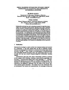
Figure 1.1: Example of how consistent phrases are extracted from a word alignment.

where the distortion model p(αk | αk−1 ) (the probability that the target segment k is aligned with the source segment αk ) is usually assumed to depend only on the previous alignment αk−1 (first order model).

1.3.2

Training phrase-based models

Ultimately, when learning a phrase-based model, the purpose is to compute a phrase translation table, in the form { xj . . . xj 0 , (yi . . . yi0 ) , p(xj . . . xj 0 |yi . . . yi0 )} where the first term represents a phrase from the source language, the second term represents a phrase from the target language, and the last term is the probability assigned by the model to the given bilingual phrase pair. In the last years, a wide variety of techniques to produce phrase-based models have been explored and implemented [23]. Firstly, a direct learning of the parameters of the equation p(˜ x|˜ y ) was proposed [48, 27]. Other approaches have been suggested, exploring more linguistically motivated techniques [41, 50]. However, the technique that has been more widely adopted is the one developed by [53], in which all phrase pairs coherent with a given word alignment are extracted. Since these word alignments are very restrictive because each target word is assigned only zero or one source words, sourceto-target and target-to-source alignments are combined heuristically. This procedure is

10


often called symmetrisation. Once this is done, the set of phrases consistent with the symmetrised word alignments is extracted from every sentence pair in the training set. An illustration of how this is done can be seen in figure 1.1 Most typically, the different features that are included into the translation model are: • Inverse translation probabilities, given by the formula p(˜ y |˜ x) =

C(˜ x, y˜) C(˜ x)

(1.8)

where C(˜ x, y˜) is the number of times segments x ˜ and y˜ were extracted throughout the whole corpus, and C(˜ x) is the count for phrase x ˜. • Direct translation probability, p(˜ x|˜ y ), which is obtained analogously. • Inverse and direct lexicalized features, which attempt to account for the lexical soundness of each phrase pair, estimating how well each of the words in one language translates to each of the words in the other language. These lexicalized features were defined in [53] • A constant feature, or phrase penalty, whose purpose is to avoid the use of many small phrases in decoding time, and favour the use of longer ones.

1.3.3

Tuning log-linear models

Log-linear models usually consists in a linear combination of log-models, also called feature functions. The score that a hypothesis receives when an input is presented to the system is the combination of the scores assigned by each of the models. But not every model has the same importance on the overall decision and their influence has to be gauged. For this reason, scaling factors adjust the discriminative power of every model participating in the log-linear combination. These scaling factors are typically learnt using a small amount of bilingual sentences, called a “development set”, since the amount of parameters whose value needs to be learnt is small, typically 14. The purpose is to select the best configuration of those scaling factors so that an error is minimised on the development set. This technique is called minimum error training (MERT)[32]. The most common tuning step when setting up a SMT system consists in translating the source part of the development set and also producing a set of N-best hypotheses for the translation of every sentence. Then, by using an optimisation algorithm like Powell’s algorithm [37], values for the scaling factors are estimated so that the best hypotheses within the computed N-Best lists score higher and are pushed up in the list. Immediately afterwards, a new translation of the source part of the development set is performed with the new scaling factors. This operation is repeated a certain amount of times or until a certain convergence has been achieved.

1.4. COMPUTER ASSISTED TRANSLATION

1.3.4

11

Decoding in phrase-based models

In the previous sections we have seen how to estimate the parameters involved in the translation process during the training and the tuning stages. This complex process is performed when setting up a statistical machine translation system and may take hours or days. Once a SMT system has been trained, it is time to do the actual work the system has been designed for: translate sentences from a source language into sentences of a target language. This process is called “decoding” and a decoding algorithm is needed for that purpose. Different search strategies have been suggested to define the way in which the search space is organised. Some authors [33, 18] have proposed the use of an A? algorithm, which adopts a best-first strategy that uses a stack (priority-queue) in order to organise the search space, and this strategy has become the most commonly used. On the other hand, a depth-first strategy was also suggested in [2], using a set of stacks to perform the search.

1.4

Computer assisted translation

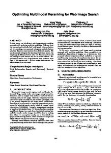
Translations provided by state-of-the-art SMT systems are still far from being reliable (or even understandable). In situations where only a shallow and very general understanding is required, SMT systems may provide an acceptable result. But in many other tasks, collaboration of a human translator is essential to ensure high quality results. Nowadays, machines are widely used by professional human translators to perform the task of translation. Then, a human-machine interaction becomes necessary and different instances of this interaction give form to the multiple available methods in the market of Computer assisted translation (CAT). Many long-experienced professional human translators would probably say that one of the best technological advances in the field of computer assisted translation was the introduction of word processors a couple of decades ago. Thus, professionals could draft and correct repeatedly a translation. Such a thing would have been almost impossible with a mechanical typewriter. Digital dictionaries can also be considered one of the first and more rudimentary elements of computer assisted translation. A natural extension to dictionaries are the socalled translation memories (TM). When a source phrase has been translated into a target phrase, the bilingual pair can be stored in a database to be used if it appears again. A collaborative database where multiple human translators add their phrases is a common and widely appreciated tool in CAT. Computer scientists strongly believe that computers have to play a more important role in the translation process to increase productivity. A simple way of introducing a machine to actively participate in the translation task is at the beginning of a sequential process [5] so that a SMT system produces a tentative translation that the professional human translator will accept or amend (fig. 1.2).

12


Figure 1.2: Scheme of a post-edition paradigm.

The satisfaction of human translators with this system highly depends on its performance. If the SMT system outputs sentences that only need small changes to be acceptable, then users will feel that their productivity has been increased and will favour the establishment of this technology. However, if the effort of correcting the hypothesis from the SMT system is equal or higher than the effort to translate the sentence from scratch, professional human translators will not be positive with the introduction of this paradigm. A refinement of this post-edition system would consist in measuring the degree of confidence that the SMT system has on its own hypotheses, and output them for the user to correct if and only if the confidence is above a certain threshold. A more sophisticated way to introduce the machine into the translation process is following the interactive machine translation (IMT) paradigm [1, 7]. In this paradigm, the SMT system proposes a hypothesis to the human translator who may accept the whole hypothesis as a final sentence. In the case of European languages, humans read from left to right. In this direction, when the user finds a mistake in the system’s hypothesis, the user clicks to place the cursor in the appropriate place to correct the mistake. In this moment, the system assumes that the user has validated the prefix up to the mistake, and then proposes a new suffix using the information from the click or from user’s keystrokes. In this master thesis, we assume the post-edition scenario due to its simplicity and will perform adaptation in a sentence by sentence basis.

1.5

Adaptation

Whenever the text to be translated belongs to a different domain than the training or development corpora, translation quality diminishes significantly [6]. For this reason, the adaptation problem is very common in SMT, where the objective is to improve the performance of systems trained and tuned on out-of-domain data by using very limited amounts of in-domain data or under other constraints on the amount of available data or time limitations. An effective approach for adaptation is filtering [28], where training sentences are explored in the search of finding data similar enough to the domain we are interested in. Then, such bilingual sentences can be used to increase the size of the tuning set, or to create other models on the new in-domain data and finally interpolate them with the out-of-domain data. Similarly, a resampling can be used on the set of training sentences

1.5. ADAPTATION

13

to weight their relevance to the in-domain task [44, 45]. Although these approaches are very interesting, they can only be used in batch adaptation as far as we know. A popular approach is to adjust either the feature functions or the log-linear weights, where the objective is to improve performance of systems by “shifting” their probability estimations. The principle of locality can be exploited to adjust scores or probabilities by using caches. In this approach, models trained on out-of-domain data can be interpolated with models trained on the last Q sentences that have been processed [10, 30, 26] and the performance in SMT has been carefully assessed in [47]. Other authors [24, 3] studied different ways to combine bilingual or only source data from different domains. The use of clustering to extract sub-domains to build more specific language or translation models has also been studied in [54, 43]. In [9], alignment model mixtures were explored as a way of performing topic-specific adaptation. Adapting a system to changing tasks is specially interesting in the computer assisted translation (CAT) and interactive machine translation (IMT) paradigms, and this is the problem that we address along this master thesis. In these paradigms, a SMT system proposes a hypothesis to a human translator, who may amend the hypothesis to obtain an acceptable target sentence and after that expects the system to learn dynamically from its own errors, so that the errors the human translator has corrected once do not have to be corrected over and over again. The approach for adaptation that has been imported from traditional SMT to CAT or IMT is based on batch learning. In batch adaptation for CAT and IMT, the learning process is performed with a set of translations that a user has produced from a set of input sentences from a source language, with the aid of a suitable machine translation system (fig.1.2). Such a set of translations, together with their corresponding input sentences form a bilingual set that is used to optimise some parameters involved in the translation process. In traditional SMT, such parameter optimisation requires a certain amount of computational resources and a considerable amount of time. But it does not pose any problem since all the process is performed off-line before the actual translation task takes place. In that sense, CAT and IMT are very different paradigms from the adaptation point of view. Those systems work under the constraint of user interaction and, for real tasks, the nature of the source text to be translated might constantly vary in an unpredictable way. For this reason, batch adaptation is not appropriate to cope with both problems since it forces us to perform a costly optimisation after translating a certain number of sentences. The challenge is then to make the best use of every correction provided by the user by adapting the models in an online manner, i.e. without the need of a complete retraining of the model parameters, since such retraining would be too costly. Different approaches to cope with online adaptation have been proposed so far in a

14


sentence-by-sentence basis. In [34], an online learning application is presented for IMT, where the models involved in the translation process are incrementally updated by means of an incremental version of the expectation-maximisation algorithm via sufficient statistics, allowing for the inclusion of new phrase pairs into the system. The intention of our work is not the inclusion of new phrase pairs into the system, but to adapt the prediction mechanisms. The technique proposed here can be applied to any search strategy, since it only relies on a dynamic reranking algorithm which is applied to a N-best list, regardless of its origin. This allows us to compare several different online learning strategies in any system that is able to produce a set of hypotheses for every input sentence. The authors in [14] use the perceptron algorithm to obtain more robust estimations of the scaling factors (λ) by iterating several times (epochs) on a development set until a desired convergence is achieved. In section 2.2.2, a similar strategy is followed, although in the present work we apply it for learning λ and h in an online manner instead of batch. That is, we will work under the implicit constraint of online scenarios, where every observation cannot be processed an indefinite number of times. In [39] the authors propose the use of the passive-aggressive framework [12] to do an online updating of the feature functions h. They propose the integrated use of a memorybased MT system and a SMT system. In this setup, the SMT system is only triggered when the memory-based MT system is unable to produce a satisfactory translation. In both cases, the combined system is fed back with the final translation produced by the user. Then, the memory-based MT system includes it into the translation memory, and the SMT system activates an online learning procedure. For this reason, the performance of their online learner is only evaluated on a small subset of the original sentences to be translated. Improvements obtained were very limited, since adapting h is a very sparse problem and the subset of sentences used to do online adaptation was small. In this work, in order to objectively observe the behaviour of the online learner, the translation memory was removed from the interaction cycle so that the SMT system always proposes a target sentence to the user. Different heuristic variations of the passive-aggressive (PA) framework were also analysed and the passive-aggressive framework was applied to adapt either the translation features or the scaling factors. In this work, several online learning techniques are proposed, in which the purpose is to use the information from the last user interaction to hopefully improve the quality of subsequent translations. Two alternatives for incorporating the feedback provided by the user are presented. On the one hand, different strategies for adapting λ, and on the other hand, alternatives for acting directly on the feature functions h of eq. (1.5). The intention is to compare the adequacy of either adapting the feature functions and the loglinear weights λ, which is shown in [42] to be a good adaptation strategy. In [42], the authors propose the use of a Bayesian learning technique in order to adapt the scaling factors based on an adaptation set. In contrast, in the present work, the purpose is to perform online adaptation, i.e. to adapt the system parameters after each new sample has been provided to the system.

1.6. CONCLUSIONS

1.6

15

Conclusions

Machine translation has been a topic of interest since the very first computer was conceived. Within the wide range of historical approaches, statistical machine translation seems to be the most promising system in combination with phrase-based models. It has been shown how training, tuning and decoding are performed nowadays and the difficulties derived from a system when facing a task it has not been trained for. Thus, adaptation is one of the topics that researchers are concerned about, specially when machine translation systems have a continuous interaction with human translators and need to be constantly adapted. The contributions of this thesis are as follows. First, a new application of the perceptron algorithm for online learning in SMT is proposed. Second, the passive-aggressive framework for scaling factor adaptation is applied and compared to previous work. Third, a new discriminative technique is proposed for incrementally learning the scaling factors λ and the feature functions h, which relies on the concept of Ridge regression, and which proves to perform better than the perceptron and the passive-aggressive algorithms for scaling factor adaptation in all analysed language pairs. Finally, a sound exhaustive comparison of strategies and methods for every approach is provided. Although applied here to phrase-based SMT, both strategies can be applied to rerank a N-best list, which implies that they do not depend on a specific training algorithm or a particular SMT system. Along this thesis, a formalisation of the problem of online learning in a post-editing scenario is developed in chapter 2. In section 2.1, two approaches for incorporating the feedback provided by the user into the models are described, and then several online learning techniques in section 2.2 are analysed and others are proposed, in which the purpose is to use such information to hopefully improve the quality of subsequent translations. In chapter 3, the experimental environment is described in detail and traditional and our proposed techniques are evaluated when applied to both approaches. A study on metric correlation in reranking is provided in chapter 4.2. Finally, conclusions and future work can be found in chapter 5.

Chapter 2

Online learning in CAT

Adaptation in IMT or the post-edition strategy in the CAT paradigm is usually required to be performed progressively, as the user (i.e. human translator) interacts with the system. But traditional algorithms for tuning using minimum error rate training (MERT) procedure are used in batch mode. That is, the algorithms are fed with the whole tuning sets and observations are processed as many times as necessary. However, in a real CAT or IMT task, it is not realistic to process all previous observations after every interaction with the user, since it is computationally expensive and very time demanding. In general, in an online learning framework, the learning algorithm processes observations sequentially and then, they are not reviewed anymore. After every input, the system makes a prediction and then receives a feedback. The information provided by this feedback can range from a simple opinion of how good the system’s prediction was, to the true label of the input in completely supervised environments.

Figure 2.1: Scheme of the post-edition technique within the computer assisted translation paradigm incorporating feedback from a professional human translator in an on-line manner.

In this work, user’s feedback is incorporated into the system by means of an artificially created rerank module. The SMT system will provide a list of the best hypotheses instead of the single best hypotheses. The goal of the rerank module is then to select the 17

18

CHAPTER 2. ONLINE LEARNING IN CAT

best hypothesis within the N-best list. Note that such hypothesis is not necessarily the first one appearing on the top of the list. The purpose of online learning algorithms is to modify the selection mechanisms of the rerank module in order to improve the quality of future selections. Specifically, in a CAT scenario, the SMT system receives a sentence in a source language and then outputs a sentence in a target language as a prediction based on its models. The user, typically a professional human translator, post-edits the system’s hypothesis thus producing a reference translation yτ . Such a reference can be used as a supervised feedback (fig.2.1). Our intention is to learn from that interaction. Then, eq. (1.5) is redefined as follows ˆ t = argmax y yt

M X

λtm htm (xt , yt )

(2.1)

m=1

That is, in vectorial form: ˆ t = argmax λt ht (xt , yt ) y

(2.2)

yt

where both the feature functions ht and the log-linear weights λt vary according to the samples (x1 , y1 ), . . . , (xt−1 , yt−1 ) seen before time t. In order to simplify notation, we will omit the subindex t from the input sentence y and output sentence x, although such subindex is always assumed. We can either apply online learning techniques to adapt ht , or λt , or both at the same time. In this work, however, we will not try to adapt both at the same time. To unclutter notation, let y be the hypothesis proposed by the system (ˆ y so far), and y∗ the best hypothesis the system is able to produce in terms of translation quality (i.e. the most similar sentence with respect to yτ ). Ideally, we would like to adapt the model parameters (be it λ or h) so that y∗ is rewarded, that is, achieves a higher score according to the models within eq. (1.5). We define the difference in translation quality between the proposed hypothesis y and the best hypothesis y∗ in terms of a given quality measure µ(·): l(y) = |µ(yτ , y) − µ(yτ , y∗ )|,

(2.3)

where the absolute value has been introduced in order to preserve generality, since in SMT some of the quality measures used, such as TER [46], represent an error rate (i.e. the lower the better), whereas others such as BLEU [36] measure precision (i.e. the higher the better). In addition, the difference in probability between y and y∗ is proportional to φ(y) = s(x, y∗ ) − s(x, y). (2.4) Ideally, we would like that increases or decreases in l(·) correspond to increases or decreases in φ(·), respectively: if a candidate hypothesis y has a translation quality µ(y) which is very similar to the translation quality provided by µ(y∗ ), we would like that such fact is reflected in the translation score s, i.e. s(x, y) is very similar to s(x, y∗ ). Hence, the purpose of our online procedure should be to promote such correspondence after processing sample t.

19

2.1. APPROACHES

2.1

Approaches

In the following two subsections, we analyse two approaches for online adaptation. Those approaches consist in either adapting the feature functions h or adapting the scaling factors λ from the log-linear model. Those two tasks have different interesting properties. The former allows us to fine-tune parameters at the phrase level and intuitively makes us think that we have a higher control on the adaptation task. However, this task is very sparse and the proposed online algorithms will have different levels of success. Scaling factor adaptation consists in a rough tuning of the discriminative power of every feature function and usually implies the estimation of a reduced number of parameters. A formalisation of the problems will be introduced, and the methods to cope with them will be presented in section 2.2.

2.1.1

Adapting feature functions

There have been proposed a number of feature functions that somehow describe different aspects of statistical machine translation systems. Some of these models are more or less effective than others and they are included in the log-linear combination of eq. (1.5) if they lead to statistically significant improvements over the base system. As described in section 1.3, state-of-the-art phrase-based translation systems use phrases as their main building blocks to infer translations and there is a subset of feature functions, called translation models, that are defined locally on bilingual phrases. That is, each translation model assigns a score to every phrase that has been extracted from the training corpus. Commonly, they are the direct and inverse lexical probability models, direct and inverse phrase probability models and a word insertion penalty model. From now on, when stating that we are going to adapt feature functions, we will refer to adapt specifically the feature functions related to the translation models. Although there might be some reasons for adapting all the score functions h, in the present work we focus on analysing the effect of adapting only the feature functions related to the translation models. For this purpose, we need to define hs (x, y) as the combination of the n translation models implicit in current translation systems. Since those models are typically specified at phrase level (˜ xk , y˜k ) for k = 1, . . . , K where K is the number of phrases conforming the sentence pair (x, y), hs (x, y) can then be defined as: hs (x, y) =

X n

λn

X

hn (˜ xk , y˜k )

(2.5)

k

where hs can be considered as a single feature function h in eq. (1.5) describing a sentence pair (x, y). Then, we can study the effect of adapting the translation models in an online manner by adapting hs . By introducing a weight parameter ut−1 (˜ xk , y˜k ) for every phrase score

20


hn (˜ xk , y˜k ) of equation 2.5, an auxiliary function ut−1 (x, y) can be defined such that X X λn ut−1 (˜ xk , y˜k )hn (˜ xk , y˜k ) hts (x, y) = n

=

X

k

ut−1 (˜ xk , y˜k )

k

X

λn hn (˜ xk , y˜k )

n

= ut−1 (x, y)hs (x, y),

(2.6)

and considering all the models hm (·, ·) that are not part of hs , that is, ∀m = 6 s : t hm (·, ·) = hm (·, ·), the decision rule in eq. (2.1) is approximated as X ˆ t = argmax y λm hm (x, y) + hts (x, y). (2.7) y

m6=s

A general expression for the update step of the online learning algorithms presented in this chapter to adapt the translation models is then easily defined as: ut (x, y) = ut−1 (x, y) + αν t

(2.8)

where ut−1 (x, y) is the update function that has been learnt after observing the previous (x1 , y1 ), . . . , (xt−1 , yt−1 ) pairs and α is the learning rate. In eq. (2.6), we observe the inner product of two terms. If the phrase-table contains p bilingual entries, hs (x, y) is a column vector of p rows assigning a score to every bilingual phrase. The value of every entry is nothing else than the recombination of the traditional scores appearing on the phrase-table with their corresponding weights of the log-linear model. Then, every hypothesis can be represented by a column vector of p real numbers where the value of the i-th component is the score of the i-th phrase-table entry if such an entry was used to build that hypothesis. The rest of elements of the column vector which represents the hypothesis are null. With this consideration, hs (x, y) ∈ Rp is the column vector of real numbers that represent a translation y of a source sentence x. In practise, the phrase-table contains thousands or millions of entries, but only a few of them are used to build a sentence. For this reason, we consider this a very sparse problem with the common difficulties associated to this fact. Note that if we set to one every component of ut−1 (x, y), the result of the inner product ut−1 (x, y)hs (x, y) plus the score of other models different to the translation one is equivalent to the score of the hypothesis y given by a traditional SMT system.

2.1.2

Adapting scaling factors

A coarse-grained technique for tackling with the online learning problem in SMT implies adapting the log-linear weights λ (also called scaling factors). With this idea in mind, after the system has received the sentence ytτ as correct reference for an input sentence ˆ t corresponding to the sentence xt , our purpose is to compute the best weight vector λ pair observed at time t.

2.2. METHODS

21

The purpose is that the discriminative power of every model is adjusted such that the score resulting from the log-linear combination is higher for the most similar hypothesis ˆ t has been computed, λ yt∗ to ytτ than the score of any other hypothesis. Then, once λ can be updated as: ˆt λ = λt−1 + αλ (2.9) for a certain learning rate α. ˆ t is more general The information that is usually taken into account to compute λ and imprecise than the information used in adapting feature functions, but the variation in the score of eq. (1.5) can be higher since we will be modifying the scaling factors of the log-linear model. That is, when adapting the system to a different domain, we are going to adjust the importance of every single model to a new task in an online manner. In this approach, the usual number of parameters that are to be estimated equals to the number of models participating in the log-linear combination (which is small), as opposed to the huge number of parameters that feature function adaptation requires.

2.2

Methods

When a given input sentence x is presented to the SMT system, it produces a N-best list of hypotheses that are translations of x into the target language. Most of those hypotheses will not be as good as the one selected by the baseline system and that has maximum score, but there will be other hypotheses that will be indeed better in terms of a given quality metric. A good predictor should be able to find the best hypotheses within the N-best list that are better than the baseline in order to provide them as a final output. As described in section 2.1, in online learning algorithms, an update step is necessary to adjust the prediction mechanisms in the reranking module. In such update steps, some parameter values are “shifted” towards a more desirable value configuration with a certain step-size α. In our methods, we focus on how this update should be performed to compute ν t in ˆ t in eq. (2.9). eq. (2.8) or to compute λ There are several methods that can be used to compute the update step. In the following subsections, we describe the philosophy they follow, provide formalised solutions and show how they can be applied in our task.

2.2.1

Passive-aggressive

Online passive-aggressive (PA) algorithms [12] are a family of margin-based online learning algorithms that are specially suitable for adaptation tasks where a convenient change in the value of the parameters of our models is desired after every sample is presented to the system. Passive-aggressive algorithms are based on the concept of “margin”. It uses the margin (distance of the instance to the hyperplane) to modify the current classifier. The

22


general idea is to learn a weight vector representing a hyperplane such that differences in quality also correspond to differences in the margin of the instances to the hyperplane. The update is performed in a characteristic way in which we wish to achieve at least a unit margin on the most recent example but we also want to remain as close as possible to the current hyperplane. In this case, passive-aggressive algorithm is applied to a regression problem, where target value µ ˆ(y)t ∈ R has to be predicted by the system for input observation xt ∈ Rn at time t by using a linear regression function µ ˆ(y)t = wt · xt . After every prediction, the true target value µ(y)t ∈ R is received and the system suffers an instantaneous loss according to a sensitivity parameter : ( 0 if |w · x − µ(y)| ≤ l (w; (x, µ(y))) = (2.10) |w · x − µ(y)| − otherwise If the system’s error falls below , the loss suffered by the system is zero and the algorithm remains passive, that is, wt+1 = wt . Otherwise, the loss grows linearly with the error |ˆ µ(y) − µ(y)| and the algorithm aggressively forces an update of the parameters. The idea behind the passive-aggressive algorithm is to modify the parameter values of the regression function so that it achieves a zero loss function on the current observation xt , while remaining as close as possible to the previous weight vector wt . That is, formulated as an optimisation problem subject to a constraint [12]: 1 wt+1 = argmin ||w − wt ||2 + Cξ 2 n w∈R 2

s.t. l (w; (x, µ(y))) = 0

(2.11)

where ξ 2 is, according to the so-called passive-aggressive type-II, a squared slack variable scaled by the aggressivity factor C. As in classification tasks, it is common to add a slack variable into the optimisation problem to get more flexibility during the learning process. It is only left to create an auxiliary Lagrangian function from eq.(2.11), add the constraint together with a Lagrangian variable and set the partial derivatives to zero to obtain the closed form of the update term. As described in [39], passive-aggressive can be used for adapting the translation scores within state-of-the-art translation models. The optimisation problem in feature function adaptation is then 1 2 2 ||u(x, y) − ut−1 (x, y)|| + Cξ min (2.12) u,ξ>0 2 subject to constraint u(x, y)Φt (y) ≥

p l(y) − ξ,

(2.13)

where ξ is a slack variable, and Φt (y) is a column vector such that Φt (y) = [φ(˜ y1 ), . . . , φ(˜ yK )]0 ≈ hs (x, y∗ ) − hs (x, y)

(2.14)

23

2.2. METHODS

since all the rest of score functions except hs remain constant and the only feature functions we intend to adapt are the ones in hs . The solution to the optimisation problem in (2.12) has the form p lt (y) − ut−1 (x, y)Φt (y) (2.15) ν t = Φt (y) ||Φt (y)||2 + C1 in the passive-aggresive algorithm type II [39], where the parameter C is the aggressiveness of the algorithm. Similarly, to adapt the scaling factors λ: p ˆ t = Φt (y) lt (y) − λt−1 Φt (y) λ (2.16) ||Φt (y)||2 + C1 is used, where Φt (y) = [φ1 (y), . . . , φM (y)]0 = h(x, y∗ ) − h(x, y),

(2.17)

that is, all feature functions are taken into account. In [39], the update is triggered only when the proposed hypothesis violates the constraint p ut−1 (x, y)Φt (y) ≥ lt (y) (2.18) or, alternatively for the scaling factors adaptation: p λt−1 Φt (y) ≥ lt (y)

(2.19)

Heuristic variations Several update conditions different to eq. (2.18) or to eq. (2.19) have been explored in this work. The most obvious is to think that an update has to be performed every time that the quality of a predicted hypothesis y is lower than the best possible hypothesis yt∗ in terms of a given quality measure µ. That is, when the following condition holds: ∃y∗ : |µ(yt , y∗ ) − µ(yt , y)| > 0

(2.20)

where y∗ is used for the update step. The idea behind this heuristic is to reward those phrases that appear in y∗ but did not appear in y, and symmetrically, to penalise phrases that appeared in y but not in y∗ . However, it can be often observed that there are several distinct hypotheses y0 whose quality is as high as the quality of y∗ . Hence, it can also be interesting to use these hypotheses for the update step. Thus, in the second heuristic we are interested in considering all those sentences y0 such that ∀y0 : µ(yt , y0 ) = µ(yt , y∗ ).

(2.21)

Lastly, it might also be desirable to reward phrases appearing in hypotheses y0 whose quality is not as high as the quality of y∗ , but still are better than the proposed hypothesis

24


by the system (and penalise phrases from y that do not appear in any y0 ). The formalisation of this extension to conditions (2.18) and (2.19) is to perform the update for every hypothesis y0 that is better than the one proposed by the system in terms of our quality measure: ∀y0 : l(y0 ) < l(y) (2.22) they are, all those hypotheses y0 such as the difference in quality with respect to the reference y∗ is smaller than the difference in quality of the system’s proposed hypothesis y with respect to y∗ .

2.2.2

Perceptron

The perceptron algorithm [40, 11] is an error driven algorithm that estimates the weights of a linear combination of features by comparing the output y of the system with respect to the true label yτ of the corresponding input x. The perceptron iterates through the set of samples a certain number of times (epochs), or until a desired convergence is achieved. The implementation in this work follows the proposed application of a perceptronlike algorithm in [14]. However, for comparison reasons in our online adaptation for the CAT framework, the perceptron algorithm will not visit a sample again after being processed once. A standard single-layer perceptron has a number of inputs whose dimensionality depends on the dimension of the observations. Every variable of a given observation is weighted and then linearly combined with the rest of the variables to produce a single output. As an error-driven algorithm, the output produced by the perceptron is compared to the ideal target value and the parameters of the perceptron, namely the weights of the inputs, are adjusted to minimise the difference between the target and the output value. For feature function adaptation, input samples in the proposed perceptron are pdimensional feature vectors hs (x, y). Those feature vectors are combined linearly in the single layer of the perceptron with the weights from the auxiliary function ut−1 (x, y). Using the feature vector hs (x, y) of the system’s hypothesis y and the feature vector hs (x, y∗ ) of the best hypothesis y∗ from the N-best list, the update term ν t is computed as follows: ν t = sign(hs (x, y∗ ) − hs (x, y)) (2.23) In order to adapt the scaling factors, the necessary perceptron will be much smaller since the input samples h(x, y) are M -dimensional, where M is the total number of models (typically around 14). Those feature vectors are combined linearly in the single ˆ is computed as: layer of the perceptron with the scaling factors λ, and the update term λ ˆ t = sign(h(x, y∗ ) − h(x, y)) λ

(2.24)

The perceptron-like algorithm is, among the algorithms that are being studied in this work, the most simple and fast method to update parameters in an on-line manner since it only involves three floating point operations on vectors.

25

2.2. METHODS

Note that, in this perceptron-like algorithm, the sign operator forces the algorithm to make fixed-size steps in the adaptation of the parameters, which can be seen as a watereddown version of the standard and widely used perceptron whose steps are calibrated by the difference of the desired output and the actual output. The decision to use a perceptron-like algorithm instead of a real perceptron was made for comparison reasons, since the former method was successfully applied in a similar task[14].

2.2.3

Discriminative regression

It has been observed in previous methods that the update term is computed using the information extracted from the comparison of the hypothesis originally proposed by the system, and the best hypothesis from the N-best list according to a reference translation. As we saw, the perceptron and the passive-aggressive algorithms try to find a configuration in the values of the weight vectors (λ or u) such that good hypotheses within the N-best list tend to score higher. This effect is indeed desirable, but we would still add another property: we would also like that bad hypotheses score lower. In order to achieve such an ambitious objective, all hypotheses within the N-best list are going to be used by this algorithm, as opposed to the perceptron and the passiveaggressive algorithms that used only the best hypothesis within the N-best list. This method uses more information during the search of the best possible configuration of weight values, with the aim of finding one such that rewards good hypotheses and penalises bad ones. For simplicity, let’s first study the application of this method on scaling factor adaptation and then, we will see how it works for feature function adaptation. ˆ t such that increments in s(x, y) correspond to improveThe problem of finding λ ments in the translation quality metric µ(y) as previously described in the introduction ˆ t such that the difference in scores φ(y) of of this chapter, can be viewed as finding λ two given hypotheses approximate their difference in translation quality l(y). So as to formalise this idea, let us first define some matrices for the case of scaling factors adaptation, since it is the most simple scenario. Let N-best be the list of N best hypotheses computed by our system for sentence x. Let be a matrix Hx of size N × M , where M is the number of features in eq. (1.5), containing the feature functions h of every hypothesis of the N-best list produced for an input sentence x, defined such that sx = Hx · λt−1

(2.25)

where sx is a column vector of N entries with the log-linear score combination of every hypothesis in the N-best list. Additionally, let H∗x be a matrix with N rows such that   h(x, y∗ )   .. H∗x =  (2.26)  . h(x, y∗ )

26


where all rows are identical and equal to the features of hypothesis y∗ . Then, Rx can be defined as the difference between H∗x and Hx : Rx = H∗x − Hx

(2.27)

ˆ such that differences in scores are reflected as The key idea is to find a vector λ differences in the quality of the hypotheses. That is, ˆ t ∝ lx Rx · λ

(2.28)

where lx is a column vector of N rows such that lx = [l(y1 ) . . . l(yn ) . . . l(yN )]0 , ∀yn in the N-best list of x are the differences in quality of every hypothesis with respect to the best one. ˆ such that The objective is to find λ ˆ = argmin |Rx · λ − lx | λ

(2.29)

λ

= argmin ||Rx · λ − lx ||2

(2.30)

λ

where || · ||2 is the euclidean norm. Although eqs. (2.29) and (2.30) are equivalent (i.e. the λ that minimises the first one also minimises the second one), eq. (2.30) allows for a ˆ can be computed as direct implementation thanks to the Ridge regression1 , such that λ ˆ = lx , given by the equation: the solution of the overdetermined system Rx · λ ˆ = R0 · Rx + βI −1 R0 · lx λ x x

(2.31)

where a small β is used as a regularisation term to stabilise R0x · Rx and to ensure it has an inverse. In the case of feature function adaptation, there is a similar application of this method. Similarly, Hx contains the scores for every hypothesis from the N-best list: 

 hs (x, y1 )   .. Hx =   .

(2.32)

hs (x, yN ) and H∗x is simply defined as:  hs (x, y∗ )   .. H∗x =   . 

hs

(2.33)

(x, y∗ )

Finally, the expression to compute the update term is given by: ν t = R0x · Rx + βI 1

Also known as Tikhonov regularisation in statistics.

−1

R0x · lx

(2.34)

27

2.3. CONCLUSIONS

Note that, as a difference from eq. (2.25), the column vector representing the scores of every hypothesis from the N-best list, sx , is computed as: sx = Hmx · λm + Hx · ut−1

(2.35)

where Hmx is an N × (M − n) matrix containing the feature functions that are not present in the translation models, i.e. the language model or reordering models, for every hypothesis from the N-best list, and the scaling factors λm are the corresponding weights to the models in Hmx .

2.3

Conclusions

Although there are many possibilities to perform adaptation, in this chapter, it has been described how to perform online adaptation in an interactive scenario. There were mainly two strategies to adapt the system, namely feature function adaptation and scaling factor adaptation, each of them having different characteristics. Then, three algorithms to perform the adaptation in either strategy have been introduced. The passive-aggressive algorithm is an on-line learning algorithm that has been applied out-of-the-box, while the perceptron has been slightly modified to run in an online manner. Finally, a new online learning algorithm has been proposed, which rewards good hypotheses and penalises bad ones, with the hope to outperform all the algorithms that have been studied in section 2.2.

Chapter 3

Experiments

3.1

Experimental setup for online adaptation

Ideally, for experimentation purposes in a CAT scenario it would be required to involve a number of human translators to interact with our SMT systems. However, a true CAT scenario is very expensive for large experiments involving many languages, since it requires a human translator to correct every hypothesis produced. As an alternative to the use of human translators to post-edit the system’s hypotheses, we can simply use the target reference present in the test set and feed one sentence at a time, given that this would be the case in an online CAT process. As baseline system, we trained a SMT system on the Europarl training data, in the partition established in the workshop on SMT of the NAACL 20091 . Specifically, we trained our initial SMT system by using the training and development data provided that year. The Europarl corpus [21] is a parallel corpus that has been extensively used in statistical machine translation tasks, where the quality of the bilingual corpus is an important characteristic. The Europarl corpus is extracted from the proceedings of the European parliament published on the web and it includes 11 European languages. Statistics are provided in table 3.1. The open-source MT toolkit Moses [25]2 is a statistical machine translation system that performs the training of translation models of any language pair given a set of bilingual sentences. It also implements a decoding algorithm that allows to efficiently find the translation of an input sentence with the highest probability. This toolkit was used in its default setup, and the 14 weights of the log-linear combination were estimated using MERT [32] on the Europarl development set. Additionally, a 5-gram language model with interpolation and Kneser-Ney smoothing [19] was estimated. Since our purpose is to analyse the performance of different online learning strate1 2

http://www.statmt.org/wmt10/ Available from http://www.statmt.org/moses/

29

30

CHAPTER 3. EXPERIMENTS

Table 3.1: Characteristics of Europarl corpus. Devel. stands for development, OoV for “out of vocabulary” words, “Av.g sen. len” stands for the average sentence length, K for thousands of elements and M for millions of elements. Data statistics were collected after tokenising, lowercasing and filtering out long sentences (> 40 words). Es

Training

Devel.

Sentences Run. words Avg. sen. len Vocabulary Sentences Run. words Avg. sen. len OoV. words

En 1.3M 27.5M 26.6M 21.15 20.46 125.8K 82.6K 2000 60.6K 58.7K 30.3 29.35 164 99

Fr

En 1.2M 28.2M 25.6M 23.5 21.33 101.3K 81.0K 2000 67.3K 48.7K 33.65 24.35 99 104

De

En 1.3M 24.9M 26.2M 19.15 20.15 264.9K 82.4K 2000 55.1K 58.7K 27.55 29.35 348 103

Table 3.2: Characteristics of News Commentary test sets. OoV stands for “out of vocabulary” words with respect to the Europarl training set. Data statistics were collected after tokenising and lowercasing. Es Test 08

Test 09

Sentences Run. words Avg. sen. len OoV. words Sentences Run. words Avg. sen. len OoV. words

En

2051 52.6K 49.9K 25.64 24.33 1029 958 2525 68.1K 65.6K 26.97 25.98 1358 1229

Fr

En

2051 55.4K 49.9K 27.01 24.33 998 963 2525 72.7K 65.6K 28.79 25.98 1449 1247

De

En

2051 55.4K 49.9K 27.01 24.33 2016 965 2525 62.7K 65.6K 24.83 25.98 2410 1247

gies, in addition to Europarl we also considered the use of two different News-Commentary (NC) test sets, from the 2008 and 2009 ACL shared tasks on SMT. The News-Commentary corpus consists in a set of pieces of news that have a specific domain different to the proceedings of the European parliament speeches. Since this corpus comes from a different source it is widely used to test system’s performance in the adaptation task. Statistics of these test sets can be seen in table 3.2. Note that those test sets correspond to sentences from a different domain than the one in the Europarl corpus, having different linguistic characteristics like grammar structure or sentence length. Experiments were performed on the English → Spanish, English → German and English → French language directions for NC test sets of 2008 and 2009. For sections 2.2.1 and 2.2.2, the true best hypothesis yτ is impossible to compute because we would need to examine the exponential number of hypotheses that a SMT system is able to produce. However, a bigger and more decisive problem is the lack of

3.1. EXPERIMENTAL SETUP FOR ONLINE ADAPTATION

31

coverage of the models. For these reasons, instead of using the true best hypothesis, the best hypothesis within a given N-best list was selected. In the experimentation section of every approach, there are two sets of experiments. The first one is carried out to evidence the performance of the online learning algorithms in a sentence-by-sentence basis. In those experiments, the size of the N-best list is fixed to N = 1000 hypotheses. This size influences on two aspects: 1. The selection of the best hypothesis y∗ . If the size of the list is smaller than N = 1000, let’s say N = 500, the best hypothesis y∗ with respect to a reference yτ may not be the same any more because y∗ may have not appeared within the first 500 hypotheses. Thus, the quality of y∗ from the smaller 500-list will be less or equal than y∗ from the 1000-list. 2. The prediction task becomes more difficult as the size of the list of possible candidates increases. We have observed that most of the hypotheses from the N-best list are worse than the one originally proposed by the system. Moreover, SMT systems produce their N-best lists in descending order of log-combined score. Such a fact means that when the size of the N-best list is big, the potential number of hypotheses with lower quality is also big and the number of bad hypotheses with respect to the good ones increases. Thus, the second set of experiments focuses on testing different sizes of the N-best list and observing its impact on the overall quality score. Although the final BLEU and TER scores are reported for the whole considered test set, all of the experiments described there were performed following an online CAT approach: each reference sentence was used for adapting the system parameters after such sentence has been translated and its translation quality has been assessed. For this reason, the final reported translation score corresponds to the average over the complete test set, even though the system was still not adapted at all for the first samples. There is a number of free parameters in the algorithms that have been described in section 2.2 and they have been all adjusted according to preliminary investigation on a disjoint development set, as follows: • Section 2.2.1: C → ∞ ( C1 = 0 was used) in both approaches. • Section 2.2.2: α = 0.001 for λ-adaptation and α = 0.050 for h-adaptation. • Section 2.2.3: α = 0.005 for λ-adaptation and α = 0.001 for h-adaptation, both with a regularisation term β = 0.01. The abbreviations on the plots shown in the following sections are as follows: • PA is the passive-aggressive technique described in section 2.2.1, with the update trigger described in eq. (2.18).

32


• PA var. is the same technique as above, but applying the variation described in eq. (2.20).

• percep. stands for the perceptron-like technique described in section 2.2.2, and

• Ridge for the discriminative Ridge regression described in section 2.2.3.

3.1.1

Quality metrics

Translation quality will be assessed by means of the BLEU [36] and TER [46] scores. BLEU (bilingual evaluation understudy) was one of the first methods to achieve a high correlation with human judgement and remains one of the most popular metrics to evaluate how good a machine-translated text is with respect to a certain reference. It is a precision metric that measures n-gram precision implementing a geometrical average with a penalty for sentences that are too short. A metric from a different nature is TER (translation error rate). It is an error metric that computes the minimum number of edits required to modify the system hypotheses so that they match the references. Possible edits include insertion, deletion, substitution of single words and shifts of word sequences. This error metric has been reported to also correlate well with human judgement and will be extensively used to assess quality in our experiments. Hence, for computing y∗ as described in section 2, either BLEU or TER will be used, depending on the reported evaluation measure (i.e. when reporting TER, TER will be used for computing y∗ ). One consideration that we have to point out at this stage is that BLEU is commonly used at a document level showing a high correlation with human judgement, but it is not well-defined at sentence level and may often be zero for all hypotheses, which means that y∗ is not always well defined and it may not be possible to compute it. An easy example to observe this behaviour is the translation of the English sentence “This is red” with a reference Spanish sentence “Esto es rojo”. Even if the system is able to perfectly match the reference translation, the BLEU score will be zero since the number of 4-grams in common with the reference will be zero. For this reason, such samples will not be considered within the online procedure. Another consideration is that BLEU and TER might not be correlated, i.e. improvements in TER do not necessarily mean improvements in BLEU. This is analysed more in detail in section 4.2. Statistical significance of the improvements over baseline scores are calculated using the bootstrapping resampling technique with 10.000 repetitions with replacement. By using this technique, it is possible to compute the confidence intervals and pair-wise improvement interval to test the significance of the results obtained by the studied algorithms. Further details of this bootstrapping technique can be found in [20].

3.2. EXPERIMENTAL RESULTS FOR ONLINE ADAPTATION

3.2

33

Experimental results for online adaptation

One of the main objectives of this master thesis is the exhaustive evaluation of the performance of the online learning algorithms presented in section 2.2 applied to the approaches studied in section 2.1. For this reason, we will carefully assess in section 3.2.1 the behaviour of the passiveaggressive, perceptron and discriminative regression algorithms to the task of adapting feature functions (h) related to the translation models. A similar evaluation will be carried out for scaling factor (λ) adaptation in section 3.2.2. Some algorithms are expected to perform better in one task than in the other. To put all together, a final comparison among the algorithms applied to the tasks where they perform better will be shown in order to extract conclusions about the convenience of the use of certain algorithms to cope with the online learning in every approach. As a baseline for our experiments, we will use a system that does not perform adaptation or, in other words, a trivial algorithm implemented in the rerank module that always selects the first hypothesis proposed by the SMT system. From a list of N-best hypotheses obtained by traditional methods from the SMT system, the algorithms from section 2.2 implemented in the rerank module will predict the difference in quality of every hypothesis with respect to the best hypothesis (which is still unknown). Then, the rerank module will sort the hypotheses in descending order by their predicted quality and the hypothesis resulting on the top of the sorted list will be provided as an output.

3.2.1

Adapting feature functions

Different aspects of the behaviour of the online learning algorithms from section 2.2 when applied to feature function adaptation are to be studied. In the first set of experiments of this section, the improvement of the online learning algorithms over the baseline system is evaluated. Specifically, in the plots shown in fig. 3.1, the translation pair was English → French, the test set was the NC 2009 test set, and the size of the considered N-best list was 1000. The two plots on the left display the average BLEU and TER scores up to the t-th sentence. That is, the BLEU/TER score at the t-th sentence can be interpreted as the traditional BLEU/TER score if the test set had t sentences in total. The reason for plotting the average BLEU/TER is that plotting individual sentence BLEU and TER scores would result in a very chaotic, unreadable plot; in fact, such chaotic behaviour can still be seen in the first 100 sentences. The two plots on the right display average BLEU and TER improvements with respect to the baseline translation quality. In other words, they display at sentence t the improvements of the different algorithms if the test set had t sentences. Although apparently irrelevant to the performance of the online learning algorithms, the two plots on the left in fig. 3.1 have a unique characteristic shape for that language pair and that test set. It can be seen that BLEU and TER improve after 1500 sentences have been presented to the system. The only explanation to this shape is that after the

34


1500-th sentence, there are around 300 sentences that are easier to translate and that increases (or decreases) the average of the BLEU (or TER). BLEU evolution baseline PA PA var. percep. Ridge

23 22 BLEU

21 20 19

1

0.5 BLEU difference

24

BLEU Learning curves

0

-0.5

18

baseline PA PA var. percep. Ridge

-1

17 16 0

500

1000 1500 Sentences

2000

2500

0

500

TER evolution

67 TER

2500

2.5 2 TER difference

68

2000

TER Learning curves baseline PA PA var. percep. Ridge

69

1000 1500 Sentences

66 65


1.5 1 0.5

64 0

63 0

500

1000 1500 Sentences

2000

2500

0

500

1000 1500 Sentences

2000

2500

Figure 3.1: BLEU/TER evolution and learning curves for English→French translation when adapting feature functions h, considering all 2525 sentences within the NC 2009 test set. So that the plots are clearly distinguishable, only 1 every 15 points has been drawn. PA stands for PA in its original form, PA var. for the heuristic variation described in Section 2.2.1, percep. for perceptron, and Ridge for the technique described in Section 2.2.3. In fig. 3.1, it can be observed that percep. and Ridge optimisation methods do not improve nor make worse the baseline results, PA var. gets worse results than the baseline in terms of BLEU but slightly improve the TER score, although the difference is not statistically significant at a 95% confidence level. The passive-aggressive optimisation method is the only algorithm that consistently improves the baseline results in terms of BLEU and TER, but again, the differences are very small. In order to evidence the impact on the performance of the size of the N-best list, the

35


English-French BLEU

English-French TER

18

69

TER

17.8 BLEU

percep. Ridge

baseline PA PA var.

17.6

68.5

17.4 percep. Ridge

baseline PA PA var.

17.2 0

68 500

1000

1500

2000

Size of n-best list

0

500

1000

1500

2000

Size of n-best list

Figure 3.2: Final BLEU and TER scores for the NC 2008 test set, for English → French translation direction when adapting feature functions h. PA stands for PA in its original form, PA var. for the heuristic variation described in Section 2.2.1, percep. for perceptron, and Ridge for the technique described in Section 2.2.3. final improvement in translation quality that can be obtained after seeing a complete test set was measured with varying sizes of the N-best list. The results of such experiments can be seen in fig. 3.2 for test 2008 and translation direction English → French. In chapter 6, fig. 6.1 and fig. 6.2 show extended experiments for both test sets and all language pairs. The differences are sometimes scarce, but they were mostly found to be coherent in all the considered cases, i.e. for all language pairs and all test sets, except for the perceptron optimisation method. In general, the perceptron provides small improvements on BLEU and TER scores, but for certain sizes of the N-best list in some language pairs, it may perform slightly worse than the baseline. A discussion on this topic is provided in chapter 5.

3.2.2

Adapting scaling factors

Similarly to the experiments performed in section 3.2.1, the BLEU/TER evolution and their corresponding learning curves are plotted in fig. 3.3. All of the analysed online learning procedures perform better in terms of TER than in terms of BLEU (fig. 3.3). Again, since BLEU is not well defined at the sentence level, learning methods that depend on BLEU being computed at the sentence level may be severely penalised. In addition, it can be seen that the best performing method, both in terms of TER and in terms of BLEU, is the discriminative Ridge regression described in section 2.2.3. It achieves a BLEU improvement of 0.25 points and a significant TER improvement of 2.3 points after seeing 2525 sentences. The maximum improvement that discriminative regression achieves for this language pair and a 1000-best list was of 0.6 BLEU points and 2.6 TER points. As for the rest of methods, they all seem to perform similarly. Further experiments were also conducted with varying sizes of the N-best list for every

36


BLEU evolution

BLEU Learning curves baseline PA PA var. percep. Ridge

23 22 BLEU

21 20 19

1

0.5 BLEU difference

24

0

-0.5

18


-1

17 16 0

500

1000 1500 Sentences

2000

2500

0

500

TER evolution

67 TER

2500

2.5 2 TER difference

68

2000

TER Learning curves baseline PA PA var. percep. Ridge

69

1000 1500 Sentences

66 65


1.5 1 0.5

64 0

63 0

500

1000 1500 Sentences

2000

2500

0

500

1000 1500 Sentences

2000

2500

Figure 3.3: BLEU/TER evolution and learning curves for English→French translation when adapting scaling factors λ, considering all 2525 sentences within the NC 2009 test set. So that the plots are clearly distinguishable, only 1 every 15 points has been drawn. PA stands for PA in its original form, PA var. for the heuristic variation described in Section 2.2.1, percep. for perceptron, and Ridge for the technique described in Section 2.2.3. language pair and both test sets. Results are shown in fig. 3.4 for test set NC 2008 and English → French translation direction. In the appendix, figs. 6.3 and 6.4 provide to the reader the complete set of results for NC 2008 and NC 2009 for every language pair. As it can be observed in those figures, the passive-aggressive algorithms and the perceptron tend to decrease their performance as the size of the N-best list increases. One of the possible reasons is that since the number of bad hypotheses within the N-best list increases faster than the number of good hypotheses within the same list, the inherent difficulty of the decisions is higher. However, the discriminative Ridge regression algorithm shows a clear trend to improve its performance as the size of the N-best list

37


English-French BLEU

English-French TER 69


18

68.5 68 TER

BLEU

18.2

67.5


67 17.8

66.5 66

17.6

65.5 0

500

1000 Size of n-best list

1500

2000

0

500

1000

1500

2000

Size of n-best list

Figure 3.4: Final BLEU and TER scores for the NC 2008 test set, for English → French translation direction when adapting scaling factors λ. PA stands for PA in its original form, PA var. for the heuristic variation described in Section 2.2.1, percep. for perceptron, and Ridge for the technique described in Section 2.2.3. editions source reference baseline Ridge perceptron PA source reference baseline Ridge perceptron PA

without disassembling , he was concise and precise . sin desconcertarse , se mostró conciso y preciso . sin disassembling , e´ l era breve y precisa . sin disassembling , conciso y preciso . sin disassembling , concisa y . sin disassembling , conciso y precisa . does it hurt less if you believe in god ? ¿ le duele menos a quiénes creen en dios ? hace daño a menos si se cree en dios ? ¿ menos daño si creen en dios ? no daño a menos si creen en dios ? hace daño a menos si se cree en dios ?

5 3 5 4

6 4 5 6

Figure 3.5: Example of translations found in the corpus. source stands for the input x to the system, reference is yτ , baseline corresponds to the output y of the non-adaptive module, Ridge is the adaptation technique described in sec. 2.2.3, perceptron the one in 2.2.2, and PA the one in 2.2.1.

increases, which is a desirable behaviour. Since the improvements in TER are more obvious for scaling factor adaptation than for feature function adaptation, two selected examples of translations are shown in fig. 3.5. For the first sentence, the baseline produces a sentence that contains correct word translations but do not match the gender; in this case, the discriminative Ridge regression finds the correct phrase with respect to the reference in one of the sentences of the Nbest list. In the second example, discriminative regression and perceptron are able to find more accurate translations than the baseline. The third column corresponds to the number of necessary editions to transform the hypothesis into the reference.

38

3.2.3


Comparing h- and λ-adaptation

In the previous two subsections, we have studied the effect of applying different online learning algorithms to two different adaptation approaches: feature function and scaling factor adaptation. We have observed that in feature function adaptation, the best performing methods are the passive-aggressive and the perceptron-like algorithms, achieving a consistent improvement on BLEU and TER over the baseline. As for scaling factor adaptation, discriminative Ridge regression obtained a significant improvement over the baseline in terms of TER and small but consistent improvement in terms of BLEU. English-French BLEU


baseline PA percep.f percep. Ridge

18

68.5 68 TER

BLEU

18.2

67.5


67 17.8

66.5 66

17.6

65.5 0

500


1500

2000

0

500

1000

1500

2000

Size of n-best list

Figure 3.6: Final BLEU and TER scores for the NC 2008 test set, for English → French translation direction. PA stands for PA for h-adaptation, percep.f for the perceptron applied to h-adaptation, percep. for the perceptron applied to λ-adaptation and Ridge for the technique described in Section 2.2.3 for λ-adaptation.

The natural step now is to compare the improvements obtained by using the approaches studied in this work. With that purpose in mind, we have selected the best performing methods for every approach and plotted them together for comparison reasons. In this subsection, only the results for the English → French direction are reported for NC 2008 test set (fig. 3.6), but the complete set of results is provided in chapter 6 (figs. 6.5 and 6.6) for both test sets and all considered language directions. It can be observed that, in most of the tests, the best performing methods are those that optimise λ, i.e. percep. and Ridge. This is specially obvious in the experiments related to TER optimisation. Most probably, the low performance obtained when adapting feature functions is due to the fact that adapting h in an online manner is a very sparse problem. One last consideration involves computation time. When adapting λ, the implemented procedures take about 100 seconds to rerank the complete test set. That is, only 50ms are needed to adapt the parameters after receiving a feedback and rerank the hypotheses from the next input sentence. In the case of adapting h, the time consumed is about 25 minutes for the passive-aggressive and perceptron-like algorithms and about 70


39

minutes for the discriminative Ridge regression. It means that the professional human translator has to wait between 0.75 to 2 seconds for the system to adapt the parameters and rerank the next N-best list. We consider this fact important, since in a CAT scenario the user is waiting actively for the system to produce a hypothesis.

3.2.4

Learning Rate

The learning rate α appearing in equations 2.8 and 2.9 is in charge of controlling the size of the update step. The size of the update step can be seen as the amount of influence that the present sample has on the value of the predicting parameters. Small values of the learning rate do not allow outliers to negatively influence on the value of the parameters but makes the adaptation speed lower. As for high values of the learning rate, adaptation can be performed faster but the algorithm becomes more sensitive to non-representative samples. The right selection of the learning rate is not a matter of theory but empirical observation.

61

TER

60.5 PA percep. Ridge

60 59.5 59 58.5 0.001

0.01

0.1

Learning rate Figure 3.7: Influence of the learning rate α on the algorithm performance. PA stands for PA in its original form, percep. for perceptron, and Ridge for the technique described in section 2.2.3. As it has been previously stated, the value of the learning rates for every algorithm in both approaches was selected to be the optimum. A study of the influence of the learning rate on the overall translation quality for the presented algorithms was carried out for scaling factor adaptation when optimizing TER (fig. 3.7). Interestingly, it was found that the optimum learning rates are consistent for every language pair in every algorithm studied and developed during this work and closely corresponds to the preliminary investigation.

40

3.3


Conclusions

In general, the original passive-aggressive algorithm seems to perform better than the designed heuristic, even though the intuitive motivation for eq. (2.20) seems clear, and the number of updated parameters is higher. Nevertheless, such difference on the performance can only be observed in the case of considering BLEU, and disappears in case of considering TER. This might be due to the problem of BLEU not being well defined at the sentence level. Furthermore, when the measure used for computing y∗ is BLEU, both passive-aggressive online learning procedures have a hard time achieving improvements. Experiments with all other heuristics described in section 2.2.1 were also conducted, but were omitted in the experimentation because they did not provide improvements over the passive-aggressive algorithm either. Using passive-aggressive algorithms performed better than other optimisation methods when adapting feature functions. Discriminative regression did not have a positive impact on the results when used within this approach and proved not to be a suitable method for such a problem. The reason could be that many good phrases that appear in sentences that are bad or that simply are not similar to the gold reference get penalised. Thus penalising a phrase depends on the sentence quality and not on the phrase quality, which may not be a desirable behaviour in feature function adaptation. The perceptron-like algorithm used along this thesis had a moderately good performance in many cases but the results were not consistent in all tests. The reason can be that it uses a constant score to reward or penalise feature functions or scaling factors. In the case of feature function adaptation, a phrase whose quality has been badly underestimated should be highly rewarded when it proves to be good and vice versa. In the case of scaling factor adaptation, the step size should be higher or lower depending on how different the best hypothesis was from the baseline hypothesis. Our proposed discriminative regression algorithm provided the best results at a very reduced cost (fig. 6.3 and fig. 6.4) when adapting the scaling factors, Moreover, discriminative Ridge regression seems to provide better translation quality when the size of N-best list increases, which is a desirable behaviour. In the case of discriminative regression for scaling factor adaptation, the performance increases when the size of the N-best list grows, since there are more chances that better hypotheses are available. From the experiments conducted, it emerges that adapting the log-linear weights provides more benefit than adapting the feature functions and is much faster. The sparsity of the phrases might be the reason for the low performance of the methods that were used.

Chapter 4

Multiobjective discriminative regression

Traditionally, optimisation has been performed during the tuning stage with the hope that maximising a certain quality measure leads to maximising the quality of machine translations from the human judgement point of view. However, it is well known that this is not always true and we observed as well that optimising the system to maximise a certain quality measure does not necessarily mean to obtain good results as measured by other assessment scores, specially if they are from a different nature as precision and error metrics. This issue will be more extensively discussed in section 4.2.

4.1

Algorithm

In a highly experimental field of research as statistical machine translation, there is not a perfect assessment measure and several metrics are used for comparison. The purpose of this algorithm is to use the discriminative ridge regression algorithm to optimise several quality metrics at the same time. In general, given a set of quality measures µ = {µ1 , . . . , µi , . . . , µq },

(4.1)

a set of functions to be optimised can be defined as F (λ) = {F1 (λ), . . . , Fi (λ), . . . , Fq (λ)} There is one function Fi per quality measure such that   λ · Φ(y1 ) − li (y1 )   .. Fi (λ) =   . λ · Φ(yN ) − li (yN ) 41

(4.2)

(4.3)

42

CHAPTER 4. MULTIOBJECTIVE DISCRIMINATIVE REGRESSION

is the function to be optimised for discriminative regression as it was described in section 2.2.3 using quality measure µi , where li (y) = |µi (yτ , y) − µi (yτ , y∗ )|.

(4.4)

The idea behind multiobjective optimisation is to minimise a set of nonlinear functions Fi (λ) so that their objective values fall below a set of goals Fi∗ . F ∗ = {F1∗ , . . . , Fi∗ , . . . , Fq∗ }

(4.5)

However, this is not a well-defined problem since it is not clear to what extent every nonlinear function Fi (λ) should be minimised, specially when it might be in conflict with other functions Fj (λ). Since we need that problem to be well-defined for all cases, it can be posed as optimising (minimising) the function with the worst value: min max λ

i

Fi (λ) − Fi∗ ωi

(4.6)

for certain positive weights ωi . Due to the fact that optimising a certain quality measure µi might be in conflict with optimising a different measure µj , there is probably not a single solution that simultaneously minimises all objective functions, or even satisfies all the goals. For this reason, it is necessary to scale the priority of optimising every function Fi (λ) with the weights ωi , whose role will be to establish a trade-off between the objectives. This method is called the goal attainment method described in [17], and can be solved by using standard optimisation procedures.

4.2

Experimental optimisation

From the experiments, it was observed that online learning strategies and algorithms that optimise a certain quality measure do not necessarily optimise other measures. Although such a fact has been observed in this work while experimenting with online learning algorithms, it is a well-known phenomenon in the scientific community of machine translation. Multiple studies have been carried out to observe the correlation between most quality metrics and human judgement [15, 13]. Moving away from online adaptation, in this section we are going to analyse the correlation between BLEU and TER as quality metrics in a non-adaptive environment. For this purpose, 100.000 weight vectors λ of the log-linear model were randomly generated and a static rerank of fixed N-best lists of hypotheses was performed for every sentence in a test set. For every weight vector configuration, BLEU (B) and TER (T) were evaluated for the test set of NC 2008 Spanish → English.

43

4.2. EXPERIMENTAL OPTIMISATION

BLEU and TER corresponding to 100K random weight vectors 71 70 69

TER

68 67 66 65 64 63 62 17

17.5

18

18.5

19 BLEU

19.5

20

20.5

21

Figure 4.1: Correlation between BLEU and TER of 100.000 configurations of λ. A slightly negative correlation can be appreciated, although not strong.

The correlation, as defined by the covariance (cov) divided by the product of standard deviations (σ): cov(B, T ) ρB,T = (4.7) σB σT returned a value ρB,T = −0.23798. This result suggests that even if such correlation is not specially strong, one can expect to optimise TER (as an error metric) only to a certain extent when optimising BLEU (as a precision metric), and vice-versa. A plot of the translation quality yielded by the random weight configurations is presented in fig.4.1. It can be observed that it is relatively frequent to obtain a low BLEU score after optimising TER (high density area in the bottom left part of the graph). On the other hand, if BLEU is optimised, the obtained TER score is reasonably good (right side of the plot). In order to analyse this behaviour, the multiobjective discriminative regression described in section 4.1 has been used to do a static reranking of N-best lists for the test set of this section. The multiobjective discriminative regression is a very time-demanding method that requires a simplification. In this experiment, hypotheses reranking is not going to be performed in a sentence by sentence basis. Instead, we are going to compute the optimal scaling factor configuration from a single system of equations. Such a system of equations will contain only five hypotheses from every sentence appearing in the test set. The

44

CHAPTER 4. MULTIOBJECTIVE DISCRIMINATIVE REGRESSION

Multiobjective Discriminative Regression 21

66

ter bleu

20.8

65.5

20.6

BLEU score

20.2

64.5

20 64

19.8 19.6

TER score

65

20.4

63.5

19.4 63

19.2 19

62.5 0

0.2

0.4

0.6

0.8

1

w Figure 4.2: Performance of the multiobjective optimisation in terms of BLEU and TER, for different weight values ω.

reason for selecting five hypotheses was made according to preliminary experimentation, since adding more hypotheses per sentence did not increase the quality of the translations but increased the computational cost. For the discriminative regression to work better, a N-best list was first computed and sorted in descending order of log-combined score (as most of decoders provide by default). Then, those five hypotheses were selected uniformly spaced from that list, being the best hypothesis the first one and the last hypothesis the fifth one. Since the NC 2008 Spanish → English test set has 2051 sentences, the system of equations we are going to work with will have 2.051 · 5 = 10.255 equations and 14 unknowns. The purpose of this study is to observe in what region of the plot in fig.4.1 our solutions lie when optimising a trade-off between BLEU and TER. For the multiobjective optimisation, different priorities were assigned to the problem of optimising BLEU and the problem of optimising TER, by means of a single weight factor ω: min max{ λ

F1 (λ) − F1∗ F2 (λ) − F2∗ , } ω 1−ω

(4.8)

where F1 (λ) is the problem of finding the parameters λ to optimise the BLEU score, and F2 (λ) is the problem of finding the parameters λ to optimise the TER score.

4.3. CONCLUSIONS

45

Experiments were carried out for ω = {0.0, 0.1, 0.2, . . . , 1.0} and results are reported in fig.4.2. The range within which the BLEU and TER scores vary has been drawn in fig.4.1 as a square in the bottom of the plot. Within that square, it can be observed that the best results in terms of BLEU are obtained when the highest priority in function optimisation is assigned to the one maximising BLEU (ω = 0.0), while also obtaining relatively good scores in terms of TER. That behaviour corresponds to the bottom right low density part of the square. Assigning the highest priority to the function optimising TER (ω = 1.0) leads to good results in terms of TER but performs relatively bad in terms of BLEU. This corresponds to the bottom left low density area of the square.

4.3

Conclusions

Although BLEU is not well defined at a sentence level, it has been shown that optimising the system to maximise this quality measure also brings benefits in terms of TER, but not necessarily vice versa. In general, for online learning methods to work well, it is necessary to have well-defined quality metrics at observation level so that we can make good use of the feedback provided by the user. If the quality metric assigns a trivial score (zero in case of BLEU) to an observation because the metric is not well-defined at observation level, then the feedback provided by the user is simply discarded and the system misses an opportunity to adapt itself.

Chapter 5

Final remarks and future work In this work, two adaptation strategies have been studied and three different online learning algorithms have been introduced, some of them being novel, others being presented with different variations. Specifically, we have proposed a novel online learning algorithm that provide significant improvements when used for adapting the log-linear weights in an online manner. Under the assumption that this method provides further improvements on the translation quality when the size of the N-best list increases, the best results would be obtained when the list contains infinite hypotheses. As an alternative to work with such a list, we are planning to perform reranking on the phrase-lattice or to integrate the online learning methodology into the decoder. In future work, we will look for algorithms that can perform online adaptation in this sparse approach or with the study of techniques that decrease the sparsity and then apply again the methods studied in this master thesis. We also plan to perform experiments with larger test sets. In addition, we also plan to analyse the effect of combining both feature function and scaling factor adaptation, by combining the best performing methods in each strategy. This master thesis has directly derived into the publication of two research papers and the submission of a third one that is still under review at the time of writing these lines. • P. Mart´ınez-Gómez, G. Sanchis-Trilles, F. Casacuberta. Online learning via dynamic reranking for Computer Assisted Translation. In Proceedings of 12th International Conference on Intelligent Text Processing and Computational Linguistics, Tokyo, Japan, February 20-26 2011. (Core B, to appear) • P. Mart´ınez-Gómez, G. Sanchis-Trilles, F. Casacuberta. Passive-Aggressive for On-line Learning in Statistical Machine Translation. In Proceedings of Iberian Conference on Pattern Recognition and Image Analysis. Las Palmas de Gran 47

48

CHAPTER 5. FINAL REMARKS AND FUTURE WORK

Canaria, Spain, June 8-10 2011. (Core C, to appear) • P. Mart´ınez-Gómez, G. Sanchis-Trilles, F. Casacuberta. Online learning strategies in Statistical Machine Translation. In Proceedings of the 49th Annual Meeting of the Association for Computational Linguistics: Human Language Technologies. (Core A, in review) Other research papers related to statistical machine translation but not directly related to online learning are: • P. Mart´ınez-Gómez, K. Hashimoto, Y. Nankaku, K. Tokuda, and G. SanchisTrilles. A deterministic annealing-based training algorithm for statistical machine translation models. In Proceedings of the 14th Annual Conference of the European Association for Machine Translation, Saint-Raphaël, France, May 2728 2010. (Core B). • G. Sanchis-Trilles, J. Andrés-Ferrer, G. Gascó, J. González-Rubio, P. Mart´ınezGómez, M.A. Rocha, J.A. Sánchez, and F. Casacuberta. UPV-PRHLT EnglishSpanish system for WMT 2010. In Proceedings of the Joint Fifth Workshop on Statistical Machine Translation and Metrics MATR (ACL), pages 172-176, Uppsala, Sweden, July 15-16 2010. • J. González-Rubio, J. Andrés-Ferrer, G. Sanchis-Trilles, G. Gascó, P. Mart´ınezGómez, M.A. Rocha, J.A. Sánchez, and F. Casacuberta. UPV-PRHLT combination system for WMT 2010. In Proceedings of the Joint Fifth Workshop on Statistical Machine Translation and Metrics MATR (ACL), pages 296-300, Uppsala, Sweden, July 15-16 2010.

Chapter 6

Appendix

This appendix contains the figures that, for clarity reasons, were not included in the experimentation chapter and are provided to the reader for completeness. They include the results of the experiments for News-Commentary 2008 and 2009 test sets, for language directions English → Spanish, English → French and English → German.

49

50

CHAPTER 6. APPENDIX

English-Spanish BLEU

English-Spanish TER 62.5


21.2

21

TER

BLEU

21.4

20.8

62 baseline PA PA var. percep. Ridge

61.5 0

500

1000

1500

2000

0

500

Size of n-best list English-French BLEU

1500

2000

English-French TER

18

69 baseline PA PA var. TER

17.8 BLEU


17.6

percep. Ridge

68.5

17.4 percep. Ridge

baseline PA PA var.

17.2 0

68 500

1000

1500

2000

0

500

Size of n-best list English-German BLEU

1500

2000

English-German TER

11.6

73.5

11.4


11.2

TER

BLEU


11


72.5 0

500


1500

2000

0

500

1000

1500

2000

Size of n-best list

Figure 6.1: Final BLEU and TER scores for the NC 2008 test set, for all considered language pairs when adapting feature functions h. PA stands for PA in its original form, PA var. for the heuristic variation described in Section 2.2.1, percep. for perceptron, and Ridge for the technique described in Section 2.2.3.

51


English-Spanish TER

22.2 60.5

TER

BLEU

22

21.8 baseline PA PA var. percep. Ridge

21.6

21.4 0


60

59.5

59

500

1000

1500

2000

0

500

1000

1500

Size of n-best list

Size of n-best list

English-French BLEU

English-French TER

2000

19.6 66 65.5 TER

BLEU

19.4

19.2

18.8 0

11.2

64 63.5

500

1000

1500

2000

0

500

1000

1500

Size of n-best list

Size of n-best list

English-German BLEU

English-German TER

baseline PA PA var.

percep. Ridge

2000

73 72.5

11 TER

BLEU

64.5


19


65

10.8


72 71.5 71 70.5

10.6

70 0

500


1500

2000

0

500

1000

1500

2000

Size of n-best list

Figure 6.2: Final BLEU and TER scores for the NC 2009 test set, for all considered language pairs when adapting feature functions h. PA stands for PA in its original form, PA var. for the heuristic variation described in Section 2.2.1, percep. for perceptron, and Ridge for the technique described in Section 2.2.3.

52

CHAPTER 6. APPENDIX



21.4

TER

BLEU

62 21.2 baseline PA PA var. percep. Ridge

21

20.8 0


61.5

61

60.5

500

1000

1500

2000

0

500


18

1500

2000



68.5 68 TER

BLEU

18.2


67.5


67 17.8

66.5 66

17.6

65.5 0

500

1000

1500

2000

0

500

Size of n-best list English-German BLEU baseline PA PA var.

1500

2000

English-German TER 73.5

percep. Ridge

73

11.8

72.5 TER

BLEU

12


11.6


72 71.5 71

11.4

70.5 0

500


1500

2000

0

500

1000

1500

2000

Size of n-best list

Figure 6.3: Final BLEU and TER scores for the NC 2008 test set, for all considered language pairs when adapting scaling factors λ. PA stands for PA in its original form, PA var. for the heuristic variation described in Section 2.2.1, percep. for perceptron, and Ridge for the technique described in Section 2.2.3.

53

English-Spanish BLEU 22.4

baseline PA PA var.

English-Spanish TER

percep. Ridge

60.5

TER

BLEU

22.2

22


60

59.5

21.8

21.6

59 0

20

500

1000

2000

0

500

1000

1500

Size of n-best list

Size of n-best list

English-French BLEU

English-French TER

baseline PA PA var.

19.8

1500

percep. Ridge

2000

66

TER

BLEU

65.5 19.6 19.4


64.5

19.2

64

19

63.5 0

500

1000

1500

2000

0

500

1000

1500

Size of n-best list

Size of n-best list

English-German BLEU

English-German TER

11.6

2000


11.2

72.5 TER

11.4 BLEU

65

72


71.5 71

11

70.5 10.8

70 0

500


1500

2000

0

500

1000

1500

2000

Size of n-best list

Figure 6.4: Final BLEU and TER scores for the NC 2009 test set, for all considered language pairs when adapting scaling factors λ. PA stands for PA in its original form, PA var. for the heuristic variation described in Section 2.2.1, percep. for perceptron, and Ridge for the technique described in Section 2.2.3.

54

CHAPTER 6. APPENDIX



21.4

TER

BLEU

62 21.2 baseline PA percep.f percep. Ridge

21

20.8 0


61.5

61

60.5

500

1000

1500

2000

0

500


18

1500

2000



68.5 68 TER

BLEU

18.2


67.5


67 17.8

66.5 66

17.6

65.5 0

500

1000

1500

2000

0

500

Size of n-best list English-German BLEU 12

baseline PA percep.f

1000

1500

2000

Size of n-best list English-German TER 73.5

percep. Ridge

73 72.5 TER

BLEU

11.8

11.6


72 71.5

11.4 71 11.2

70.5 0

500


1500

2000

0

500

1000

1500

2000

Size of n-best list

Figure 6.5: Final BLEU and TER scores for the NC 2008 test set, for all considered language pairs. PA stands for PA for h-adaptation, percep.f for the perceptron applied to h-adaptation, percep. for the perceptron applied to λ-adaptation and Ridge for the technique described in Section 2.2.3 for λ-adaptation.

55

English-Spanish BLEU 22.4


English-Spanish TER

percep. Ridge

60.5

TER

BLEU

22.2

22


60

59.5

21.8

21.6

59 0

20

500

1000

2000

0

500

1000

1500

Size of n-best list

Size of n-best list

English-French BLEU

English-French TER


19.8

1500

percep. Ridge

2000

66

TER

BLEU

65.5 19.6 19.4


64.5

19.2

64

19

63.5 0

500

1000

1500

2000

0

500

1000

1500

Size of n-best list

Size of n-best list

English-German BLEU

English-German TER

11.6

2000

73 baseline PA percep.f percep. Ridge

11.2

72.5 TER

11.4 BLEU

65

72


71.5 71

11

70.5 10.8

70 0

500


1500

2000

0

500

1000

1500

2000

Size of n-best list

Figure 6.6: Final BLEU and TER scores for the NC 2009 test set, for all considered language pairs. PA stands for PA for h-adaptation, percep.f for the perceptron applied to h-adaptation, percep. for the perceptron applied to λ-adaptation and Ridge for the technique described in Section 2.2.3 for λ-adaptation.

Bibliography

[1]

S. Barrachina, O. Bender, F. Casacuberta, J. Civera, E. Cubel, S. Khadivi, A. Lagarda H. Ney, J. Tomás, and E. Vidal. Statistical approaches to computer-assisted translation. Computational Linguistics, 35(1):3–28, 2009. [cited at p. 12]

[2]

A.L. Berger, P.F. Brown, S.A. Della Pietra, V.J. Della Pietra, J.R. Gillet, A.S. Kehler, and R.L. Mercer. Language translation apparatus and method of using context-based translation models. In United States Patent 5510981, 1996. [cited at p. 11]

[3]

Nicola Bertoldi and Marcello Federico. Domain adaptation for statistical machine translation with monolingual resources, 2009. [cited at p. 13]

[4]

P.F. Brown, S.A. Della Pietra, V.J. Della Pietra, and R.L. Mercer. The mathematics of machine translation. In Computational Linguistics, volume 19, pages 263–311, June 1993. [cited at p. 6, 8]

[5]

C. Callison-Burch, C. Bannard, and J. Schroeder. Improving statistical translation through editing. In Prob. of 9th EAMT workshop “Broadening horizons of machine translation and its applications, Malta, April 2004. [cited at p. 11]

[6]

C. Callison-Burch, C. Fordyce, P. Koehn, C. Monz, and J. Schroeder. (meta-) evaluation of machine translation. In Proc. of the Workshop on SMT, pages 136– 158. Association for Computational Linguistics, June 2007. [cited at p. 8, 12]

[7]

F. Casacuberta, J. Civera, E. Cubel, A.L. Lagarda, G. Lapalme, E. Macklovitch, and E. Vidal. Human interaction for high quality machine translation. Communications of the ACM, 52(10):135–138, 2009. [cited at p. 12]

[8]

Noam Chomsky. Three models for the description of language. In Transactions on Information Theory, volume 2, pages 113–124, September 1956. [cited at p. 5]

[9]

J. Civera and A. Juan. Domain adaptation in statistical machine translation with mixture modelling. In Proceedings of the Second Workshop on Statistical Machine 57

58

BIBLIOGRAPHY

Translation, pages 177–180, Prague, Czech Republic, June 2007. Association for Computational Linguistics. [cited at p. 13] [10] P.R. Clarkson and A. J. Robinson. Language model adaptation using mixtures and an exponentially decaying cache. In In Proceedings of ICASSP-97, pages 799–802, 1997. [cited at p. 13] [11] Michael Collins. Discriminative training methods for hidden markov models: Theory and experiments with perceptron algorithms. In In Proc. of EMNLP 2002, pages 1–8, Pennsylvania, Philadelphia, USA, 2002. [cited at p. 24] [12] Koby Crammer, Ofer Dekel, Joseph Keshet, Shai Shalev-Shwartz, and Yoram Singer. Online passive-aggressive algorithms. Journal of Machine Learning Research, 7:551–585, 2006. [cited at p. 14, 21, 22] [13] Michael Denkowski and Alon Lavie. Choosing the right evaluation for machine translation: an examination of annotator and automatic metric performance on human judgment tasks. In Proc. in the 9th Conference of the Association for Machine Translation in the Americas, 2010. [cited at p. 42] [14] Cristina España-Bonet and Llu´ıs Màrquez. Robust estimation of feature weights in statistical machine translation. In 14th Annual Conference of the European Association for Machine Translation,EAMT-2010. EAMT, EAMT, 2010. [cited at p. 14, 24, 25]

[15] Paula Estrella, Andrei Popescu-Belis, and Maghi King. A new method for the study of correlations between mt evaluation metrics and some surprising results. In 11th International Conference on Theoretical and Methodological Issues in Machine Translation, 2004. [cited at p. 42] [16] Cameron S. Fordyce. Overview of the IWSLT 2007 evaluation campagin. In International Workshop on Spoken Language Translation, Trento, Italy, 2007. [cited at p. 8] [17] FW Gembicki. Vector Optimization for Control with Performance and Parameter Sensitivity Indices. PhD thesis, Case Western Reserve Univ., Cleveland, Ohio, 1974. [cited at p. 42] [18] U. Germann, M. Jahr, K. Knight, D. Marcu, and K. Yamada. Fast decoding and optimal decoding for machine translation. In Proceeding of the 39th. Annual Meeting of the ACL, pages 228–235, Toulouse, France, 2001. [cited at p. 11] [19] R. Kneser and H. Ney. Improved backing-off for m-gram language modeling. IEEE Int. Conf. on Acoustics, Speech and Signal Processing, II:181–184, May 1995. [cited at p. 29] [20] P. Koehn. Statistical significance tests for machine translation evaluation. In Proc. of EMNLP’04, pages 388–395, Barcelona, Spain, 2004. [cited at p. 32]

BIBLIOGRAPHY

59

[21] P. Koehn. Europarl: A parallel corpus for statistical machine translation. In Proc. of the MT Summit X, pages 79–86, 2005. [cited at p. 29] [22] P. Koehn and C. Monz. Manual and automatic evaluation of machine translation between european languages. In Proceedings of the NAACL 2006, Workshop on SMT, pages 102–121, New York City, 2006. [cited at p. 8] [23] P. Koehn, F. J. Och, and D. Marcu. Statistical phrase-based translation. In Proc. HLT/NAACL’03, pages 48–54, 2003. [cited at p. 8, 9] [24] Philipp Koehn and Josh Schroeder. Experiments in domain adaptation for statistical machine translation. In Proceedings of the Second Workshop on Statistical Machine Translation, StatMT ’07, pages 224–227, Morristown, NJ, USA, 2007. Association for Computational Linguistics. [cited at p. 13] [25] P. Koehn et al. Moses: Open source toolkit for statistical machine translation. In Proc. of the ACL Demo and Poster Sessions, pages 177–180, Prague, Czech Republic, 2007. [cited at p. 29] [26] R. Kuhn and R. De Mori. A cache-based natural language model for speech recognition. IEEE Transactions on Pattern Analysis and Machine Intelligence, 12:570– 583, 1990. [cited at p. 13] [27] D. Marcu and W. Wong. Joint probability model for statistical machine translation. In Proceedings of the Conference on Empirical Methods in Natural Language Processing and Very Large Corpora (EMNLP02), Pennsylvania, Philadelphia, USA, 2002. [cited at p. 8, 9] [28] Robert C. Moore and William Lewis. Intelligent selection of language model training data. In Proc. of ACL’10, pages 220–224, 2010. [cited at p. 12] [29] Makoto Nagao. A framework of a mechanical translation between japanese and english by analogy principle. In Artificial and Human Intelligence, pages 173– 180, 1984. [cited at p. 6] [30] Laurent Nepveu, Guy Lapalme, Philippe Langlais, and George Foster. Adaptive language and translation models for interactive machine translation. In Proc. of 9th Conference on EMNLP’04, pages 190–197, 2004. [cited at p. 13] [31] F. Och and H. Ney. Discriminative training and maximum entropy models for statistical machine translation. In Proc. of the ACL’02, pages 295–302, 2002. [cited at p. 7]

[32] F.J. Och. Minimum error rate training for statistical machine translation. In Proc. of ACL’03, pages 160–167, 2003. [cited at p. 10, 29]

60

BIBLIOGRAPHY

[33] D. Ortiz, I. Garc´ıa-Varea, and F. Casacuberta. An empirical comparison of stackbased decoding algorithms for statistical machine translation. In New Advance in Computer Vision, Springer-Verlag, Lecture Notes in Computer Science, 1st Iberian Conference on Pattern Recongnition and Image Analysis (IbPRIA2003), Mallorca, Spain, 2003. [cited at p. 11] [34] Daniel Ortiz-Mart´ınez, Ismael Garc´ıa-Varea, and Francisco Casacuberta. Online learning for interactive statistical machine translation. In Proceedings of NAACL HLT, Los Angeles, Jun 2010. [cited at p. 14] [35] K. Papineni, S. Roukos, and T. Ward. Maximum likelihood and discriminative training of direct translation models. In Proc. of ICASSP’98, pages 189–192, 1998. [cited at p. 7]

[36] K. Papineni, S. Roukos, T. Ward, and W.J. Zhu. Bleu: A method for automatic evaluation of machine translation. In Proc. of ACL’02, 2002. [cited at p. 18, 32] [37] M.J.D. Powell. An efficient method for finding the minimum of a function of several variables without calculating derivatives. The Computer Journal, 7(2):155– 162, 1964. [cited at p. 10] [38] P.J. Pym. Pre-editing and the use of simplified writing for mt: An engineer’s experience of operating an mt system. In Translating and the Computer, pages 80–95, 1990. [cited at p. 5] [39] Gabriel Reverberi, Sandor Szedmak, Nicolò Cesa-Bianchi, et al. Deliverable of package 4: Online learning algorithms for computer-assisted translation, 2008. [cited at p. 14, 22, 23]

[40] Frank Rosenblatt. The perceptron: A probabilistic model for information storage and organization in the brain.rosenblatt, frankrosenblatt, frankfra. Psychological Review, 65(6):386–408, 1958. [cited at p. 24] [41] J.A. Sánchez and J.M. Bened´ı. Stochastic inversion transduction grammars for obtaining word phrases for phrase-based statistical machine translation. In Proceedings of the Workshop on SMT, pages 130–133, New York City, 2006. [cited at p. 9] [42] G. Sanchis-Trilles and F. Casacuberta. Log-linear weight optimisation via bayesian adaptation in statistical machine translation. In Proceedings of COLING2010, Beijing, China, August 23–27 2010. [cited at p. 14] [43] Germán Sanchis-Trilles, Mauro Cettolo, Nicola Bertoldi, and Marcello Federico. Online Language Model Adaptation for Spoken Dialog Translation. In Proc. of the International Workshop on Spoken Language Translation, pages 160–167, Tokyo, Japan, 2009. [cited at p. 13]

61

BIBLIOGRAPHY

[44] Holger Schwenk and Jean Senellart. Translation model adaptation for an arabic/french news translation system by lightly-supervised training. In Proc. of MT Summit XII, 2008. [cited at p. 13] [45] Kashif Shah, Lo¨ıc Barrault, and Holger Schwenk. Translation model adaptation by resampling. In Proc. of the Joint 5th WMT and MetricsMATR, pages 392–399, 2010. [cited at p. 13] [46] Matthew Snover, Bonnie Dorr, Richard Schwartz, Linnea Micciulla, and John Makhoul. A study of translation edit rate with targeted human annotation. In Proceedings of Association for Machine Translation in the Americas, Cambridge, Massachusetts, USA, 2006. [cited at p. 18, 32] [47] Jörg Tiedemann. To cache or not to cache? experiments with adaptive models in statistical machine translation. In Proc. of the Joint 5th WMT and MetricsMATR, page 195–200, 2010. [cited at p. 13] [48] J. Tomás and F. Casacuberta. Monotone statistical translation using word groups. In mtsummit01, pages 357–361, Santiago de Compostela, Spain, 2001. [cited at p. 8, 9]

[49] B. Vauquois. A survey of formal grammars and algorithms for recognition and transformation in machine translation. In Proc. of the IFIP Congress-6, pages 254–260, 1968. [cited at p. 5] [50] T. Watanabe, E. Sumita, and H.G. Okuno. Chunk-based statistical translation. In Proceedings of the 41st. Annual Meeting of the ACL, Sapporo, Japan, 2003. [cited at p. 9]

[51] Warren Weaver. Memorandum. July 1949.

[cited at p. 5]

[52] R. Zens and H. Ney. Improvements in phrase-based statistical machine translation. In Proceedings of the Human Language Technology Conference (HLT-NAACL), pages 257–264, Boston, USA, 2004. [cited at p. 8] [53] R. Zens, F.J. Och, and H. Ney. Phrase-based statistical machine translation. In Proc. of KI’02, pages 18–32, 2002. [cited at p. 8, 9, 10] [54] Bing Zhao, Matthias Eck, and Stephan Vogel. Language model adaptation for statistical machine translation with structured query models. In Proceedings of the 20th international conference on Computational Linguistics, COLING ’04, Morristown, NJ, USA, 2004. Association for Computational Linguistics. [cited at p. 13]

List of Symbols and Abbreviations

Abbreviation SMT CAT IMT x y ˆ y PB M x ˜k y˜k hm (x, y) λm s(x, y) h(·|·) λ Q BLEU TER PA Mert EM yτ htm (x, y) λtm ht (x, y) λt (xt , yt ) y∗ µ(·)

Description Statistical Machine Translation Computer Assisted Translation Interactive Machine Translation source sentence target sentence estimated sentence phrase-based number of models in the log-linear model source phrase target phrase score function weight for hm (x, y) score of a hypothesis feature vector weight vector number of sentences in cache measure of precision measure of error Passive-Aggressive minimum error rate training expectation-maximisation reference translation score function at time t weight for hm (x, y) at time t feature vector at time t weight vector at time t observed bilingual sentence at time t best system’s hypothesis quality measure

63

Definition page 6 page 11 page 12 page 6 page 6 page 6 page 8 page 7 page 8 page 8 page 7 page 7 page 7 page 7 page 7 page 13 page 32 page 32 page 14 page 17 page 14 page 18 page 18 page 18 page 18 page 18 page 18 page 18 page 18

64

LIST OF SYMBOLS AND ABBREVIATIONS

Abbreviation l(y) φ(y) hs (x, y) K ut−1 (x, y) νt α p ˆt λ || · || ξ C Φt (y) Hx sx H∗x Rx lx I β Hmx λm µ li (y) Fi (λ) Fi∗ ωi Moses NAACL ρB,T cov σ

Description

Definition

difference in quality measure difference in score combination of n translation models number of phrases auxiliary update function update term for feature adaptation learning rate number of phrase-table entries estimated weight vector at time t Euclidean norm slack variable aggressiveness parameter in PA difference in scores matrix of scores column vector of score combinations matrix of best scores matrix of subtracted scores column vector of differences in quality measures identity matrix regularisation term matrix of non-translation-model scores weights corresponding to Hmx set of quality measures differences in quality measure i non-linear function i goal of non-linear function i trade-off between objectives decoder North American Chapter of the Association for Computational Linguistics correlation between TER and BLEU covariance standard deviation

page 18 page 18 page 19 page 19 page 20 page 20 page 20 page 20 page 21 page 22 page 22 page 23 page 22 page 25 page 25 page 25 page 26 page 26 page 26 page 26 page 27 page 27 page 41 page 42 page 42 page 42 page 42 page 29 page 29 page 43 page 43 page 43

List of Figures

1.1

Example of how consistent phrases are extracted from a word alignment. . .

9

1.2

Scheme of a post-edition paradigm. . . . . . . . . . . . . . . . . . . . . .

12

2.1

Scheme of the post-edition technique within the computer assisted translation paradigm incorporating feedback from a professional human translator in an on-line manner. . . . . . . . . . . . . . . . . . . . . . . . . . . . . .

17

BLEU/TER evolution and learning curves for English→French translation when adapting feature functions h, considering all 2525 sentences within the NC 2009 test set. So that the plots are clearly distinguishable, only 1 every 15 points has been drawn. PA stands for PA in its original form, PA var. for the heuristic variation described in Section 2.2.1, percep. for perceptron, and Ridge for the technique described in Section 2.2.3. . . . .

34

Final BLEU and TER scores for the NC 2008 test set, for English → French translation direction when adapting feature functions h. PA stands for PA in its original form, PA var. for the heuristic variation described in Section 2.2.1, percep. for perceptron, and Ridge for the technique described in Section 2.2.3. . . . . . . . . . . . . . . . . . . . . . . . . . . . .

35

BLEU/TER evolution and learning curves for English→French translation when adapting scaling factors λ, considering all 2525 sentences within the NC 2009 test set. So that the plots are clearly distinguishable, only 1 every 15 points has been drawn. PA stands for PA in its original form, PA var. for the heuristic variation described in Section 2.2.1, percep. for perceptron, and Ridge for the technique described in Section 2.2.3. . . . .

36

Final BLEU and TER scores for the NC 2008 test set, for English → French translation direction when adapting scaling factors λ. PA stands for PA in its original form, PA var. for the heuristic variation described in Section 2.2.1, percep. for perceptron, and Ridge for the technique described in Section 2.2.3. . . . . . . . . . . . . . . . . . . . . . . . . . . . .

37

3.1

3.2

3.3

3.4

65

66

3.5

3.6

3.7

4.1

4.2

6.1

6.2

6.3

6.4

LIST OF FIGURES

Example of translations found in the corpus. source stands for the input x to the system, reference is yτ , baseline corresponds to the output y of the non-adaptive module, Ridge is the adaptation technique described in sec. 2.2.3, perceptron the one in 2.2.2, and PA the one in 2.2.1. . . .

37

Final BLEU and TER scores for the NC 2008 test set, for English → French translation direction. PA stands for PA for h-adaptation, percep.f for the perceptron applied to h-adaptation, percep. for the perceptron applied to λ-adaptation and Ridge for the technique described in Section 2.2.3 for λ-adaptation. . . . . . . . . . . . . . . . . . . . . . . . . . . . . . . . . .

38

Influence of the learning rate α on the algorithm performance. PA stands for PA in its original form, percep. for perceptron, and Ridge for the technique described in section 2.2.3. . . . . . . . . . . . . . . . . . . . . .

39

Correlation between BLEU and TER of 100.000 configurations of λ. A slightly negative correlation can be appreciated, although not strong. . . . .

43

Performance of the multiobjective optimisation in terms of BLEU and TER, for different weight values ω. . . . . . . . . . . . . . . . . . . . . . . . .

44

Final BLEU and TER scores for the NC 2008 test set, for all considered language pairs when adapting feature functions h. PA stands for PA in its original form, PA var. for the heuristic variation described in Section 2.2.1, percep. for perceptron, and Ridge for the technique described in Section 2.2.3. . . . . . . . . . . . . . . . . . . . . . . . . . . . . . . . . . . .

50

Final BLEU and TER scores for the NC 2009 test set, for all considered language pairs when adapting feature functions h. PA stands for PA in its original form, PA var. for the heuristic variation described in Section 2.2.1, percep. for perceptron, and Ridge for the technique described in Section 2.2.3. . . . . . . . . . . . . . . . . . . . . . . . . . . . . . . . . . . .

51

Final BLEU and TER scores for the NC 2008 test set, for all considered language pairs when adapting scaling factors λ. PA stands for PA in its original form, PA var. for the heuristic variation described in Section 2.2.1, percep. for perceptron, and Ridge for the technique described in Section 2.2.3. . . . . . . . . . . . . . . . . . . . . . . . . . . . . . . . . . . .

52

Final BLEU and TER scores for the NC 2009 test set, for all considered language pairs when adapting scaling factors λ. PA stands for PA in its original form, PA var. for the heuristic variation described in Section 2.2.1, percep. for perceptron, and Ridge for the technique described in Section 2.2.3. . . . . . . . . . . . . . . . . . . . . . . . . . . . . . . . . . . .

53

LIST OF FIGURES

6.5

6.6

Final BLEU and TER scores for the NC 2008 test set, for all considered language pairs. PA stands for PA for h-adaptation, percep.f for the perceptron applied to h-adaptation, percep. for the perceptron applied to λ-adaptation and Ridge for the technique described in Section 2.2.3 for λ-adaptation. . . . . . . . . . . . . . . . . . . . . . . . . . . . . . . . . . Final BLEU and TER scores for the NC 2009 test set, for all considered language pairs. PA stands for PA for h-adaptation, percep.f for the perceptron applied to h-adaptation, percep. for the perceptron applied to λ-adaptation and Ridge for the technique described in Section 2.2.3 for λ-adaptation. . . . . . . . . . . . . . . . . . . . . . . . . . . . . . . . . .

67

54

55

List of Tables

3.1

3.2

Characteristics of Europarl corpus. Devel. stands for development, OoV for “out of vocabulary” words, “Av.g sen. len” stands for the average sentence length, K for thousands of elements and M for millions of elements. Data statistics were collected after tokenising, lowercasing and filtering out long sentences (> 40 words). . . . . . . . . . . . . . . . . . . . . . . . . . . . Characteristics of News Commentary test sets. OoV stands for “out of vocabulary” words with respect to the Europarl training set. Data statistics were collected after tokenising and lowercasing. . . . . . . . . . . . . . .

68

30

30

Online learning via dynamic reranking for

Online learning via dynamic reranking for

Suggest Documents

Online Reranking via Ordinal Informative Concepts for ... - CiteSeerX

Online Reranking via Ordinal Informative Concepts ... - Semantic Scholar

Concept-to-text Generation via Discriminative Reranking

Assessing Readiness for Online Learning via the

Dynamic Testing via Automata Learning

Online Impact Analysis via Dynamic Compilation ... - CiteSeerX

Learning for Dynamic subsumption

Discriminative Reranking for Spoken Language Understanding

Online Learning via Congregational Gradient Descent

Oracle-Based Robust Optimization via Online Learning

Online Learning via Congregational Gradient Descent

Online Learning and Experimentation via Interactive

Online Learning via Global Feedback for Phrase ... - CiteSeerX

Building a Dynamic Online Learning Community

Download Practical Cookery (Dynamic Learning) Best Online

Online Learning Classifiers in Dynamic ... - Semantic Scholar

Supporting Learning Design via dynamic generation of ... - CiteSeerX

Learning dynamic Bayesian network models via cross-validation

Video Sequence Learning and Recognition via Dynamic SOM

USING LEARNING STYLES FOR DYNAMIC

LEADERSHIP FOR DYNAMIC LEARNING ... - CiteSeerX

LEADERSHIP FOR DYNAMIC LEARNING ... - CiteSeerX

Optimizing multimodal reranking for web image search

Reranking and Self-Training for Parser Adaptation