Center for Neural Computation, The Hebrew University, Jerusalem 91904, Israel. Shai Shalev-Shwartz. [email protected]. School of Computer Science ...
Online Multiclass Learning by Interclass Hypothesis Sharing
Michael Fink Center for Neural Computation, The Hebrew University, Jerusalem 91904, Israel
FINK @ CS . HUJI . AC . IL
Shai Shalev-Shwartz School of Computer Science & Engineering, The Hebrew University, Jerusalem 91904, Israel Yoram Singer Google Inc., 1600 Amphitheatre Parkway, Mountain View CA 94043, USA Shimon Ullman Weizmann institute, Rehovot 76100, Israel
Abstract We describe a general framework for online multiclass learning based on the notion of hypothesis sharing. In our framework sets of classes are associated with hypotheses. Thus, all classes within a given set share the same hypothesis. This framework includes as special cases commonly used constructions for multiclass categorization such as allocating a unique hypothesis for each class and allocating a single common hypothesis for all classes. We generalize the multiclass Perceptron to our framework and derive a unifying mistake bound analysis. Our construction naturally extends to settings where the number of classes is not known in advance but, rather, is revealed along the online learning process. We demonstrate the merits of our approach by comparing it to previous methods on both synthetic and natural datasets.
SHAIS @ CS . HUJI . AC . IL
SINGER @ GOOGLE . COM
SHIMON . ULLMAN @ WEIZMANN . AC . IL
incrementally revealed as the learning proceeds. We thus use online learning as the learning apparatus and analyze our algorithms within the mistake bound model. In online learning we observe instances in a sequence of trials. After each observation, we need to predict the class of the observed instance. To do so, we maintain a hypothesis which scores each of the candidate classes and the predicted label is the one attaining the highest score. Once a prediction is made, we receive the correct class label. Then, we may update our hypothesis in order to improve the chance of making an accurate prediction on subsequent trials. Our goal is to minimize the number of online prediction mistakes.
A Zoologist in a research expedition is required to identify beetle species. There are over 350, 000 different known beetle species and new species are being discovered all the time. In this paper we describe, analyze, and experiment with a framework for multiclass learning aimed at addressing our Zoologist’s classification task. In the multiclass problem we discuss, the learner is required to make predictions on-the-fly while the identity of the target classes is
Our solution builds on two commonly used constructions for multiclass categorization problems. The first dedicates an individual hypothesis for each target class (Duda & Hart, 1973; Vapnik, 1998) and is common in applications where the input instance is class independent. We refer to this construction as the multi-vector model. The second construction, abbreviated as the single-vector model, maintains a single hypothesis shared by all the classes while the input is class dependent. The latter construction is used in generalized additive models (Hastie & Tibshirani, 1995), boosting algorithms (Freund & Schapire, 1997), and structured multiclass problems (Collins, 2002). A common thread of the single-vector and the multi-vector models is that both were developed under the assumption that the set of target classes is known in advance. One of the goals of this paper is to provide a unified framework which encompasses these two models as special cases while lifting the requirement that the set of classes is known before learning takes place.
Appearing in Proceedings of the 23 rd International Conference on Machine Learning, Pittsburgh, PA, 2006. Copyright 2006 by the author(s)/owner(s).
In the multiclass learning paradigm we study in this paper, sets of classes are associated with hypotheses. Thus, all classes within a given set share the same hypothe-
1. Introduction
Online Multiclass Learning by Interclass Hypothesis Sharing
sis. This framework naturally includes as special cases the two models discussed above. After introducing our new multiclass learning framework, we describe a generalization of the Perceptron algorithm (Rosenblatt, 1958) to our framework and derive a unifying mistake bound analysis. Our construction naturally extends to settings where the number of classes is not known in advance but rather revealed along the online learning process. The analysis we present is applicable to both the single-vector model and the multi-vector model and underscores a natural complexity-performance tradeoff. The complexity of the multi-vector model increases linearly with the number of classes while the model complexity of the single-vector approach is invariant to the number of classes. However, the higher complexity of the multi-vector model is occasionally necessary for achieving more accurate predictions. The generalized Perceptron algorithm we derive can be viewed as an automatic mixing mechanism between the single-vector and the multi-vector models, as well as any model that shares hypotheses between classes. The performance of the generalized Perceptron is competitive with any hypothesis sharing model and in particular the single and multi vector models. Our construction also allows to share features across classes via a feature mapping mechanism. For example, our dextrous Zoologist can share feature mappings and hypotheses between groups of classes such as desert dweller beetles or terrestrial beetles. While our framework is especially appealing in settings where the classes are revealed on-the-fly, it can be used verbatim in standard multiclass problems. We illustrate the merits of our hypotheses sharing framework in a series of experiments with synthetic and natural datasets.
2. Problem Setting Online learning is performed in a sequence of trials. At trial t the algorithm first receives an instance xt ∈ Rn and is required to predict a class label associated with that instance. The set of all possible labels constitutes a finite set denoted by Y. Most if not all online classification algorithms assume that Y is known in advance. In contrast, in our setting the set Y is incrementally revealed as the online learning proceeds. We denote by Yt the set of unique labels observed on rounds 1 through t − 1. After the online learning algorithm predicts the class yˆt , the true class yt ∈ Y is revealed and the set of known classes is updated accordingly, Yt+1 = Yt ∪ {yt }. We say that the algorithm makes a prediction mistake if yˆt 6= yt and the class yt is not a novel class, yt ∈ Yt . We thus exclude from our mistake analysis all the rounds on which a label is observed for the first time. The goal of the algorithm is to minimize the total number of prediction mistakes it makes, denoted by M . To achieve this goal, the algorithm may update its prediction
mechanism at the end of each trial. The prediction of the algorithm at trial t is determined by a hypothesis, ht : Rn × Y → R, which induces a score for each of the possible classes in Y. The predicted label is set to be, yˆt = arg maxr∈Yt ht (xt , r) . To evaluate the performance of a hypothesis h on the example (xt , yt ) we need to check whether h makes a prediction mistake, namely determine if yˆt 6= yt ∈ Yt . To derive bounds on prediction mistakes we use a second way for evaluating the performance of h which is based on the multiclass hingeloss function, defined as follows. If the current class is not novel (yt ∈ Yt ), then we set � � ℓt (h) = 1 − h(xt , yt ) + max h(xt , r) , r∈Yt \{yt }
+
where (a)+ = max{a, 0}. Since in our setting the algorithm is not penalized for the first instance of each class, we simply set ℓt (h) = 0 whenever yt ∈ / Yt . The term h(xt , yt ) − maxr h(xt , r) in the definition of the hingeloss is a generalization of the notion of margin from binary classification. The hinge-loss penalizes a hypothesis for any margin less than 1. Additionally, if yˆt 6= yt then ℓt (h) ≥ 1. Thus, the cumulative hinge-loss suffered over a sequence of examples upper bounds the number of prediction mistakes, M . Recall that the prediction on each trial is based on a hypothesis which is a function from Rn × Y into the reals. In this paper we focus on hypotheses which are parameterized by weight vectors. A common construction (Duda & Hart, 1973; Vapnik, 1998; Crammer & Singer, 2003) of a hypothesis space is the set of functions parameterized by |Y| vectors W = {wr : r ∈ Y} where, h(x, r) = hwr , xi . That is, h associates a different weight vector with each class and the prediction at trial t is, yˆt = argmax hwtr , xt i . r∈Yt
To obtain a concrete online learning algorithm we must determine the initial value of each weight vector and the update rule used to modify the weight vectors at the end of each trial. Following Kesler’s construction (Duda & Hart, 1973; Crammer & Singer, 2003), we address the multiclass setting using a Perceptron update. The multiclass Perceptron algorithm initializes all the weight vectors to be zero. On trial t, if the algorithm makes a prediction mistake, yˆt 6= yt ∈ Yt , then the weight vectors are updated as follows, yˆt yt = wtyˆt − xt , = wtyt + xt , wt+1 wt+1
Online Multiclass Learning by Interclass Hypothesis Sharing r and wt+1 = wtr for all r ∈ Yt \ {yt , yˆt }. In words, we add the instance xt to the weight vector of the correct class and subtract xt from the weight vector of the (wrongly) predicted class. We would like to note in passing that other Perceptron-style updates can be devised for multiclass problems (Crammer & Singer, 2003). Finally, if we do not make a prediction mistake then the weight vectors are kept intact. We refer to the above construction as the multi-vector method.
Several mistake bounds have been derived for the multivector method. In this paper we obtain the following mistake bound, which follows as a corollary from our analysis in Sec. 4. Let (x1 , y1 ), . . . , (xm , ym ) be a sequence of examples and define R = 2 maxt kxt k2 . Let h⋆ be a fixed hypothesis defined by any set of weight vectors U = {ur : r ∈ Y}. We denote by L=
m X
ℓt (h⋆ ) ,
(1)
t=1
the cumulative hinge-loss of h⋆ over the sequence of examples and by X C = R2 kur k2 , (2)
boosting (Freund & Schapire, 1997), and has been popularized lately due to its role in prediction with structured output where the number of classes is exponentially large (Collins, 2002; Taskar et al., 2003; Tsochantaridis et al., 2004; Shalev-Shwartz et al., 2004). Following a simple Perceptron-based mechanism we initialize w1 = 0 and only update w if we have a prediction mistake, yˆt 6= yt ∈ Yt . The update takes the form, wt+1 = wt + φ(xt , yt ) − φ(xt , yˆt ) . We refer to the above construction as the single-vector method. The single-vector method is based on a class specific feature mapping φ. Usually, this class specific mapping relies on an a-priori knowledge of the set of possible classes Y. This paper emphasizes the setting where the identity of the target classes is incrementally revealed only during the online stream. Since Y is not known a-priori, we apply a class specific feature mapping which is data dependent. For each class r ∈ Y, let pr ∈ Rn be the first instance of class r in the sequence of examples. We define φ(xt , r) to be the vector in Rn whose i’th element is,
r∈Y
⋆
the complexity of h . Then the number of prediction mistakes of the multi-vector method is at most, √ M ≤ L + C + LC . (3)
The mistake bound in Eq. (3) consists of three terms: the loss of h⋆ , the complexity of h⋆ , and a sub-linear term which is often negligible. We would like to underscore that the complexity term increases with the number of classes since we have a different weight vector for each class. We now describe an alternative construction and an accompanying learning algorithm which maintains a singlevector. We show in the sequel that the second construction entertains a mistake bound of the form given in Eq. (3). However, the complexity term in this bound does not increase with the number of classes, in contrast to the complexity term for the multi-vector method given in Eq. (2). The second multiclass construction uses a single weight vector, denoted w, for all the classes, paired with a classspecific feature mapping, φ : Rn × Y → Rd . That is, the score given by a hypothesis h for class r is, h(x, r) = hw, φ(x, r)i . We denote by wt the single weight vector of the algorithm at trial t and its prediction is thus, yˆt = argmax hwt , φ(x, r)i . r∈Yt
This construction is common in generalized additive models (Hastie & Tibshirani, 1995), multiclass versions of
φi (xt , r) = xt,i pri .
(4)
That is, φ(xt , r) is the coordinate-wise product between xt and pr . In Sec. 5 we describe additional data-dependent constructions of φ. A relative mistake bound can also be derived for the single-vector method. Specifically, in Sec. 4 we show that the bound in Eq. (3) holds where now R = 2 maxt,r kφ(xt , r)k2 , the competing hypothesis h⋆ is parameterized by any single weight vector u, and the complexity of h⋆ is, C = R2 kuk2 . (5) The complexity term for the single-vector method does not increase with the number of classes, in contrast to the complexity term for the multi-vector method given in Eq. (2). However, the value of the cumulative loss, L, in the multivector method is upper bounded by the cumulative loss in the single-vector method. This follows from the fact that the hypotheses space employed by the multi-vector method is richer than that of the single-vector method. To see this, note that given any single weight vector u, we can construct the set of multiple weight vectors U = {ur : r ∈ Y} where uri = ui pri . Using this construction we observe that hu, φ(xt , r)i = hur , xt i and therefore the cumulative loss of u in the single-vector method equals to the cumulative loss of U = {ur : r ∈ Y} in the multi-vector method. The prevailing question is which of the two approaches would perform better in practical applications. Indeed, our
Online Multiclass Learning by Interclass Hypothesis Sharing 1000
800
8000 Multi Single Hybrid
7000
the hybrid method outperforms both the single-vector and multi-vector methods.
Multi Single Hybrid
Mistakes
Mistakes
6000 600
400
5000 4000 3000 2000
200 1000 0 0
2000
4000
trial
6000
8000
0 0
2000
4000
6000
8000
trial
Figure 1. The number of mistakes of the single-vector and the multi-vector methods described in Sec. 2, and a hybrid method described in Sec. 3 on two synthetic datasets.
experiments indicate that on certain datasets the singlevector method outperforms the multi-vector approach while on other datasets an opposite effect is exhibited and the richer model complexity of the multi-vector method is necessary. One of the main contributions of this paper is a mixing method, whose performance on any dataset is competitive with the best of the aforementioned alternatives. To illustrate the difference between the single-vector and multi-vector methods we have constructed two synthetic datasets. Both datasets contain 8, 000 instances from {−1, 1}64 and the set of classes is Y = {0, . . . , 15}. In the first dataset, the class of an instance x is the value of the binary number (x1 , x2 , x3 , x4 ). In the second dataset, the class of an instance x is r if x4r+1 = . . . = x4r+4 = 1 (we made sure that for each instance, only one class satisfies the above). We presented both datasets to the single-vector and multi-vector methods. The cumulative number of mistakes of the two algorithms as a function of the trial number is depicted in Fig. 1. As can be seen from the figure, the single-vector method clearly outperforms the multi-vector method on the first dataset while the opposite phenomenon is exhibited in the second dataset. This difference can be attributed to the interplay between the loss and the complexity terms in our mistake bounds. Indeed, in the first dataset, the single-vector model is capable of achieving zero cumulative loss by setting the first 4 elements of u to be 21 and the rest to be zero. Our mistake bound for the single-vector method reduces to 2 · 64 · 1 = 128. In contrast, the mistake bound for the multi-vector method is 16 times higher and equals to 2048. In the second dataset, the single-vector model is not rich enough for perfectly predicting the correct labels. Therefore, the number of mistakes sustained by the single-vector method increases linearly with the number of examples. In this dataset, the opulent complexity of the multi-vector method is beneficial.
3. Mixing the single and multi vector methods In this section we describe a hybrid method whose performance on any dataset is competitive with the best of the two alternative multiclass approaches described in the previous section. Moreover, we show that on certain datasets
The hypotheses of the hybrid method are parameterized by a set of |Y| + 1 weight vectors. As in the single-vector method we maintain one weight vector, denoted wY , which is shared among all classes in Y. As in the multi-vector method the remaining |Y| weight vectors are specific to each of the classes. The score of h for class r is, h(x, r) = hwY , φ(x, r)i + hwr , xi . We denote by {wtY } ∪ {wtr : r ∈ Yt } the weight vectors of the algorithm at trial t and its prediction is thus, � yˆt = argmax hwtY , φ(xt , r)i + hwtr , xt i . r∈Yt
We now describe a Perceptron-style update for the hybrid method. Initially, all the weight vectors are set to zero. On trial t, the weight vectors are updated only if the algorithm made a prediction mistake (ˆ yt 6= yt ∈ Yt ) by using the update rule, Y wt+1
= wtY + φ(xt , yt ) − φ(xt , yˆt ) ,
yt wt+1
= wtyt + xt ,
yˆt wt+1
= wtyˆt − xt ,
r = wtr . and for all r ∈ Yt \ {yt , yˆt }, wt+1
A relative mistake bound can be proven for the hybrid method as well. In particular, in Sec. 4 we show that a bound of the same form given in Eq. (3) holds for the hybrid method. That is, given a hypothesis h⋆ , parameterized by any set of vectors U = {uY } ∪ {ur√: r ∈ Y}, the following bound holds, M ≤ L + C + L C, where C is defined to be, ! X 2 Y 2 r 2 C = 2 R ku k + ku k , (6) r∈Y
and R is now the maximal value between 2 maxt kxt k and 2 maxt,r kφ(xt , r)k2 . We now compare the above mistake bound of the hybrid method to the mistake bounds of the single-vector and multi-vector methods. The cumulative loss of the hybrid method is bounded above by both the loss of the singlevector method and the loss of the multi-vector method. This follows directly from the fact that the hypothesis space of the hybrid method includes both the hypothesis space of the single-vector method and that of the multi-vector method. To facilitate a clear comparison of the complexity term, let us assume that maxt kxt k = maxt,r kφ(xt , r)k and thus the value of R for all methods is identical. This equality indeed holds for the datasets described in Sec. 2. Moreover, if the norm of φ is not restricted relatively to
Online Multiclass Learning by Interclass Hypothesis Sharing 1800 1600 1400
of trials. The complexity term in the bound of the multivector method is higher than the complexity term in the bound of the single-vector method while an opposite trend characterizes the loss term.
Multi Single Hybrid
Mistakes
1200 1000 800 600 400 200 0 0
2000
4000
6000
8000
trial
Figure 2. The number of mistakes of the hybrid method, the single-vector method, and the multi-vector method on the third synthetic dataset.
kxt k and is allowed to grow with the number of classes then by concatenating class vectors we can reduce the multi-vector method to the single-vector method. Therefore, throughout the paper we focus on constructions in which the norm of φ is of the same order of magnitude of kxt k. Equipped with this assumption we note that the complexity term of the hybrid method is at most twice the minimum between the complexity of the single-vector method and the multi-vector method. In Fig. 1 we compare the performance of the hybrid method to the performance of the single-vector and the multi-vector methods on the two synthetic datasets described in Sec. 2. As expected, the performance of the hybrid method is comparable to the best of the two alternatives. The two synthetic datasets we constructed in Sec. 2 represent two extremes: the relevant components for each class are either common (first dataset) or completely disjoint (second dataset). In practical situations, it might be the case that while most of the classes share the same relevant dimensions several of the classes might depend on other dimensions. For example, if the task in hand is bird classification, the features used in recognizing most birds are common but are not applicable to penguins. To illustrate this point we have generated a third dataset as follows. As in our previous datasets, we chose 8, 000 instances from {+1, −1}64 and the set of classes was set to Y = {0, . . . , 15}. Instances of the first 15 classes have been generated as in the first dataset, that is, the class label was the value of the binary number (x1 , . . . , x4 ). Instances of the last class (r = 15) were generated as in the second dataset by setting x61 = . . . = x64 = 1. We have presented this dataset to the hybrid method and to the single-vector and multi-vector methods. The performance of the different algorithms is depicted in Fig. 2. It is clear from the figure that the hybrid method outperforms the two alternatives. It should also be noted that in the first half of the input sequence the single-vector method errs less than the multi-vector method while in the second half the multi-vector method outperforms the single-vector method. These effects can be explained in the light of our analysis. Our mistake bounds depend on a fixed complexity term and on a loss term which depends on the number
4. A general mixing framework In the previous sections we described the single-vector method, the multi-vector method and the hybrid method. In this section we propose a general mixing framework of which the above three methods are special cases. We also utilize this framework for deriving new mixing algorithms. Finally, we provide a unified analysis for our general mixing framework and in particular obtain the mistake bounds for the three methods described in previous sections. Our general mixing framework assumes the existence of a collection of indicator functions, denoted T , where each τ ∈ T is a function from Y into {0, 1}. Thus, each function τ corresponds to the set S τ = {r ∈ Y : τ (r) = 1}, which includes all the classes in Y for which τ (r) = 1. The hypotheses of the general mixing framework are parameterized by a set of |T | weight vectors. For each τ ∈ T we maintain one weight vector, wτ , which is shared among all classes in S τ . In addition, we assume that there exists a feature mapping function φτ (x, r) for each τ ∈ T . The score given by a hypothesis h for class r is, X h(x, r) = τ (r) hwτ , φτ (x, r)i . (7) τ ∈T
We denote by {wtτ : τ ∈ T } the weight vectors of the algorithm at trial t and its prediction is thus, X yˆt = argmax τ (r) hwτ , φτ (x, r)i . r∈Yt
τ ∈T
In our beetle recognition example, a function τ ∈ T might indicate whether a beetle is a desert dweller. This information is known before a zoologist might encounter a new species and is beneficial for transferring representational knowledge from previously learned distinctions. We now describe a Perceptron-style update for the general mixing framework. Initially, all the weight vectors are set to zero. If there was a prediction mistake on trial t, yˆt 6= yt ∈ Yt , then we update each of the vectors in {wτ : τ ∈ T } as follows, τ wt+1 = wtτ + τ (yt ) φτ (xt , yt ) − τ (ˆ yt ) φτ (xt , yˆt ) . τ = wtτ for all τ ∈ T . If the algorithm does not err then wt+1 A pseudo-code summarizing the general mixing method is given in Fig. 3.
The single-vector method is a special case of the general mixing framework that can be derived by setting T =
Online Multiclass Learning by Interclass Hypothesis Sharing
I NPUT: Collection of indicator functions T and corresponding feature mappings {φτ : τ ∈ T } I NITIALIZE : Y1 = ∅ ; ∀τ ∈ T , wτ = 0 For t = 1, 2, . . . receive an instance xt X predict: yˆt = argmax τ (r) hwτ , φτ (xt , r)i r∈Yt
τ ∈T
receive correct label yt If yˆt 6= yt and yt ∈ Yt forall τ ∈ T , wτ ← wτ + τ (yt ) φτ (xt , yt ) − τ (ˆ yt ) φτ (xt , yˆt ) Yt+1 = Yt ∪ {yt } Figure 3. The general mixing algorithm. Y
{τ Y } where τ Y (r) = 1 for all r ∈ Y. Thus, S τ = Y Y and we obtain a single weight vector wτ which is shared by all the classes in Y. The multi-vector method can also be derived from the general mixing framework by setting T = {τ r : r ∈ Y }, where τ r (k) is one if k = r and zero otherwise. We therefore associate a different weight vector with each label in Y. In the multi-vector method, the value of φτ (x, r) reduces to x. The hybrid method can be derived in a similar manner by a simple conjunction of the above indicator functions. The algorithm from Fig. 3 can be adjusted to incorporate Mercer kernels. Note that each vector wτ can be represented as a sum of vectors of the form φτ (xi , r) where i < t. Furthermore, the inner-product hwτ , φτ (xt , r)i can be rewritten as a sum of inner-products each taking the form hφτ (xt , r), φτ (x′ , r′ )i. We can replace the innerproducts in this sum with a general Mercer kernel operator, K τ ((xt , r), (x′ , r′ )), and leave the rest of the derivation intact. The formal analysis presented in the sequel can be extended verbatim and applied with Mercer kernels. We now turn to the analysis of the algorithm in Fig. 3. Our analysis is based on the following lemma. Lemma 1 Let a1 , . . . , aM be a sequence of vectors and define R = maxi kai k2 . Assume that for all i ∈ {1, . . . , M } we have that hwi , ai i ≤ 0 where wi = Pi−1 t=1 ai . Let u be an arbitrary vector and let C and L be two scalars such that C = R2 kuk2√ and L ≥ PM LC . i=1 (1 − hai , ui)+ . Then, M ≤ L + C +
The proof of this lemma can be derived from the analysis of the Perceptron algorithm for binary classification given in (Gentile, 2002), and is omitted due to the lack of space. Equipped with the above lemma we now prove a mistake bound for the algorithm. Let h⋆ be any competing hy-
pothesis defined by a set of vectors U = {uτ : τ ∈ T }. As in previous √ sections, our mistake bound takes the form M ≤ L + C + L C, where L is the cumulative loss of h⋆ defined by Eq. (1) and C is the complexity of h⋆ which we τ now define. Let ρ be the maximal Pnumber of sets S which include r, that is, ρ = maxr∈Y τ ∈T τ (r). For example, in the single-vector and multi-vector methods the value of ρ is one while in the hybrid method ρ = 2. The complexity of h⋆ is formally defined to be, X C = ρ R2 kuτ k2 , (8) τ ∈T
where R = 2 maxt,r,τ τ (r) kφτ (xt , r)k2 .
Theorem 1 Let ((x1 , y1 ), . . . , (xm , ym )) ∈ (Rn × Y)m be a sequence of examples and assume that this sequence is presented to the general mixing algorithm given in Fig. 3. Let h⋆ be any competing hypothesis defined by a set of weight vectors U = {uτ : τ ∈ T }. Define L and C as given by Eq. (1) and Eq. (8). Then, the number of prediction mistakes the general mixing algorithm makes on the sequence is upper bounded by, √ M ≤ L + C + LC . Proof Let i1 , . . . , iM be the indices of trials in which the algorithm makes a prediction mistake. We prove the theorem by constructing a sequence of vectors Ai1 , . . . , AiM in a Hilbert space H, which satisfies the condition given in Lemma 1. For each τ ∈ T , the function φτ maps an instance xtN and a label r into a Hilbert space, denoted Hτ . Let H = τ ∈T Hτ be the product of these feature spaces. Let V1 = {v1τ ∈ Hτ : τ ∈ T } and V2 = {v2τ ∈ Hτ : τ ∈ T } be two vectors in H. Then, the vector addition V1 and V2 in H is defined as V1 + V2 = P {v1τ + v2τ : τ ∈ T } and their inner-product as hV1 , V2 i = τ ∈T hv1τ , v2τ i. The sets Wt = {wtτ : τ ∈ T } and U = {uτ : τ ∈ T } are vectors in H. For a trial t and a label r ∈ Y, define Vtr ∈ H to be, Vtr = {τ (r) φτ (xt , r) : τ ∈ T }. Thus, the prediction of the algorithm can be rewritten as, yˆt = arg maxr∈Yt hWt , Vtr i . Let t be a trial in which the algorithm makes a prediction mistake (ˆ yt 6= yt ∈ Yt ) and define At = Vtyt − Vtyˆt . From the definitions of yˆt and At and the fact that the algorithm makes a prediction mistake on this trial we get that, hWt , At i ≤ 0. In addition, the update of the algorithm can be rewritten as a vector addition in H, Wt+1 = Wt + At . The definition of the hinge-loss of h⋆ gives that, ℓt (h⋆ )
max (1 − hU, Vtyt − Vtr i)+ r6=yt � � = (1 − hU, At i)+ . ≥ 1 − hU, Vtyt − Vtyˆt i =
+
Next, we upper bound the norm of At as follows. For all r, X kVtr k2 = τ (r) kφτ (xt , r)k2 ≤ ρ (R/2)2 . τ ∈T
Online Multiclass Learning by Interclass Hypothesis Sharing
Thus, kAt k ≤ kVtyt k + kVtyˆt k ≤ 2
√
ρ R/2 =
√ ρR .
We now apply Lemma 1 to the sequence Ai1 , . . . , AiM in conjunction with U and obtain the mistake bound in the theorem.
5. Experiments In this section we present experimental results that demonstrate different aspects of our proposed framework. All experiments compare the multi-vector and single-vector methods to the hybrid method. Our first experiment was performed with the Enron email dataset (available from http://www.cs.umass.edu/∼ronb/datasets/enron flat.tar.gz). The task is to automatically classify email messages into user defined folders. Thus, the instances in this dataset are email messages while the set of classes is the email folders. Note that the set of folders is not known in advance and the user can define new folders on-the-fly. Therefore, our online setting, in which the set of classes is revealed as the online learning proceeds, naturally captures the essence of this email classification task. We represented each email message as a binary vector x ∈ {0, 1}n with a coordinate for each word, so that xi = 1 if the word corresponding to the index i appears in the email message and zero otherwise. At each trial, we constructed class specific mappings φ(xt , r), for each class r ∈ Yt , as follows. Let Itr = {i < t : yi = r} be the set of previous trials in which the class label is r and define prt to be the average instance over Itr , 1 X prt = r xi . (9) |It | r i∈It
We define φ(xt , r) to ment is, 2 −1 φi (xt , r) = 0
be the vector in Rn whose i’th elext,i = 1 ∧ prt,i ≥ 0.2 xt,i = 1 ∧ prt,i ≤ 0.02 otherwise
.
(10)
That is, φi (xt , r) = 2 if the word corresponding to index i appears in the current email message and also appears in at least fifth of the previously observed messages of class r. If the word appears in the current message but is very rare in previous messages of class r, then φi (xt , r) = −1. In all other cases, φi (xr , t) = 0. We ran the various algorithms on sequences of email messages from 7 users. The results are summarized in Table 1. As can be seen, the hybrid method consistently outperforms both the multivector and single-vector methods. It should also be noted that for 4 users the multi-vector method outperforms the
dataset Enron1 Enron2 Enron3 Enron4 Enron5 Enron6 Enron7 Office YaleB ISOLET LETTER
|Y| 101 25 41 47 11 30 18 51 30 26 26
m 1971 3672 4477 4015 2489 1188 2769 362 1920 6238 20000
multi 60.0 29.5 50.9 48.4 25.2 30.2 4.84 8.01 18.3 12.7 11.8
single 52.3 35.5 58.4 53.6 27.7 23.7 3.54 6.63 15.2 8.52 16.7
hybrid 47.7 26.3 46.0 42.5 22.3 21.8 3.35 4.42 12.9 9.08 11.4
Table 1. The average number of online mistakes of the multivector method, the single-vector method, and the hybrid method on various datasets. The datasets labeled Enron1-Enron7, correspond to email messages of the users beck-s, farmer-d, kaminskiv, kitchen-l, lokay-m, sanders-r, and williams-w3 in the Enron dataset.
single-vector method while for the remaining 3 users an opposite trend is apparent. Our second experiment was performed with a dataset of office workspace images (available from http://www.cs.huji.ac.il/∼fink/office.html). To motivate the learning task, imagine a robot that is required to deliver packages in a large office building. Every day the robot must wander throughout the building and upon reaching a person’s desk, deliver the appropriate package. Here again the identity of the classes is not known in advance. An office complex with 51 different desks was selected for constructing the dataset. The dataset contains 362 images of the different desks. Images were taken while the camera was facing the desk typically 1m away from the target and at an approximate height of 1.5m. The variation in the images due to changing pose and lighting conditions suggests that a representation based on sets of local descriptors might be suitable for our task. This representation choice seems to be especially appropriate since the characteristic components of each workspace, e.g. a telephone, mug or briefcase, might appear in any location within the image. We therefore chose a representation of images which is based on SIFT key descriptors (Lowe, 2004). Similarly to email messages in the Enron dataset, we represented each instance as a binary vector x ∈ {0, 1}n with a coordinate for each possible SIFT key, where xi = 1 if the SIFT key corresponding to index i matches a SIFT key in the image x. As suggested in the SIFT key literature, we declare a match between two SIFT keys if the Euclidean distance between them is significantly lower than any other key extracted from the image. The set of SIFT keys is incrementally constructed by adding all the SIFT keys of each new image that were not matched with previous images in the sequence of
Online Multiclass Learning by Interclass Hypothesis Sharing
examples. As in the Enron dataset, we used the class specific mapping given in Eq. (10). The performance of the various algorithms on the office dataset is given in Table 1. Here too the hybrid method outperforms the other two alternatives. It should be noted that similar results are obtained when averaging the performance of the algorithm over different permutations of the examples in the dataset. Our next experiment was performed with the YaleB dataset containing 1920 face images of 30 different people under various illumination conditions. Following (Hertz et al., 2004), we automatically centered all images using optical flow and converted each image to a vector using its first 60 PCA coefficients. We normalized the resulting vectors so that the standard deviation of each coordinate of an instance will be 1. For the single-vector method we defined φi (xt , r) = |xt,i − prt,i |, where ptr is as defined in Eq. (9). The performance of the three methods is given in Table 1. The single-vector method outperforms the multivector method while the hybrid method achieves the best results. Our last experiment was performed with two standard multiclass datasets: ISOLET and LETTER taken from the UCI repository. Here, we implemented the various algorithms using Mercer kernels. The classes in both datasets are the 26 English letters. However, the instances are represented in two different modalities: the ISOLET instances encode auditory recordings of subjects pronouncing the names of the 26 letters, while the LETTER instances encode features derived from black and white images of the 26 uppercase letters. For the multi-vector method we used a Gaussian kernel. The value of σ was set to 0.16 for the ISOLET dataset and to 0.07 for the LETTER dataset. In the singlevector method we define the kernel, 1
r
s
2
K((xt , r), (xj , s)) = e− 2σ k(xt −pt )−(xj −pj )k , (11) where prt is as defined in Eq. (9) and σ was again 0.16 for ISOLET and 0.07 for LETTER. As can be seen in Table 1, the multi-vector method outperforms the singlevector method on LETTER while an opposite trend is apparent on ISOLET. This experiment emphasizes the fact that although the classes are known a-priori, we cannot determine in advance which of the two methods will be better. The hybrid method is comparable to the best of the two alternatives and thus relieves us from the necessity to make an early choice between the multi-vector and single-vector methods.
6. Discussion In this paper we introduced a framework for online multiclass learning by hypothesis sharing. We described the hypothesis sharing model which, together with a feature mapping mechanism, enables learning without prior knowledge
of class labels. Our analysis and experiments indicate that the proposed framework is a viable alternative to the common multiclass learning approaches. The hypothesis sharing approach relies heavily on the set of indicator functions defined by T . In certain applications, it is natural to assume that these indicator functions are provided in advance. For example, in the beetle recognition task, a function in T can indicate whether a beetle is a member of the set of desert dwelling beetles. In the specific case where the set of indicator functions T reflects a hierarchical structure, the general mixing model can be viewed as a generalization of the model described in (Dekel et al., 2004). In general, the indicator functions might not be provided in advance and thus, learning T is a worthwhile challenge which is differed to future work. Acknowledgments Part of the work of MF and SS was performed while visiting Google. The work of MF and SU was supported by grant 7-0369 from the Israeli Science Foundation and by EU IST Grant FP6-2005-015803. The work of YS and SS was supported by grant 522-04 from the Israeli Science Foundation (ISF).
References Collins, M. (2002). Discriminative training methods for hidden markov models: Theory and experiments with perceptron algorithms. Conf. on Empirical Methods in Natural Language Processing. Crammer, K., & Singer, Y. (2003). Ultraconservative online algorithms for multiclass problems. Journal of Machine Learning Research, 3, 951–991. Dekel, O., Keshet, J., & Singer, Y. (2004). Large margin hierarchical classification. Proc. 21st Intl. Conf. Machine Learning. Duda, R. O., & Hart, P. E. (1973). Pattern classification and scene analysis. Wiley. Freund, Y., & Schapire, R. E. (1997). A decision-theoretic generalization of on-line learning and an application to boosting. Journal of Computer and System Sciences, 55, 119–139. Gentile, C. (2002). The robustness of the p-norm algorithms. Machine Learning, 53. Hastie, T., & Tibshirani, R. (1995). Generalized additive models. Chapman & Hall. Hertz, T., Bar-Hillel, A., & Weinshall, D. (2004). Learning distance functions for image retrieval. CVPR. Lowe, D. (2004). Distinctive image features from scale-invariant keypoints. IJCV. Rosenblatt, F. (1958). The perceptron: A probabilistic model for information storage and organization in the brain. Psychological Review, 65, 386–407. Shalev-Shwartz, S., Keshet, J., & Singer, Y. (2004). Learning to align polyphonic music. Proc. 5th Intl. Conf. on Music Information Retrieval. Taskar, B., Guestrin, C., & Koller, D. (2003). Max-margin markov networks. Advances in Neural Info. Processing Systems 17. Tsochantaridis, I., Hofmann, T., Joachims, T., & Altun, Y. (2004). Support vector machine learning for interdependent and structured output spaces. Proc. 21st Intl. Conf. Machine Learning. Vapnik, V. N. (1998). Statistical learning theory. Wiley.