Online Scheduling in Grids - Semantic Scholar

Online Scheduling in Grids Uwe Schwiegelshohn Technische Universit¨at Dortmund Robotics Research Institute 44221 Dortmund, Germany [email protected]

Andrei Tchernykh CICESE Research Center 22860 Ensenada, Baja California, Mexico [email protected]

Ramin Yahyapour Technische Universit¨at Dortmund IT and Media Center 44221 Dortmund, Germany [email protected] Abstract This paper addresses nonclairvoyant and nonpreemptive online job scheduling in Grids. In the applied basic model, the Grid system consists of a large number of identical processors that are divided into several machines. Jobs are independent, they have a fixed degree of parallelism, and they are submitted over time. Further, a job can only be executed on the processors belonging to the same machine. It is our goal to minimize the total makespan. We show that the performance of Garey and Graham’s list scheduling algorithm is significantly worse in Grids than in multiprocessors. Then we present a Grid scheduling algorithm that guarantees a competitive factor of 5. This algorithm can be implemented using a “job stealing” approach and may be well suited to serve as a starting point for Grid scheduling algorithms in real systems.

1. Introduction Originally introduced in 1998 by Foster and Kesselman [2], Grid computing describes the use of geographically distributed resources for coordinated problem solving in virtual organizations. While Grids are not limited to computational resources and can comprise arbitrary services and devices, many Grid installations are high performance computing (HPC) Grids that typically include parallel computers with different sizes. In the area of parallel and distributed computing, Grids became a common technology with many existing production installations. They allow

researchers from around the world to transparently access computing resources made available by different providers. Due to the size and dynamic nature of Grids, the process of selecting and allocating computational jobs to available Grid resources must be done in an automatic and efficient fashion. This is the task of a Grid scheduling system. Various scheduling systems have been proposed and implemented in different production Grids. These systems are typically based on scheduling methods for parallel processors and use an additional Grid scheduling layer [10]. In general, the problem of scheduling jobs on multiprocessors is well understood and has been subject of research for decades. Many research results exist for many different variants of this problem. Some of them provide theoretical insights while others give hints for the implementation of real systems. However, scheduling in Grids is almost exclusively addressed by practitioners looking for suitable implementations. There are only very few theoretical results on Grid scheduling. Most of them address divisible load scheduling in Grids, see, for instance, Robertazzi and Yu [9]. Fujimoto and Hagihara [3] discuss the scheduling of sequential independent jobs on systems with processor speeds that vary over time and between different machines. They claim that the makespan objective is not applicable and propose a different criterion based on total processor cycle consumption. Tchernykh et al. [12] address the performance of various 2-stage algorithms with respect to the makespan objective. Their model is similar to our model as explained in Section 2. They present offline algorithms with an approximation factor of 10. In most real scheduling problems, the large number and the type of constraints almost always prevent theoretical studies from obtaining meaningful results. This is partic-

ularly true for Grids which are subject to heterogeneity, dynamic behavior, many different types of jobs, and other restrictions. Therefore, the model of any theoretical study on Grid scheduling must be an abstraction of reality. On the other hand, key properties of Grids should be observed to provide benefits for real installations. As computational Grids are often considered as successors of single parallel computers we start with a simple model of parallel computing and extend it to computing on a Grid. One of the most basic models is due to Garey and Graham [4] who assume a multiprocessor with identical processors as well as independent, rigid, parallel jobs with unknown processing times. Any arbitrary and sufficiently large set of concurrently available processors on a single machine can be used to exclusively execute such a job. As already stated, this model neither matches every real installation nor all real applications. But the assumptions are nonetheless reasonable. For instance, parallel computers with their expensive network are only worth the investment if they process parallel jobs. Moreover, almost all modern networks support arbitrary partitions of the processors. Although there may be differences between the processors of a parallel computer regarding main memory or some other properties, these processors are very similar in general. While some applications are able to handle different degrees of parallelism others are specifically built to run efficiently on a given number of processors. Further, there is almost always a limit to the exploitable parallelism of an application. As the efficiency of a parallel application implementation with interprocessor communication may be severely affected by other jobs using the same processor, these processors are often provided exclusively to a single application. This approach also addresses security concerns. Typically, there are many users on a multiprocessor. Therefore, the jobs are independent or at least, the scheduling system is not aware of dependencies between those jobs. Although some users may have knowledge about the processing time of their jobs, some studies show that user estimates are unreliable, see Lee et al. [6]. These observations indicate that Garey and Graham’s model is still a valid basic abstraction of a parallel computer and its applications. Our Grid model simply extends this model by assuming that the processors are arranged into several machines and that parallel jobs cannot run across multiple machines. In practice, there are some jobs that make use of multisite execution but these jobs almost never occur in production Grids. Frequently, the multiprocessors in a Grid are installed at different times resulting in different hardware types. Therefore, a computational Grid often consists of heterogeneous parallel machines. However, one can argue that an identical processor model is still reasonable as modern processors mainly differ in the number of cores rather than in processor speed. Moreover in the area of high per-

formance computing, parallel machines are typically relatively new and of current or recent technology. But even when we ignore those arguments there are still two main properties of a Grid: separate parallel machines and processor heterogeneity. We should only address both properties in a single model once we have understood models with a single property well enough. Processor heterogeneity is already subject of the classic machine models Qm and Rm [8] while only Tchernykh et al. [12] provide some results for the separate parallel identical machine model. Therefore, the focus of this paper is on this property of Grids. Regarding the job model, we stick to the submissionover-time version of Garey and Graham, see Naroska and Schwiegelshohn [7]: Jobs are independent and submitted over time. A job is characterized by its submission time, its fixed degree of parallelism (rigid jobs), and its processing time that is unknown until the job has completed its execution (nonclairvoyant jobs). A job can only be executed on processors belonging to the same machine in an exclusive and non-preemptive fashion, that is in a space sharing mode. However, note that we do not require that a job is allocated to processors immediately at its submission time as in some online problems, see Albers [1]. This demand does not make much sense for nonclairvoyant scheduling as it would lead to a very bad load balance in the worst case. Moreover, jobs may migrate between queues in many real systems if other machines are idle. From a system point of view, it is typically the goal of a Grid scheduler to achieve load balance in the Grid. In scheduling theory, this is commonly represented by the objective of makespan minimization. Although the makespan objective has some shortcomings particularly in online scenarios with independent jobs, it is easy to handle and therefore frequently used even in these scenarios, see, for instance, Albers [1]. Hence, we also apply this objective in this paper. As usual in the online context, we evaluate the scheduling algorithms by determining upper bounds of competitive factors, that is, we consider the ratio between the makespan of our schedule and the optimal makespan. After this introduction, we first formally introduce our model in Section 2. Then we show that the Garey and 1 Graham bound 2 − m cannot be guaranteed in a Grid by any polynomial time algorithm unless P = N P . Section 4 gives examples demonstrating that the list scheduling algorithm cannot guarantee a constant competitive bound even if the list is sorted by job parallelism in descending order. In Section 5, we propose a new Grid scheduling algorithm and prove a competitive factor of 3 for the concurrentsubmission case. Finally, this algorithm is extended to the submission-over-time case yielding a competitive factor of 5.

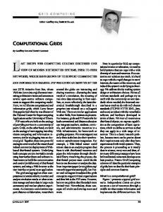
2. Model The Grid contains m machines. We say that machine Mi has size mi if it comprises mi processors. All processors in the Grid are identical. For the purpose of easier descriptions, we assume a machine indexing such that mi−1 ≤ mi holds and introduce m0 = 0. We use GPm to describe the Grid machine model. Jobs are independent and submitted over time. Job Jj is characterized by its processing time pj > 0, its submission time rj ≥ 0, and its fixed degree of parallelism sizej ≤ sm , that is the number of processors that must be exclusively allocated to the job during its processing. We consider nonclairvoyant scheduling that is, the processing time of a job only becomes known after a job has completed its execution. Further, we allow neither multisite scheduling nor preemption, that is, job Jj must be executed on sizej processors on one machine without interruption. We introduce the notation i = a(j) to indicate that job Jj will be executed on machine Mi . The completion time of job Jj in schedule S is denoted by Cj (S). However, we may simply use Cj if the schedule is non ambiguous. A schedule is feasible if rj + pj ≤ Cj holds for all jobs Jj and if at all times t and for each machine Mi , at most mi processors are used on this machine Mi , that is, we have X mi ≥ sizej Jj |Cj −pj ≤t 1 be an integer. In our Grid, we assume one machine Mm with mm = 2k processors, and there are 2 · 4κ−1 identical machines with 2k−κ processors for each κ with 1 ≤ κ ≤ k. This yields a total of 22k k processors and m = 1 + 2 4 3−1 machines in the Grid. Further, we have 22(k−κ) jobs with sizej = 2κ for all k+1 0 ≤ κ ≤ k resulting in a total of 4 3 −1 jobs. All those jobs have pj = 1. Assume that the jobs are sorted by parallelism in ascending order. Then list scheduling will start all jobs with sizej = 1 concurrently at time 0 on all machines. At time 1, all jobs with sizej = 2 begin their processing on all machines with mi ≥ 2 while all machines with mi = 1 must remain idle. The process repeats until finally, the last job with sizej = 2k starts at time k on machine Mm yielding Cmax = k + 1, see Fig. 1. However, if the list is sorted by parallelism in descending order then each job Jj is allocated to a machine Mi such that size and parallelism match (sizej = ma(j) ). This ∗ produces the optimal makespan Cmax = 2.

(a) List schedule

(b) Optimal schedule Figure 1. Schedules of Example 4.1: (a) Worst Case List Schedule (b) Optimal Schedule

Obviously, this result is due to a load imbalance as machines with many processors execute jobs with little parallelism causing parallel jobs waiting for execution. This observation suggests to sort the list by job parallelism in descending order such that highly parallel jobs are scheduled first whenever there is a choice. Unfortunately, this approach does not guarantee a constant competitive factor either. As a comprehensive example is rather complicated we explain the two main parts of the example separately. Example 4.2 demonstrates that list scheduling may still prevent several parallel jobs being executed concurrently on a single machine even if the list is sorted by job parallelism in descending order. Example 4.2 Consider machine Mi in the Grid such that µ is the number of processors of the largest machine with less processors than mi . For each k with µ + 1 ≤ k ≤ mi − 1, we have one job Jj with a very small processing time (pj → 0) and sizej = k. The small processing time assures that the execution of these parallel jobs does not require much time although they must be executed one after the other. Further, there is a large number of sequential jobs (sizej = 1) with various processing times. As we address nonclairvoyant scheduling the sequential jobs cannot be distinguished at the time of scheduling. We assume that the processing times of the sequential jobs are large enough such that each sequential job completes after the last of the above mentioned parallel jobs has completed. List scheduling with sorting by parallelism in descending order will start the job with sizej = mi −1 at time 0. At the same time, a sequential job is started as no parallel job fits onto this machine anymore. After completion of the parallel job, the algorithm concurrently starts the job with sizej = mi −2 and another sequential job. This process is continued and produces a schedule in which a job with sizej = µ + 1

si =9

Figure 2. Schedule of Example 4.2

is running concurrently with mi − µ − 1 sequential jobs, see Fig. 2. This situation will not change later unless at least two sequential jobs complete at the same time. Due to the small processing time of the parallel jobs, the execution of this schedule takes only very little time. If there are several machines with the same number of processors, we simply multiply the jobs accordingly. Due to Example 4.2, we can now consider an example where list scheduling is based on sorting by parallelism in descending order, and on each machine Mi with mi > 1, one parallel job is started concurrently with several sequential jobs almost at time 0. Example 4.3 Let k > 2 be any integer. Our Grid contains k different types of machines such that there are bκ ma(κ+2)(κ−1) 2 for each 1 ≤ κ ≤ k. We chines of size mκ = 2 say that these machines have type κ. Further, there are aκ jobs of type κ for each 1 ≤ κ ≤ k, that is, those jobs have κ(κ−1) parallelism sizeκ = 2 2 . Note that

mκ sizeκ

=

2

(κ+2)(κ−1) 2

2

κ(κ−1) 2

= 2κ−1

jobs of type κ can be executed concurrently on a machine of type κ. All jobs have a processing time of about 1. However, the processing times are selected such that no two jobs complete at exactly the same time on the same machine in list schedule S. In the optimal schedule, only jobs of type κ are executed on machines of type κ. This promκ ∗ = bκ · 2κ holds for all duces Cmax ≈ 2 if aκ ≤ 2bκ · size κ 1 ≤ κ ≤ k and if there is at least one κ with aκ > bκ · 2κ−1 . In list schedule S, only one job of type κ is started on each machine of type κ at approximately time t with t < κ − 1 being a non negative integer. At approximately time κ, all remaining jobs of type κ are started on all machines of type κ or higher such that at most sizeκ processors become idle on any such machine at the same time for κ 6= k, see Fig. 3. This schedule has the makespan Cmax (S) ≈ k. Finally, we need to determine appropriate values for aκ and bκ . To this end, we use a backward recursion: bk = 1 and ak = 2k−1 + k − 1. For 1 ≤ κ < k, we select Pk bκ

=

h=κ+1 bh

d Pk

aκ

=

κ sizeκ mκ aκ bκ

· (mh − sizeh ) e mκ − sizeκ (κ − 1)

h=κ+1 bh

· (mh − sizeh ) + sizeκ mκ +bκ (κ − 1 + ). sizeκ

Note that this selection is always possible as we have mκ 2i − i ≥ 1 for all non negative integer i. Further, bκ size < κ mκ aκ ≤ 2bκ sizeκ holds for all 1 ≤ κ ≤ k. Table 1 gives the numbers for k = 3 and k = 4. As this example already requires very large numbers of machines and jobs even for a small k, it is mainly of theoretical interest. Also note that this list scheduling algorithm is not a distributed one. Example 4.3 indicates that it may be difficult to determine a fixed order of the job list to guarantee a constant competitive factor for the Grid scheduling problem. Therefore, Grid scheduling is more difficult than multiprocessor scheduling.

5. Grid Scheduling Algorithm As conventional list scheduling is not suitable for Grids, we present an approach that uses several lists. Each of these lists does not require any specific order. We start by

κ sizeκ mκ aκ bκ

1 1 1 4480 2240

1 1 1 112 56

2 2 4 56 14

2 2 4 2240 560

3 8 32 6 1

3 8 32 224 28

4 64 512 11 1

Table 1. Parameters of Example 4.3 with k = 3 and k = 4

adopting the commonly known lower bound for the optimal makespan in the concurrent-submission case to the Grid scheduling problem: P j|sizej >mi−1 pj · sizej ∗ Pm Cmax ≥ max{max pj , max } j 1≤i≤m ν=i mν (1) Compared to the bound of the Pm ||Cmax problem, this bound also considers the unavailability of small size machines for the processing of highly parallel jobs due to the lack of multisite job execution. The Grid scheduling algorithm is based on different initial allocations of the jobs to the various machines. Those allocations are represented with the help of job categories for each machine. Definition 5.1 For every machine Mi , there are three different categories of jobs: 1. Ai = {Jj | max{ m2i , mi−1 } < sizej ≤ mi } 2. Bi = {Jj |mi−1 < sizej ≤

mi 2 }

3. Hi = {Jj | m2i < sizej ≤ mi−1 } Set Ai contains all jobs that cannot execute on the previous (next smaller) machine and require more than 50% of the processors of machine Mi . Set Bi contains all jobs that cannot execute on the previous machine but require at most 50% of the processors of machine Mi . Set Hi contains all jobs that require more 50% of the processors of machine Mi but can also be executed on the previous machine. Note that for each job Jj , there is exactly one index i with mi−1 < sizej ≤ mi as the mi are ordered. If mi−1 ≥ mi 2 then we have Jj ∈ Ai otherwise job Jj is either in Ai or in Bi . Therefore, each job Jj belongs to exactly one category A or B. Obviously, either Bi = ∅ or Hi = ∅ hold for each machine Mi . A job in category Bi cannot

1 1

56

S1=1

2

S2=4

1

14

3

S3=32 (a) List schedule

2 56

S1=1

2

1 1

S2=4

14

2

S3=32 (b) Optimal schedule

Figure 3. Schedules of Example 4.3 for k = 3: (a) Worst Case List Schedule (b) Optimal Schedule

Algorithm Grid Concurrent-Submission

Procedure Update

for i ← 1 to m do Li ← Ai S i ← Hi endfor Update repeat for i ← 1 to m do while enough processors are idle on machine i do schedule a job from Li on machine i remove the scheduled job from all lists Lk if any list Lk = ∅ Update endif endwhile endfor until all jobs are scheduled

for i ← 1 to m do if Li = ∅ if i 6= 1 and Si 6= ∅ Li ← Li−1 ∩ Si Si ← Si \ Li elseif Bi 6= ∅ Li ← Bi endif if i 6= 1 and Li−1 6= ∅ and Si = ∅ Li ← Li−1 endif endif

Figure 4. Grid Scheduling Algorithm for the Concurrent-Submission Case (rj = 0)

belong to any other category while a job in category Hi must also belong to either category Ai−1 or category Hi−1 . Therefore, Hi ∩ Hi−1 6= ∅ requires Ai−1 ⊆ Hi . Next, we present the Grid scheduling algorithm for the concurrent-submission case in Fig. 4. This algorithm uses a main list Li and a support list Si for each machine Mi . List Li contains all jobs that are ready for scheduling on machine Mi while list Si simply keeps track of the jobs in Hi that have not yet been transferred to Li . Note that a job may be on the lists of several machines at the same time. Procedure Update in Fig. 5 is a key component of the algorithm. It maintains the lists of the various machines. If there is no job ready for scheduling on machine Mi (Li = ∅) then jobs from Hi are enabled for scheduling on machine Mi if they are already available for scheduling on machine Mi−1 . If this type of job does not exist (Hi = ∅) and no jobs are ready for scheduling on machine Mi then all jobs in Bi are enabled for scheduling on machine Mi . Note that it is important to process these sets in ascending order of machine indexes when using the sequential program notation. We assume that the processing time of this procedure does not introduce any additional idle time into the schedule. Also remember that it is not the intention of this paper to present an efficient implementation of the procedure but to demonstrate the algorithmic concept. Consider a job j that is in Hi and Ai−1 . The algorithm places this job into Li−1 during startup. Procedure Update will enter it into Li once all jobs from Ai are scheduled unless j has already started. A job j ∈ Hi+1 ∩ Ai−1 will become element of Li+1 once all jobs from Ai+1 and

Figure 5. Update of Lists for the ConcurrentSubmission Case

Ai ∩Hi+1 are scheduled and so on. Procedure Update guarantees that a list Li is not empty if there is a job in any list Li0 with i0 < i. Algorithm Grid Concurrent-Submission in Fig. 4 first initializes the lists Li and Si for all machines. As list Li may be empty for some machines, Procedure Update is also called once immediately afterwards. Later, Procedure Update is called again if the last job of a list Li has been started on any machine. Next, we show that Algorithm Grid ConcurrentSubmission prevents intermediate schedule intervals with the majority of processors of a machine being idle. Lemma 5.2 Algorithm Grid Concurrent-Submission guarantees that on every machine in the Grid more than 50% of its processors are always busy executing jobs before the starting time of the last job on this machine. Proof. Assume that we have • at least m2i idle processors on some machine Mi at some time t and • a job Jj with Cj − pj > t and a(j) = i. Remember that jobs from Ai and Hi are scheduled on machine Mi first. Therefore, more than m2i processors are always busy on machine Mi until all jobs from Ai and Hi are completed. Further, no job requiring at most m2i processors can still be on list Li at time t as enough processors are idle to start this job immediately. Therefore, list Li must be empty at time t. As job Jj is still unscheduled at time t it must belong to Ai0 \Hi or to Bi0 for some machine Mi0 with i0 < i resulting in Li0 6= ∅ at time t . However, procedure Update guarantees that list Li is not empty if there is a job in any list Li00 with i00 < i. This is a contradiction. u t

Unfortunately, Examples 4.1 and 4.3 demonstrate that Lemma 5.2 is not sufficient to prove a constant competitive factor. In addition, we need a balanced “utilization” of the machines in the Grid. In Lemma 5.3, we demonstrate that in case of an unbalanced utilization, no resources of highly parallel machines are wasted to execute jobs with little parallelism. Lemma 5.3 Let Jj 0 be any job with Cj 0 (S) = Cmax in a schedule S produced by Algorithm Grid ConcurrentSubmission. If there is a machine Mi with i < a(j 0 ) and at least m2i processors being idle at time t < Cj 0 −pj 0 then Algorithm Grid Concurrent-Submission will produce a schedule S 0 with the same makespan (Cmax (S 0 ) = Cmax (S)) if all jobs in sets Ai0 and Bi0 with i0 ≤ i are removed. Proof. The claim is clearly correct if no machine Mk with k > i executes any job in sets Ai0 or Bi0 with i0 ≤ i. Let us assume that there is a job Jj in set Ai0 or set Bi0 with i0 ≤ i and that this job is executed on machine Mk with k > i. Due to Procedure Update, job Jj can only enter Lκ for some i < κ ≤ k if all jobs from Aκ and Bκ are already scheduled. Therefore, removing all jobs in categories Ai0 and Bi0 with i0 ≤ i will not influence the completion time of any job in sets Aκ and Bκ with i < κ ≤ k. Finally, we have Jj 0 ∈ Aν or Jj 0 ∈ Bν for some machine Mν with ν > i as job Jj 0 did not start on machine Mi at or before time t. Therefore, the removal of all jobs in sets Ai0 and Bi0 with i0 ≤ i cannot reduce Cmax (S). u t Now, we are ready to prove the competitive factor of Algorithm Grid Concurrent-Submission. Theorem 5.4 Algorithm Grid Concurrent-Submission max guarantees C < 3 for all input data and all Grid ∗ Cmax configurations in the concurrent-submission case. Proof. Let Jj 0 be any job with Cj 0 (S) = Cmax in a schedule S produced by Algorithm Grid Concurrent-Submission. If there is a machine Mi with i < a(j 0 ) and at least m2i processors being idle before Cj 0 − pj 0 then we remove all jobs in sets Ai0 and Bi0 with i0 ≤ i. This does not reduce the Cmax ratio C as Cmax remains unchanged due to Lemma 5.3 ∗ max ∗ and Cmax cannot increase. If necessary we can execute this process repeatedly. Due to Lemma 5.3, we can assume that there is a machine Mk such that for each machine Mκ with k ≤ κ ≤ a(j 0 ), more than 50% of the processors are always busy before time Cj 0 − pj 0 and that all machines Mi0 with i0 < k can be ignored for the purpose of the analysis as they cannot execute any job from Aκ and Bκ with κ > k. Now assume that there is some time t < Cj 0 − pj 0 such that at most 50% of the processors of some machine Mi0 with i0 > a(j 0 ) are executing jobs at t in S. Then we have

Li0 = ∅ and La(j) 6= ∅ at t. Again this is not possible due to the execution of Procedure Update. This leads to

Cmax (S)

= pj 0 + Cj 0 − pj 0 P < pj 0 + 2 ·

Jj ∈Aν ∪Bν |ν≥k

P

pj · sizej

ν≥k mν

∗ ∗ ∗ ≤ Cmax + 2Cmax = 3Cmax .

u t However, the ratio of Theorem 5.4 is not tight. Intuitively, tightness would require a Grid schedule with only 50% of the processors being used while the optimal schedule executes the same jobs without idle processors. In addition, at the end of the Grid schedule, there must be another long running job that cannot start earlier. We are not able to find such a problem instance but we can present an example showing that this algorithm produces competitive ratios that come arbitrarily close to 2.5 for some input data and Grid configurations. Example 5.5 Consider a simple Grid mit m = 2, m1 = 1, and m2 = 21. There are 7 jobs in A1 : 6 identical jobs with sizej = 1 and pj = 1, and the last job in this list with sizej = 1 and pj = 4. There are 2 jobs in A2 : the first job with sizej = 11 and pj = 3, and the last job with sizej = 11 and pj = ² → 0. Finally, B2 contains first one job with sizej = 8 and pj = 3, then three identical jobs with sizej = 7 and pj = 1, and at the end, one job with sizej = 8 and pj = ² → 0. Both jobs with pj = ² are only necessary to prevent that A2 and B2 become empty prematurely. In schedule S, all jobs in A1 are assigned to machine M1 . The longest running job starts last at time 6 and determines the makespan Cmax (S) = 10. This is only possible if L2 does not become empty before time 6. The long running job in A2 starts at time 0 and the other one follows immediately. Therefore, B2 becomes L2 at time 3 and the first job of B2 starts at time 3 and completes at time 6. The next three jobs of B2 execute concurrently to the first job and start at times 3, 4, and 5, respectively while the last one starts at time 6, see Fig. 6. Hence, L2 becomes empty at time 6. ∗ It is easy to assemble an optimal schedule with Cmax = 4 + ², see Fig. 6. This produces a ratio of Cmax (S) ∗ ²→0 Cmax lim

=

10 = 2.5. ²→0 4 + ² lim

A more complicated example yields a lower bound for the competitive factor of Algorithm Grid ConcurrentSubmission that comes arbitrarily close to 21 8 = 2.625.

10

6 3

2

21

10 (a) Grid schedule

3

2

10

21

(b) Optimal schedule

Figure 6. Schedules of Example 5.5: (a) Schedule of Algorithm Grid Concurrent-Submission (b) Optimal Schedule

6. General Problem with Submission over Time Finally, we address the general submission-over-time problem. Algorithm Grid Concurrent-Submission can be modified to solve this problem by using the results of Shmoys, Wein, and Williamson [11]. This will increase the (S) competitive factor by a factor of 2 and result in Cmax < ∗ Cmax 6. However, in practice, this kind of algorithm is hardly acceptable as it requires newly submitted jobs to wait for a significant time span even if the job is not highly parallel and enough processors are available. Therefore, we want to examine a simple modification of Algorithm Grid Concurrent-Submission that generates a better competitive factor and may be more relevant in practice. First, we change sets A, B, and H from being static to being dynamic: Once a job is scheduled it is removed from all sets and lists. On the other hand, any newly submitted job is introduced into the appropriate sets. Note that the difference between Hi and Si becomes smaller but it still exists as a job is removed from Hi after scheduling and from Si after being introduced into Li , respectively. Second, we modify Algorithm Grid ConcurrentSubmission by deleting all lists Li and Si whenever a new job is submitted and restarting the procedure Update for initialization purposes. We call the resulting method Algorithm Grid Over-Time-Submission. Certainly, an suitable implementation can avoid some of those list modifications

and execute other modifications in an efficient manner. But it is not the intention of this paper to address implementation efficiencies. The performance analysis of Algorithm Grid Over-TimeSubmission is heavily based on the analysis of Algorithm Grid Concurrent-Submission in Section 5. Theorem 6.1 Algorithm Grid Over-Time-Submission max guarantees C < 5 for all input data in the over-time∗ Cmax submission case. Proof. Let assume that r is the submission time of the last job in schedule S. After time r, the mechanisms of Algorithm Grid Concurrent-Submission apply. However, while Algorithm Grid Concurrent-Submission was previously starting with all processors being idle now processors may be busy executing some jobs that have been submitted earlier. Jobs from sets A or H may have to wait until enough processors are available. During this time, m2i processors or more may be idle on machine Mi . But as all lists Li have been emptied this time span is limited to the maximum processing time of any job. Therefore, the conditions of Lemmas 5.2 and 5.3 apply after time r + maxj pj at the latest. As the bounds of Equation (1) and inequality ∗ r < Cmax hold in the over-time-submission case and we have Cmax (S)

∗ ∗ < r + max pj + 3Cmax < 5Cmax . j

u t

As with Algorithm Grid Concurrent-Submission the bound of Theorem 6.1 is not tight. But it is possible to show that the lower bound for the competitive factor of Algorithm Grid Over-Time-Submission comes close to 4.5.

7. Conclusion In this paper, we present a Grid model that covers the main properties of Grid computing systems in our view. Based on this model, we analyze a fundamental Grid scheduling problem that has been derived from one of earliest and most basic multiprocessor scheduling problems. To our knowledge, this is the first comprehensive theoretical analysis of Grid scheduling. We show that Grid scheduling is more complex than the corresponding multiprocessor scheduling problem and that the well known list scheduling algorithm cannot guarantee a constant competitive ratio for the makespan, although it performs very well in the multiprocessor case. This result even holds if the list is sorted by job parallelism in descending order. The given examples seem to indicate that no static list ordering based on job parallelism can guarantee a good Grid schedule independent of the Grid configuration. Further, we present a new algorithm that is based on several lists and guarantees a competitive ratio of 3 in a scenario with all jobs being submitted concurrently. As we consider nonclairvoyant jobs this problem also has some online properties. Then we extend this algorithm to the general submission-over-time scenario producing a competitive factor of 5. To our knowledge, this is first time a constant competitive factor has been proved for this type of problem. Although we do not address implementation details of our algorithms in this paper we like to point out that significant parts of our algorithm can be implemented in a distributed fashion: Each machine has its own job lists and only schedules jobs from these lists. Originally, each job is allocated to exactly one list Ai or Bi . Assuming a global Grid information system this can be achieved using a simple master-slave approach. If there are no jobs available in the lists of a machine, this machine starts to use the list of a neighboring machine resulting in local communication only, that is, a machine may “steal” a job from a neighbor. But dynamic information regarding the availability of jobs must still be shared among several machines. Although implementing the algorithm by using job stealing from a neighboring machine may influence the quality of the schedule in practice, the algorithm seems suitable for implementation in real systems. But in these real systems, other properties of computing Grids must be considered as well. Nevertheless, the proposed algorithm may serve as a starting point for heuristic scheduling algorithms that are implemented in real computing Grids.

References [1] S. Albers. Better bounds for online scheduling. SIAM Journal on Computing, 29(2):459–473, 1999. [2] I. Foster and C. Kesselman, editors. The GRID: Blueprint for a New Computing Infrastructure. Morgan Kaufmann, 1998. [3] N. Fujimoto and K. Hagihara. Near-optimal dynamic task scheduling of independent coarse-grained tasks onto a computational grid. In Procedings of the 32nd Annual International Conference on Parallel Processing (ICPP-03), pages 391–398. IEEE Press, October 2003. [4] M. Garey and R. Graham. Bounds for multiprocessor scheduling with resource constraints. SIAM Journal on Computing, 4(2):187–200, June 1975. [5] R. Graham, E. Lawler, J. Lenstra, and A. R. Kan. Optimization and approximation in deterministic sequencing and scheduling: A survey. Annals of Discrete Mathematics, 15:287–326, 1979. [6] C. B. Lee, Y. Schwartzman, J. Hardy, and A. Snavely. Are user runtime estimates inherently inaccurate? In Proceedings of the 10th Workshop on Job Scheduling Strategies for Parallel Processing, pages 153–161, June 2004. [7] E. Naroska and U. Schwiegelshohn. On an online scheduling problem for parallel jobs. Information Processing Letters, 81(6):297–304, March 2002. [8] M. Pinedo. Scheduling: Theory, Algorithms, and Systems. Prentice-Hall, New Jersey, second edition, 2002. [9] T. Robertazzi and D. Yu. Multi-Source Grid Scheduling for Divisible Loads. In Proceedings of the 40th Annual Conference on Information Sciences and Systems, pages 188–191, March 2006. [10] U. Schwiegelshohn and R. Yahyapour. Attributes for communication between grid scheduling instances. In J. Nabrzyski, J. Schopf, and J. Weglarz, editors, Grid Resource Management – State of the Art and Future Trends, pages 41–52. Kluwer Academic, 2003. [11] D. Shmoys, J. Wein, and D. Williamson. Scheduling parallel machines on-line. SIAM Journal on Computing, 24(6):1313–1331, December 1995. [12] A. Tchernykh, J. Ramrez, A. Avetisyan, N. Kuzjurin, D. Grushin, and S. Zhuk. Two level job-scheduling strategies for a computational grid. In R. Wyrzykowski, J. Dongarra, N. Meyer, and J. Wasniewski, editors, Proceedings of the 2nd Grid Resource Management Workshop (GRMW’2005) in conjunction with the 6th International Conference on Parallel Processing and Applied Mathematics - PPAM 2005, pages 774–781. Springer–Verlag, Lecture Notes in Computer Science 3911, September 2005.