for pricing an option, using online trading algorithms. Our bounds depend on very ... âGraduate School of Business, Stanford University. â Graduate School of .... pared to the best asset in hindsight, namely max {100, ST }.) By scaling our online ...
Online Trading Algorithms and Robust Option Pricing Peter DeMarzo∗
Ilan Kremer†
ABSTRACT In this work we show how to use efficient online trading algorithms to price the current value of financial instruments, such as an option. We derive both upper and lower bounds for pricing an option, using online trading algorithms. Our bounds depend on very minimal assumptions and are mainly derived assuming that there are no arbitrage opportunities.
General Terms Algorithms, Theory, Economics
Categories and Subject Descriptors I.2.6 [Learning]; F.2.2 [Nonnumerical Algorithms]; J.4 [Economics]
Keywords Finance, Online Algorithms, Regret Minimization
1.
INTRODUCTION
Options have been used from the time of Ancient Romans, Grecians, and Phoenicians for risk management. A call option is a contract between two parties (buyer and seller, or writer) that provides the buyer with insurance against appreciation in the price of a risky asset. It is used to hedge risk associated with financial assets (such as equities and ∗
Graduate School of Business, Stanford University Graduate School of Business, Stanford University. Part of the work was done while the author was a fellow in the Institute of Advance studies, Hebrew University. ‡ School of computer Science, Tel-Aviv University. Part of the work was done while the author was a fellow in the Institute of Advance studies, Hebrew University. This work was supported in part by the IST Programme of the European Community, under the PASCAL Network of Excellence, IST-2002-506778, by a grant no. 1079/04 from the Israel Science Foundation and an IBM faculty award. This publication only reflects the authors’ views. †
Permission to make digital or hard copies of all or part of this work for personal or classroom use is granted without fee provided that copies are not made or distributed for profit or commercial advantage and that copies bear this notice and the full citation on the first page. To copy otherwise, to republish, to post on servers or to redistribute to lists, requires prior specific permission and/or a fee. STOC’06, May21–23, 2006, Seattle, Washington, USA. Copyright 2006 ACM 1-59593-134-1/06/0005 ...$5.00.
Yishay Mansour‡
currencies) as well as non-financial assets (commodities such as oil). A (European) call option on a risky asset gives you the right but not the obligation to buy a risky asset on a prespecified date, T , at a pre-specified price, K, referred to as the strike price. For example, a T = 1-year call option on IBM with a strike price K = $100 gives you the right but not the obligation to buy an IBM share from the writer of the option for a price of $100. If we denote the value of the risky asset at time t by St then at time T the payoff of the call option is given by: max{ST − K, 0}. A fundamental question in finance is to determine the value of such an option today. This research question (which has many practical implications) has been a source of one of the main achievements in economics. Black and Scholes [3] studied this question in a path breaking paper that was later recognized by the 1997 Noble Prize. They show how one can replicate the payoff of an option using a dynamic trading strategy; based on this they provide an exact current valuation of the option. Their approach uses a no arbitrage condition and is based on the assumption that the logarithm of the stock price follows a certain continuous time version of a random walk1 . They also assume that the stock and a risk free bond can be traded continuously. Our bounds use a no arbitrage assumption, which implies the following. If there are two securities A1 and A2 , such that the payoff of A1 always dominates the payoff of A2 (on any future outcome), then the current value of A1 is at least that of A2 . (Intuitively, one can always buy A1 rather than A2 and guarantee at least the same payoff.) The Black and Scholes assumption on the stock price process is an important limitation of the Black and Scholes model. In practice share prices exhibit behavior that is not consistent with the simple random walk assumption made by the Black and Scholes model. Most importantly, trading is discrete and the price paths are discontinuous and include price jumps. Since Black and Scholes, there has been much research both in extending the results to alternative stock price processes, and in examining the empirical performance of the resulting valuation models. (We review briefly some of the related finance research in the Appendix.) The main goal of our work is to provide robust upper and lower bounds for European call options. The bounds we provide are robust in the sense that we do not restrict the form of the 1 More specifically they assume geometric Brownian motion with a drift; for more details see, for example, [12].
stock price process, we do not require continuous trading, and we allow for price jumps. At this point it would be worthwhile to define our notation. We assume that the risky asset at time t is valued at St = St−1 (1 + rt ), and that the returns rt are bounded by some constant M , i.e., |rt | ≤ M . We call the sequence of rt ’s the price path. Let C(K, T ) be the current price of an option with a strike price K that matures at time T , i.e., at time T the option payoff is max{ST −K, 0}. We also assume a risk free asset is available and it pays a constant interest rate rf . For convenience, we normalize the interest rate to be zero (and later show how to relax this assumption). We make two assumptions regarding the price path. Our main assumption P 2 bounds the quadratic variation of the risky asset, i.e., t rt . Specifically for our upper bound on the option price we use an assumption of the form: 2 T X
rt2 < Q.
t=1
We make an additional assumption regarding to the maximal single-period return of the stock by restricting |rt | ≤ M . However this bound is weak and has a very mild effect on our price bounds for the option. (Black and Scholes effectively restrict M = 0 as they require continuous price paths.) Unlike the Black and Scholes model, in our case we make no further assumptions on the underlying process, and allow for both price jumps and discreteness in trading. The advantages of our bounds is that they apply in a very adversarial setting, where the only restriction on the adversary is regarding the maximum quadratic variation and maximal single-period return. Another advantage is that the bounds are dependant on the quadratic variation in discrete time, which imply that if we make the trading less frequent our bounds do not deteriorate significantly. When examining our bound it is important to note that without bounding the quadratic variation there is little we can say about the value of the call option. As Merton [27] shows one can only say that the value of a call option cannot be higher than the current share price S0 and cannot be negative or lower than the difference between the current share price and the strike price. Hence, the bound for the value of a call option is given by: C(K, T ) ∈ [max {0, S0 − K} , S0 ] . The above bound is based on an arbitrage condition; if the price of the call option is outside this range then one can construct an arbitrage strategy that is guaranteed to make money. These bounds are tight as there does not exist an arbitrage for prices in this set if we do not put any restriction on the price path of the risky asset. In this work we demonstrate that it is possible to significantly improve on these bounds by assuming an upper bound on the quadratic variation and the maximal single-period return. Our approach is based on online algorithms and in particular the best expert problem [26, 5, 19, 1, 6] and regret minimization ideas [17, 18, 20, 25]. To illustrate our approach consider the following example. Suppose the current 2 The quadratic variation is closely related to the volatility parameter in the Black and Scholes model. In the Black-Scholes setting the quadratic variation converges to the stock’s volatility when we observe the stock price at finer and finer time increments; hence, in practice quadratic variation is often used to estimate volatility.
IBM share price is $100 and the risk free interest rate is zero. Assume that we have an online trading algorithm such that if we start with $100 then at time T our payoff will exceed max {80, 0.8ST }, where ST denotes IBM share price at time T . (This can be viewed as a loss of not more than 20% compared to the best asset in hindsight, namely max {100, ST }.) By scaling our online trading algorithm we can conclude that starting with $125 our algorithm would have a payoff that exceeds max {100, ST }. If we borrow $100 to initiate our online algorithm, then after paying off our (zero interest) loan, the final payoff of our online algorithm would exceeds max{0, ST − 100}, which is identical to the payoff of a call option on IBM with a strike price of $100. Thus, to avoid arbitrage, the value of the call option cannot exceed the upfront cost of $25 of the online trading algorithm. In the above example the quality of our bound is determined by the loss of our online trading algorithm relative to best static decision (which is either to buy the stock or not to buy it). A loss of 20% translated into a bound of $25 and a better guarantee would translate into a lower loss and hence better (i.e., lower) upper bound. In our analysis we use online algorithms to minimize the loss given a bound on the quadratic variation of the risky asset. As a first step in constructing our upper bound, we derive an online trading algorithm generic that has a relatively small loss. The generic online trading algorithm, assuming that the quadratic variation is bounded by Q, ends with value GT , and has a guarantee of ln(GT ) ≥ max{ln(ST ) −
1 1 1 1 ln − (η − 1)Q , − ln }, η w η 1−w
where we normalize S0 = 1, and both w ∈ (0, 1) and η ≥ 1 are parameters of the algorithm. Given the generic online trading algorithm we derive the upper bound for the price of the call option. By varying the parameters of the algorithm, we are able to produce upper bounds for the entire range of possible strike prices. We also show how to incorporate non-zero interest rates in our model. Furthermore, we show that we can integrate other assumptions to get improved bounds, for example by assuming an upper or lower bound on the final risky asset price ST . Finally, we discuss and compare our bounds to that of Black and Scholes.3 We study the optimal bound that one can derive for a given maximal single-period return M and a quadratic variation bounded by Q. We model the optimal bound as a finite horizon zero-sum game. Using basic properties from game theory, as well as the no arbitrage condition, we are able to significantly simplify it. Using a dynamic programming approach for the simplified form, we derive a polynomial time approximation for this optimal bound (given M , Q and T ). The optimal bound is interesting both from a finance perspective and a computational perspective. From the finance perspective it allows us to compare the resulting bound with existing evaluations, most importantly the Black and Scholes one. From a computational perspective it gives us a meaningful benchmark for our online algorithm. 3 One of the main advantage of our bounds is that since they depend on the quadratic variation, they allow for a very natural comparison to the standard literature in finance which uses volatility.
We also derive a universal lower bound on the price of an option. Specifically, we show that if the price path is guaranteed to have a quadratic variation of at least Qmin , then the value of the option must exceed this lower bound.4 In order to derive the lower bound we need to demonstrate an online trading strategy that would have a “guaranteed loss”, regardless of the future outcomes. Based on such an online trading strategy and the no arbitrage assumption, we derive our lower bound. Note that our lower bound is not limited to a specific instance of prices but rather provides a no-arbitrage lower bound. As mentioned earlier, our research builds on existing results in online learning and in particular regret minimization. The regret minimization problem has been extensively studied in the computational learning theory community and tight bounds have been derived on its behavior [26, 5, 19, 1]. In a nutshell, one can reach almost the gain of the best action, assuming that we are allowed to output a linear combination of the actions (or alternatively allowed to use randomization). More precisely, if the gain of the best action is G, then there √ exists an online algorithm whose gain is at least G − O( G log N + log N ). Common to much of the previous computer science work on online trading algorithms is the goal of beating the market. To do so requires designing an online algorithm that can have a guarantee of performing very well in the market, even under adversarial conditions. Much of the Finance literature assumes that assets are priced fairly, and at the very least assumes that there are no arbitrage opportunities, which implies that no online algorithm can “beat the market”. A significant conceptual contribution of our work, to the computer science view point, is that efficient online algorithms can play an important role even if we assume no arbitrage in the market prices. Our goal is much more modest, we try to price fairly a given financial instrument, and to this end we do need to design efficient online algorithms. Another observation is regarding the static adversary in the online model. Essentially, an option is an “insurance” contract to get the performance of a static adversary, which in hindsight selects between the risky and risk free asset. While in much of the competitive online literature a static adversary is viewed as an extremely limited adversary, in the finance setting it has both a very natural interpretation and very significant applications. We briefly outline the main research direction in online algorithms regarding financial problems. The universal portfolio, proposed by [9] and latter studied in [4, 24, 33, 21, 10, 11, 35], has been one of the well studied finance problem in the information theory and computer science literature. In this setting the aim is to devise an online trading algorithm that is competitive against any constant rebalancing portfolio. Another finance-motivated problem that has received considerable attention is the one-way trading problem, first studied in [14], and latter in [7, 13, 22]. In this problem one needs, for example, to change a fixed amount of Yen to Dollars. The aim is to compare well with any trading strategy, even one that knows the future prices and trades at the best price. The results derive competitive online trading algorithms, and are highly related to search problems. Ex4 Note that there are two types of lower bounds. The first exhibits some scenario for the lower bound, while the second type claims that in any scenario the lower bound holds. Our universal lower bound is of the second type.
tensions of the one way trading to two way trading appear in [30, 7, 23], where various limitations are assumed regarding the adversary. (Part of the assumptions are aimed at either bounding the offline benefit or guaranteeing that the online algorithm will not lose any money.)
2. MODEL We consider a discrete-time finite-horizon model in which time is denote by t ∈ {0, 1, . . . , T }. There is a risky asset (e.g., stock) whose value (price) at time t is given by St . We normalize the initial value to one, S0 = 1, and assume that the asset does not pay any dividends. We denote by rt the return between t − 1 and t so that St = St−1 (1 + rt ). We call r1 , . . . , rT the price path . In addition to the risky asset we have a risk free asset (e.g., bond). We denote the price of the risk free asset at time t by Bt , where B0 = 1. We assume that the risk free asset carries a fixed interest rf , i.e., Bt+1 = Bt (1+rf ) = (1+rf )t . Unless otherwise stated, we assume that the risk free rate is zero, i.e., rf = 0, which implies that Bt = 1 for all t. A financial security X has for each price path r1 , ..., rT a payoff of X(r1 , ..., rT ). For example, an option can be described as a financial security. An online trading algorithm starting with $c in cash, has initial value G0 = c. At each period it distributes its current value Gt , between the assets, investing a fraction xt in the risky asset and 1 − xt in the risk free asset. Since we assume zero interest rate, at time t+1 its value is Gt+1 = (xt Gt )(1+ rt )+(1−xt)Gt = Gt (1+xt rt ). Its final value is GT . We refer to a fixed portfolio when the online trading algorithm sets its investments at time t = 0, and does not trade anymore. Formally, it implies that xt+1 = xt (1 + rt )/(1 + xt rt ), since the value of the risky asset changes. Let C(K, T ) be the value, at time t = 0, of an option whose strike price is K that matures at time T . This is the present value (at t = 0) of a time T call option with strike price K. At time T the payoff of the call option is given by max{0, ST − K}. P A price path r1 , . . . , rT is a (Q, M ) price path if Tt=1 rt2 < Q and |rt | < M . In the case of a risky asset and a risk free asset, a (Q, M ) price path means that both the price paths, of the risky asset and the risk free asset, are (Q, M ) price path. (For the risk free asset this means that rf2 T < Q and rf < M , which holds trivially for rf = 0.) We call Q the maximum realized quadratic variation of the risky asset and M the maximal single period return. No Arbitrage Assumption: We assume that there is no arbitrage in the prices. Namely, for any two online trading algorithms (or financial securities) A1 and A2 , that start with cash $c1 and $c2 , if for any price path the future payoff of A1 is always at least that of A2 , then c1 ≥ c2 . (If this were not true and c1 < c2 , assuming that one can sell short assets (and strategies), there would be an arbitrage opportunity: Investing in A1 and shorting A2 would lead to a time 0 gain of c2 − c1 without the possibility of loss in the future.) We will use the no arbitrage assumption on a restricted set of price paths, such as (Q, M ) price paths. This implies that any price path which is not in the set is impossible, and the prices reflect this knowledge.
3. AN ONLINE TRADING STRATEGY In this section we introduce an online trading algorithm
generic. The online algorithm will trade using N different assets, and its goal is to have its value approximate the value of the best asset.5 Later we shall see how a simple application of generic indeed yields the desired upper bound on the price of the option. Notation: We denote by Vi,t the price of asset i at time t. We normalize the initial value of each asset to be one, i.e., Vi,0 = 1. The value at time t satisfies Vi,t = Vi,t−1 (1 + ri,t ), where ri,t ∈ [−M, +M ] is the immediate return of asset i at time t. Online Trading Algorithm: Our online trading algorithm, called generic, maintains weights, {wi,t }. Initially P i wi,0 = 1, where the exact setting is a parameter of the algorithm. The algorithm uses the update rule wi,t+1 = wi,t (1 + ηri,t ), for some parameter η ≥ 0. At time t the algorithm forms a portfolio where the fraction P of investment in asset i is xi,t = wi,t /Wt where Wt = i wi,t . Algorithm’s Value: The value of the assets that the online trading algorithm generic holds at time t is denoted by Gt . Initially, G0 = 1, and Gt = Gt−1 (1 + rG,t ), where the immediate return on our portfolio at time t is rG,t = PN way of describing the evolution of the i=1 xi,t ri,t . Another P value is: Gt = N i=1 (xi,t Gt−1 )(1 + ri,t ) = Gt−1 (1 + rG,t ). The following theorem, whose proof appears in the Appendix, summarizes the performance of our online algorithm, generic. Theorem 1. The generic, with h online trading algorithm i 1 1 (1 − 2(1−M ) , and {w parameters: η ∈ 1, M i,0 }, where )
P
i
wi,0 = 1, guarantees that for any asset i,
1 1 ln(GT ) ≥ ln(Vi,T ) − ln − (η − 1)Qi , η wi,0 √ P 2 , and |ri,t | < M < 1 − 2/2 ≈ 0.3. where Qi = Tt=1 ri,t Our option pricing results will rely on an application of the above theorem to a setting with two assets: a risky asset and a risky free asset. With a slight abuse of notation we let w0 denote the amount invested in the risky asset and assume that we invest 1 − w0 in the risk free asset. Since we assume a zero interest rate we have Qf = 0 for the risk free asset and conclude that: Corollary 2. The online trading algorithm generic, 1 1 (1 − 2(1−M )], and w0 ∈ (0, 1), given parameters: η ∈ [1, M when applied to a risky asset and a risk free asset, guarantees that 1 1 − (η − 1)Q , ln(GT ) ≥ max{ln(ST ) − ln η w0 1 1 − ln }, η 1 − w0 √ P where Q = Tt=1 rt2 , and |rt | < M < 1 − 2/2 ≈ 0.3.
4.
Definition 3. We say that c = C u (K, Q, M, T ) is an upper bound if there exists an online trading algorithm that starts with $c and for all possible (Q, M ) price paths its final payoff, GT , satisfies: GT ≥ max {0, ST − K}. As we shall discuss next, we actually examine an equivalent guarantee as follows: Definition 4. An online trading algorithm has an (α, β) guarantee, if for any (Q, M ) price path its final payoff, GT , satisfies GT ≥ max {α, βST }. To gain some intuition it is better to first examine a very simple trading strategy. Suppose we decide to use a buy and hold strategy in which we invest a fraction β in the risky asset and α = 1 − β in the risk free asset (and do not trade anymore). The future payoff of this fixed portfolio, GT , is GT = α + βST ≥ max {α, βST }
This implies that we implemented an (α, β) guarantee for β = 1 − α. Compare the above to the payoff of a fixed portfolio of β call options each with a strike price of K = α β combined with α invested in the risk free asset. Such a fixed portfolio yields at time T a payoff of exactly HT = α + β max{0, ST − (α/β)} = max {α, βST }. By definition, the current price of this fixed portfolio is α+βC( α , T ). Since β HT ≤ GT , by the no arbitrage assumption, we have, α 1−α α = 1 = S0 α + βC( , T ) ≤ 1 ⇒ C( , T ) ≤ β β β
As mentioned before, S0 is a simple known upper bound on the option price. Our goal is to construct online trading algorithm that starts with $1 and yields a future payoff that exceeds: max {α, βST } , for some α + β > 1. Such an algorithm yields a non trivial bound, as stated in the following claim, Claim 5. Assume all price paths are (Q, M ) price paths. An online trading algorithm with an (α, β) guarantee ensures that for a call option with strike price K = α , we have that β u 1−α 1 C (K, Q, M, T ) ≤ β = β − K. We will use the generic online trading algorithm to generate our upper bounds for the value of the options. The main feature of the generic algorithm is that it tries to match the best of the underlying assets, which intuitively, is what we need to generate our bound. From Corollary 2, for a fixed quadratic variation bound Q, we have, GT ≥ max {α (w0 , η) , β (w0 , η) ST } 1/η
for α(w0 , η) = (1 − w0 )1/η and β(w0 , η) = w0 e−(η−1)Q . Now consider the bound for a given strike price K. We obtain this by solving: β ∗ (K) = max β (w0 , η)
OPTION PRICING: UPPER BOUND
We define our upper bounds using an online trading algorithm. Our bounds are based on an online trading algorithm whose payoff always exceed the option payoff, provided we 5
have a (Q, M ) price path. The fact that this derives an upper bound on the price of an option would follow from the no arbitrage assumption.
The algorithm and analysis is in the spirit of [6], however, note that the model there is additive while the model here is multiplicative, which requires a somewhat different analysis.
η,w0
such
α(w0 ,η) that β(w 0 ,η)
h
can simplify this problem by using w0 : w0 (η, K) =
i
1 1 (1 − 2(1−M ) . One M ) α(w0 ,η) = K to solve for β(w0 ,η)
= K and η ∈ 1,
1 . 1 + K η e−η(η−1)Q
Hence, we need to solve the following maximization, β ∗ (K) = max w0 (η, K)1/η e−(η−1)Q
h
such that η ∈ 1,
1 M
η
�
1−
1 2(1−M )
�i
Theorem 6. Assume that all price paths are (Q, M ) price paths and let β ∗ (K) be the solution to the above optimization, then 1 −K C(K, T ) ≤ C (K, Q, M, T ) ≤ ∗ β (K) u
In order to gain better intuition and understanding regarding our upper bound we derived the following corollary for the case of K = 1 (also referred to as an “at the money” call option). Corollary 7. √ Assume all price paths are (Q, M ) price paths, where M = Q/6, then C(1, T ) ≤ C u (1, Q, M, T ) = √ Θ( Q) The lower bound is derived even in the case of one trading period (i.e., T = 1 and r1 = ±M ), while the upper bound is derived from Theorem 6. In the Appendix we discuss extensions of Theorem 6 to the case of positive interest rates and (known) maximum and minimum prices.
of ∆ is unbounded. To overcome this we would like to bound ∆, and in fact we will “eliminate” it.) Our first step would be to show that the minimax theorem applies to our game. For this we need to rely on a version of the minimax theorem, due to Sion [34], and show that the function f is continuous, quasi-concave in ∆ and r˜, and that the space of distributions r˜ is compact under an appropriate topology (C ∗ ). This establishes the following, f (W, S, K, Q, M, T ) =
sup
inf
r ˜∈Σ(Q,M ) ∆
E[f (W + r˜S∆, S(1 + r˜), K, Q − r˜2 , M, T − 1)] . Next, we observe that f (W, S, K, Q, M, T ) = f (0, S, K, Q, M, T ) − W and f (0, S, K, Q, M, T ) ∈ [0, S], which enables us to show that the extremum values are in the domain, i.e., f (W, S, K, Q, M, T ) =
max
r ˜∈Σ(Q,M )
OPTIMAL BOUNDS
In this section we sketch very briefly our results for deriving the optimal bound of an option given that the price path is a (Q, M ) price path. We start by modeling the optimal bound as a zero-sum game between an investor (option underwriter) and an adversary (the market). The investor selects a strategy (buying and selling of shares) while the adversary selects a (Q, M ) price path. The cost to the investor is the difference between the payoff of the option on the selected price path, and the payoff of its strategy. (The investor would like to minimize its cost, while the adversary would like to maximize it.) While the game can be described as a one-shot game it is more convenient to consider a dynamic (extensive form) representation. In the start of each period the investor decides how many shares to buy, ∆ (which can be also negative, meaning that it sells shares short), then the adversary chooses the period return, r (or more precisely a random variable r˜). Formally, we consider the following recursive definition for the function f (W, S, K, Q, M, T ), which bounds the investor’s cost when the investor starts with $W cash, the stock price is S, the strike price is K, the maximum realized quadratic variation is Q, the maximum single period return is M , and the number of periods is T : For T = 0: f (W, S, K, Q, M, 0) = max{S − K, 0} − W . For T ≥ 1: f (W, S, K, Q, M, T ) = inf ∆ supr˜∈Σ(Q,M ) E[f (W + r˜S∆, S(1 + r˜), K, Q − r˜2 , M, T − 1)], where ∆ ∈ R is the number of shares, r˜ is the random variable that represents the next return, and Σ(Q, M ) is the set √ of random variables whose magnitude is bounded by min( Q, M ). We would like to simplify the definition of f both in order to get a better insight and also in order to derive an efficient algorithm for estimating f . (One problem is that the value
∆
E[f (0, S(1 + r˜), K, Q − r˜2 , M, T − 1) − (W + r˜S∆)] .
We establish a martingale property for the adversary and show that it has to select r˜ such that E[˜ r] = 0. (Otherwise, for any γ > 0 the investor can guarantee an increase of γ in its portfolio value by setting ∆ = γ/E[˜ r ].) Notice that once we have this martingale property, the influence of ∆ diminishes, and we have, f (W, S, K, Q, M, T ) =
max s.t.
r ˜∈Σ(Q,M )
5.
min
E[˜ r]=0
E[f (0, S(1 + r˜), K, Q − r˜2 , M, T − 1) − W ] . Additionally, it is sufficient to consider random variables r˜ whose support includes only √ √ two values, ru ∈ [0, min{M, Q}] and rd ∈ [− min{M, Q}, 0]. This implies that the value of f can be well approximated by discretization of the values of ru and rd to O(T /ǫ) values. Using a dynamic programming, on the discretized values of r˜, we establish, Theorem 8. There exists an O(T 4 /ǫ3 ) time algorithm A such that |A(W, S, K, Q, M, T ) − f (W, S, K, Q, M, T )| ≤ ǫS.
6. A UNIVERSAL LOWER BOUND In this section we derive a lower bound as a function of the minimum realized volatility. It is rather straightforward to derive a lower bound in a specific scenario with a given volatility, an example is the Black and Scholes model provides such a bound since it derives the exact value of the option given a specific stochastic model. In this section we derive much stronger lower bounds. We derive a lower bound for the price of an option assuming that every possible price path has at least some minimum realized volatility Qmin . Definition 9. We say that c = C l (K, Qmin , M, T ) is a lower bound for C(K, T ), if there exists an online trading algorithm that starts with $c and its final payoff, GT , satisfies GT ≤ max {0, ST − K}, for all possible price paths for the P risky asset that satisfy Tt=1 rt2 ≥ Qmin and maximal single period return of M . Again, we construct a strategy that provides an alternative but equivalent guarantee. Claim 10. Assume that there exists an online trading algorithm that starts with $1 and its final payoff is at most , Qmin , M, T ) ≥ 1−α max {α, βST }. Then C( βα , T ) ≥ C l ( α β β
Our bound is interesting when it improves the standard n over o ; that is: , 0 lower bound, max{S0 − K, 0} = max 1 − α β α 1−α > max{1 − , 0}, β β
Theorem 11. Assume that the maximal single period return is M and that any price path has quadratic variation at least Qmin , then
1−(1−ρ/2)e−h(ρ,M )Qmin 1+(ρ/2)−e−h(ρ,M )Qmin 2 2 2
where α =
1−α , α
, h(ρ, M ) = (1−ρ)2 / [2(1+
(1 − ρ) ) (1 + M ) ] ≤ 1/8 and ρ ∈ (0, 1). An implication of the above theorem is the following lower bound for a call option at the money (i.e., K = S0 = 1), Corollary 12. Assume that the maximal single period return is M = 0.25, and that any price path has quadratic variation at least Qmin < 1, then C(1, T ) ≥ C l (1, Qmin , M, T ) = Qmin /10.
7.
BLACK-SCHOLES: COMPARISON
It is interesting to compare the upper bounds on the option price given by the generic algorithm (Theorem 6), the optimal bound (Theorem 8) and the Black-Scholes valuation. By definition, the generic algorithm bound is larger then the optimal bound, which is larger then the Black and Scholes pricing6 , however, the main empirical focus is whether they are qualitatively and quantitatively similar. In Figure 1 we show an empirical comparison of the bounds (where our maximum realized quadratic variation corresponds to the volatility parameter in Black and Scholes). As we can see from the graph, both our bounds are similar in shape to the Black and Scholes pricing, and the optimal bound is very close to the Black and Scholes pricing. We would also like to discuss a more theoretical comparison of the models. Formally the Black and Scholes model is not nested in our model. This is due to the fact that 6
The fact that the Black and Scholes price is not an upper bound, even if one fixes the quadratic variation, can be shown in simple examples, even with T = 2.
Black & Scholes optimal bound generic
0.8 0.7 0.6 0.5 0.4 0.3 0.2 0.1 0
which holds when both α, β ∈ (0, 1). Note that one can guarantee α = 0 and β = 1 by simply only investing in the risky asset. It is our ability to guarantee that both α < 1 and β < 1 simultaneously, that will generate interesting bounds. Hence, the objective is very different from the standard objective in online algorithms. We are interested in guaranteeing a certain “loss” as opposed to guaranteeing a maximal gain. In the Appendix we prove,
C l (K = S0 = 1, Qmin , M, T ) ≥
1 0.9
optiona value
Proof. Consider two online trading algorithms. Algorithm A1 , as stated in the claim, is an online trading algorithm which starts with $1, and whose future payoff is bounded by max{α, βST }. Algorithm A2 buys a fixed portfolio of β call options each with a strike price K = α plus $α β risk free asset. The future payoff of A2 is α +β ·max{0, ST − (α/β)} = max{α, βST }. Since the payoffs of A2 dominates the payoffs of A1 , by the no arbitrage condition we have that , T ) ≥ 1, which proves the claim. α + βC( α β
0
0.5
1 strike price
1.5
2
Figure 1: Graph comparing our upper bounds to Black and Scholes using Q = (0.15)2 , and M = 0.1. Black and Scholes is a continuous time model while we consider a discrete time model. Nevertheless one can overcome this technical difference using the fact the Black and Scholes model is a limit of discrete time models. Black and Scholes model with volatility σ 2 can be expressed as the limit of binomial trees where the quadratic variation is Q = σ 2 and p the single period returns are rt = ± σ 2 /T , as T goes to infinity. Since the bounds we derive do not depend on the number of periods we can conclude that the Black and Scholes price with volatility σ 2 is not higher then our upper bounds when σ 2 is a bound on the quadratic variation. One may wonder about the restriction of the quadratic variation in the context of Black and Scholes. When we look at a geometric Brownian motion at discrete intervals, the increments are normally distributed which may suggest that we allow for unbounded quadratic variation. However, in such a case the discrete Black and Scholes trading strategy fails to replicate the option payoff; moreover, the loss is unbounded. A different way of saying this is that while we can define limits of different sequences of discrete time processes, only particular sequences yield the Black and Scholes equation: i.e. binomial trees. At the continuous time limit almost surely the path is continuous and has a fixed quadratic variation.
8. REFERENCES [1] Peter Auer, Nicol` o Cesa-Bianchi, Yoav Freund, and Robert E. Schapire. The nonstochastic multiarmed bandit problem. SIAM J. on Computing, 32(1), 2002. [2] Antonio E. Bernardo and Olivier Ledoit. Gain, loss and asset pricing. Journal of Political Economy, 108(1):144–172, 2000. [3] Fisher Black and Myron Scholes. The pricing of options and corporate liabilities. Journal of Political Economy, 81(3):637–654, 1973. [4] Avrim Blum and Adam Kalai. Universal portfolios with and without transaction costs. In COLT: Proceedings of the Workshop on Computational Learning Theory, 1997. [5] Nicol` o Cesa-Bianchi, Yoav Freund, David P. Helmbold, David Haussler, Robert E. Schapire, and
[6]
[7]
[8]
[9] [10]
[11]
[12] [13]
[14]
[15]
[16]
[17]
[18] [19]
[20]
[21]
[22]
[23]
Manfred K. Warmuth. How to use expert advice. Journal of the Association for Computing Machinery, 44(3), 1997. Nicol` o Cesa-Bianchi, Yishay Mansour, and Gilles Stoltz. Improved second-order bounds for prediction with expert advice. COLT, 2005. A. Chou, J. Cooperstock, R. El-Yaniv, M. Klugerman, and T. Leighton. The statistical adversary allows optimal money-making trading strategies. In Proceedings of the Sixth Annual ACM-SIAM Symposium on Discrete Algorithms (SODA), pages 467–476, 1995. John H. Cochrane and Jesus Saa-Requejo. Beyond arbitrage: Good-deal asset price bounds in incomplete markets. Journal of Political Economy, 108(1):79–119, 2000. T. Cover. Universal portfolios. Mathematical Finance, 1(1):1–29, 1991. T. Cover and E. Ordentlich. Universal portfolios with side information. IEEE Transactions on Information Theory, 42(2):348–368, 1996. T. Cover and E. Ordentlich. The cost of achieving the best portfolio in hindsight. Mathematics of Operations Research, 23(4):960–982, 1998. Darrell Duffie. Dynamic Asset Pricing Theory. Princeton University Press, 2001. R. El-Yaniv, A. Fiat, R.M. Karp, and G. Turpin. Optimal search and one-way trading online algorithms. Algorithmica, 30(1):101–139, 2001. Ran El-Yaniv, Amos Fiat, Richard M. Karp, and G. Turpin. Competitive analysis of financial games. In IEEE Symposium on Foundations of Computer Science, pages 327–333, 1992. Bjorn Eraker. Do stock prices and volatility jump? reconciling evidence from spot and option prices. Journal of Finance, 59:1367–1403, 2004. Bjorn Eraker, Michael Johannes, and Nicholas G. Polson. The impact of jumps in returns and volatility. Journal of Finance, 53:1269–1300, 2003. D. Foster and R. Vohra. Regret in the on-line decision problem. Games and Economic Behavior, 21:40–55, 1997. D. Foster and R. Vohra. Asymptotic calibration. Biometrika, 85:379–390, 1998. Yoav Freund and Robert E. Schapire. A decision-theoretic generalization of on-line learning and an application to boosting. In Euro-COLT, pages 23–37. Springer-Verlag, 1995. S. Hart and A. Mas-Colell. A simple adaptive procedure leading to correlated equilibrium. Econometrica, 68:1127–1150, 2000. David P. Helmbold, Robert E. Schapire, Yoram Singer, and Manfred K. Warmuth. On-line portfolio selection using multiplicative updates. In International Conference on Machine Learning, pages 243–251, 1996. Sham Kakade, Michael Kearns, Yishay Mansour, and Luis Ortiz. Competitive algorithms for vwap and limit order trading. In In the Proceedings of the ACM Electronic Commerce Conference, 2004. Sham M. Kakade and Michael Kearns. Trading in
markovian price models. COLT, 2005. [24] Adam Kalai and Santosh Vempala. Efficient algorithms for universal portfolios. In IEEE Symposium on Foundations of Computer Science, pages 486–491, 2000. [25] E. Lehrer. A wide range no-regret theorem. Games and Economic Behavior, 42:101–115, 2003. [26] Nick Littlestone and Manfred K. Warmuth. The weighted majority algorithm. Information and Computation, 108:212–261, 1994. [27] Robert C. Merton. Theory of rational option pricing. Bell Journal of Economics and Management Science, 4(1):141–183, 2004. [28] Per Aslak Mykland. Conservative delta hedging. The Annals of Applied Probability, 10(2):664–683, 2000. [29] Jun Pan. The jump-risk premia implicit in options: Evidence from an integrated time-series study. Journal of Financial Economics, 63:3–50, 2002. [30] P. Raghavan. A statistical adversary for online algorithms. DIMACS Series, 7:79–83, 1992. [31] Glenn Shafer and Vladimir Vovk. Probability and Finance: It’s Only a Game! Wiley, 2001. [32] Steven E. Shreve, N. El Karoui, and M. Jeanblanc-Picque. Robustness of the black and scholes formula. Mathematical Finance, 8:93–126, 1998. [33] Yoram Singer. Switching portfolios. In UAI, pages 488–495, 1998. [34] M. Sion. On general minmax theorems. Pacific Journal of Mathematics, 8:171–176, 1958. [35] V. Vovk and C. Watkins. Universal portfolio selection. In COLT: Proceedings of the Workshop on Computational Learning Theory, 1998.
APPENDIX A.
LITERATURE REVIEW: FINANCE
While the Black-Scholes is one of the most useful formulas in economics, several empirical regularities have been observed. In recent years there has been an extensive empirical research that tests whether this formula holds in the data. In general the formula seems to generate prices that are too low. This effect is more pronounced for call option whose strike price, K, is low. This effect is often referred to as the ‘volatility smile’. As a response to these findings, there has been active research (e.g., [29], [16] and [15]) trying to modify the Black and Scholes setting. These papers typically examine different stochastic processes than assumed by Black and Scholes. The modifications include jump processes and stochastic volatility models. The result of our study will complement this analysis. Rather than focusing on a specific formulation for the stochastic process we rely on a generic trading strategy that works with any evolution for the risky asset as long as it satisfies some requirements regarding the quadratic variation. As a result of both academic and practical interest there are several papers that study what restrictions one can impose on the price of options. These papers are similar in spirit to our work as the goal is to provide a robust bound by relaxing the specific assumption made by Black and Scholes. Mykland [28] considers a stochastic process that is more general than what Black and Scholes assume: dSt =
σt St dW t + µt St dt, where the volatility, σt , is allowed to be stochastic. In this case the market need not be complete7 and we might be unable to replicate an option payoff. Still he shows that one can use the Black-Scholes price as an upper bound if we take the volatility parameter to be the upper bound over all realizations of the average stochastic volatility. The reason for this can be traced to Merton’s argument [27] that if volatility is a known function of time, the Black and Scholes formula holds using the average volatility. While such bounds generalize Black and Scholes in a significant way they still impose significant restriction on the stochastic process. For example, the price path is assumed to be continuous so the stochastic price has no jumps; such jumps were shown to be empirically important [29, 16, 15]. For example, the Merton observation fails in a discrete time version of Black and Scholes; the ability to trade continuously is critical. Still the fact that [28], similar to our methodology, relies on an upper bound over the quadratic volatility, can dramatically improve the bounds compared to the case in which one assumes an upper bound over the instantaneous volatility (see for example [32]). An alternative approach to that taken here is developed by [2, 8], who strengthen the no-arbitrage condition by using an equilibrium argument. Specifically they assume bounds for the risk-reward ratio that should be achievable in the market. Based on these bounds and existing market prices, they can then determine upper and the lower bounds for new securities that may be introduced into the market. In a non-stochastic setting, Shafer and Vovk [31] derive the Black and Scholes formula under different set of assumptions in which the probabilistic assumptions are being replaced by the existence of an additional derivative whose payoff is determined by the volatility of the stock.
B.
this we only need to verify that: 1 2 For r > 0 this clearly holds so we focus on r < 0. In this case, since the minimum of the expression is when r = −M , it is sufficient to guarantee that (1 − M )(1 − ηM ) ≥ 1/2. Solving for η we get, (1 + r)(1 + ηr) ≥
η≤
1/2 − M 1 1 = (1 − ), M (1 − M ) M 2(1 − M )
and in addition we need that M < 1. We now can prove the Theorem. Proof of Theorem 1: For each i = 1, . . . , N we get
Y WT +1 wi,T +1 ≥ ln = ln wi,0 + ln (1 + ηri,t ) W1 W1 t=1 T
ln
= ln wi,0 +
≥ ln wi,0 +
X Wt+1 WT +1 = ln W1 Wt t=1 =
=
T X
(1 + ηri,t )xi,t
i=1
ln(1 + η
T X
N X
ri,t xi,t )
i=1
ln(1 + ηrG,t )
t=1
Proof. For the first inequality define a function
≤
f1 (r) = η ln(1 + r) − ln(1 + ηr) η η η(η − 1)r − = 1+r 1 + ηr (1 + r)(1 + ηr)
ln
t=1
η ln(1 + r) ≥ ln(1 + ηr) ≥ η ln(1 + r) − η(η − 1)r 2
f1′ (r) =
N T X X t=1
then:
We have f1 (0) = 0, and
2 (η ln(1 + ri,t ) − η(η − 1)ri,t )
T
ln
Lemma 13. Assuming h i that M ∈ (0, 1), r > −M , and 1 ) 2(1−M )
t=1
where Vi,T is the value of asset i at time T , and Qi = PT 2 t=1 ri,t . On the other hand, using ln(1 + ηz) ≤ η ln(1 + z),
= (1 −
T X
= ln wi,0 + η ln(Vi ) − η(η − 1)Qi
We first establish the following technical lemma.
1 M
ln(1 + ηri,t )
t=1
PROOFS FROM SECTION 3
η ∈ 1,
T X
T X
η ln(1 + rG,t )
t=1
= η ln(GT ) . Combining the two inequalities and dividing by η ≥ 1, we get ln(GT ) ≥
Hence, for r > 0 then f1′ (r) > 0 and for r < 0 we have f1′ (r) < 0. Therefore 0 is a minimum point of f1 . For the second inequality we have:
ln wi,0 + ln(Vi,T ) − (η − 1)Qi η
f2 (r) = ln(1 + ηr) − η ln(1 + r) + η(η − 1)r 2 Again, f2 (0) = 0 and f2′ (r)
η η = − + 2η(η − 1)r 1 + ηr 1+r
We use a similar argument as before and claim that for r > 0 then f2′ (r) > 0 and for r < 0 we have f2′ (r) < 0. To show 7 A complete market is one in which the existing assets allow all possible gambles on future outcomes.
C.
UPPER BOUND: EXTENSIONS
In this Appendix we outline a few interesting extension of the basic model, and sketch how to handle them in our framework. Positive interest rate: We have assumed so far that the interest rate is zero, we now show how to handle positive interest rates; specifically we assume that the risk free rate is given by rf > 0. There are several possible ways to handle
this case and we sketch only the most straightforward one. We can consider the risk free asset (e.g., bond) as a second asset in generic with a fixed price change of rf and Qf = rf2 T . This implies that now the value of α is,
trading algorithm Z(γ) that is always bounded by max{αZ , βZ ST }, where
α(w0 , η) = (1 − w0 )1/η e−(η−1)Qf (1 + rf )T ,
βZ = max {γβX + (1 − γ) , γ + (1 − γ)βY }
and now we need to make the optimization with the new function of α(w0 , η). Maximum and minimum price: One can add another reasonable assumption about the final price of the risky asset, i.e., ST . We can add an assumption that ST ∈ [Smin , Smax ]. A careful look at the proof of Theorem 1 for the generic algorithm reveals that we can take such information into account when generating our bound. We can show, using Lemma 13, that STη
≥ wT ≥
STη e−η(η−1)Q ,
where P 2 wT is the final weight of the risky asset and Q = t rt . Using this we can modify Corollary 2, and show that for rf = 0 we have, 1 η
ln
1 w0
0 + S η 1−w , − η1 max +1−w0
ln
1 η 1−w0 +w0 Smin
ln(GT ) ≥ max{ln(ST ) −
− (η − 1)Q
η Smin e−η(η−1)Q −η(η−1)Q +1−w 0 min e
+ Sη
}.
As expected, the additional assumption can only improve our upper bound, and for Smin = 0 and Smax = ∞ we retrieve the previous bound. In fact, we can slightly improve the previous bounds by noting that given a bound on the realized quadratic variation Q, or maximal single period return M , we can bound the final price of the risky asset ST . However the improvements are very minor.
D.
UNIVERSAL LOWER BOUND
In this appendix we give the derivation of our universal lower bound from Section 6.
D.1
Combining online trading strategies
It would be helpful to develop an online trading algorithm, where we have a certain guarantee conditional on a certain event. Formally we denote by A a certain event that holds for the price path and by Ac its complement. The following definition formalizes what are the properties we like to have when we condition on an event. Definition 14. For a given αX , βX ∈ (0, 1) and an event A, an online trading algorithm X that starts with $1 is said to be bounded by (αX , βX ) on A if (i) X yields a payoff that is always smaller than max {1, ST }, and (ii) when A holds X yields a payoff that is smaller than max {αX , βX ST }. Suppose that we have two trading strategies that work on events that are complements. We can combine two online trading algorithms, each is bounded on a complementing event, to derive an online trading algorithm which is bounded always. Claim 15. Given an online trading algorithm X which bounded by (αX , βX ) on A and an online trading algorithm Y is bounded by (αY , βY ) on Ac . We can generate an online
αZ = max {γαX + (1 − γ) , γ + (1 − γ)αY } Proof. We construct a combined online trading algorithm Z(γ) that runs X starting with $γ and runs Y with $(1 − γ). If event A holds, then the payoff of Z(γ) is at most γ max{αX , βX ST } + (1 − γ) max{1, ST }. This implies that Z(γ) payoff is bounded by max{α1 , β2 ST }, where α1 = γαX + (1 − γ) and β1 = γβX + (1 − γ). A similar bound holds for the case that Ac holds, using the guarantee for Y .
D.2 Bounded trading strategies We consider now an online trading algorithm which is a variation of our online trading algorithm generic, which we call square-momentum. At time t square-momentum invests in the risky asset a fraction of xt =
St2 1+St2
and in the risk free asset a fraction
1 1+St2
in the risk free asset. Define the event of 1 − xt = Aρ1 ,ρ2 = {∀t : St ∈ [1 − ρ1 , 1 + ρ2 ]}, where we will specify the parameters ρ1 and ρ2 latter. The following lemma derives the performance of the square-momentum algorithm in case the assumption holds. Lemma 16. Assume that the maximal single period return is M . The square-momentum trading strategy guarantees that: (1) For every run GT ≤ max{1, ST }, (2) if event Aρ1 ,ρ2 holds then GT ≤ max{α, βST }, for α = β = e−h(ρ,M )Qmin , where h(ρ, M ) = (1−ρ)2 / [2(1+(1−ρ)2 )2 (1+ M )2 ] ≤ 1/8 and ρ = max{ρ1 , ρ2 }. Proof. Consider the ratio between the initial and final weights, and recall that rG,t = xt rt . We have, ln(
1 − x0 ) 1 − xT
1 + ST2 ) 2 2 X 1 + St+1 = ln 1 + St2 t = ln(
=
X X t
=
X
ln((1 − xt ) + xt (1 + rt )2 ) ln(1 + 2xt rt + xt rt2 )
t
=
X
ln(1 + 2rG,t + xt rt2 )
t
=
t
ln((1 + rG,t )2 + xt (1 − xt )rt2 )
The fact that xt < 1 implies that: (1 + rG,t )2 + xt (1 − xt )rt2 = 1 + 2xt rt + xt rt2 < (1 + rt )2 . We first establish the following technical inequality, for any A, B ≥ 0, ln(A + B) ≥ ln(A) +
B A+B
(1)
Since ln(1 − x) ≤ −x, for x ∈ (0, 1), we can set x = B/(A + B), and, ln(A) − ln(A + B) = ln(
B A )≤− A+B A+B
,
ρ+2 > 1 − 21 ρ for ρ ∈ (0, 1) we conclude Proof. Since 2(1+ρ) that the trade-once online trading algorithm is bounded by (1 − 12 ρ, 1 − 12 ρ) on Acρ .
which establishes inequality (1). Based on (1), we have:
X t
ln((1 + rG,t )2 + xt (1 − xt )rt2 )
≥
X t
Combining Lemma 16 and Corollary 18, and setting γ = ρ/2 , we derive Theorem 11. 1+ρ/2−e−h(ρ,M )Qmin
xt (1 − xt )rt2 2 ln(1 + rG,t ) + (1 + rt )2
≥ 2 ln(GT ) +
X xt (1 − xt )rt2 t
(1 + rt )2
Since ln(
1 + ST2 ) ≤ ln(max {ST , 1}2 ) = 2 ln(max {ST , 1}), 2
we conclude that ln GT ≤ ln(max {ST , 1}) −
X xt (1 − xt )rt2 t
2(1 + rt )2
.
This implies that, GT ≤ max {ST , 1} and concludes the first part of the theorem. For the second part of the theorem, we like to bound the additional term when the event Aρ1 ,ρ2 holds. Let X(1 − X) be some lower bound for xt (1 − xt ), that we derive using the assumption that for every t, Aρ1 ,ρ2 holds. Specifically, if Aρ1 ,ρ2 holds, i.e.,h ∀t : St ∈ [1 − ρ1 , 1+i ρ2 ], then for any t we have that xt ∈ we can set
2 (1−ρ1 )2 , (1+ρ2 ) 1+(1−ρ1 )2 1+(1+ρ2 )2
X=
. This implies that
(1 − ρ)2 1 + (1 − ρ)2
where ρ = max{ρ1 , ρ2 }. This implies that ln GT ≤ ln(max {ST , 1}) − h(ρ, M ) where h(ρ, M ) = Qmin .
X(1−X) . 2(1+M )2
X
rt2
t
The lemma follows since
P t
rt2 ≥
We now define a trade-once online trading algorithm. Initially it starts with x1 = 1/2 and does no trade as long as St ∈ [1 − ρ1 , 1 + ρ2 ]. Once the condition is first violated it trades (and only once). If St > 1 + ρ2 it changes to xt = 1 (buys only the risky asset) and does not trade any more. If St < 1 − ρ1 it changes to xt = 0 (buys only the risk free asset) and does not trade any more. Claim 17. The trade-once online trading strategy guarantees that: (1) For every run GT ≤ max{1, ST }, (2) if Acρ1 ,ρ2 holds then GT ≤ max{α, βST }, for α = 1 − 21 ρ1 and ρ2 +2 . β = 2(1+ρ 2) Proof. In case trade-once does not trade, we are left with a payoff (1 + ST )/2 which is bounded by max{1 , ST }. In case trade-once does trade, our payoff is bounded by ρ2 +2 S = βST if the stock gains in value, and by 1 − 2(1+ρ2 ) T 1 ρ = α if the stock loses in value. 1 2 A simple corollary, when ρ1 = ρ2 = ρ is the following. Corollary 18. For the trade-once online trading strategy, with ρ1 = ρ2 = ρ ∈ (0, 1), is bounded by (α, α) on Acρ , for α = 1 − 12 ρ.


![[PDF] book Basic Black-Scholes: Option Pricing and Trading Complete ...](https://m.moam.info/img/260x300/pdf-book-basic-black-scholes-option-pricing-and-tr_6477ca5d097c4786708c19c3.jpg)

![[PDF] Option Trading: Pricing and Volatility Strategies ... - Google Sites](https://m.moam.info/img/260x300/pdf-option-trading-pricing-and-volatility-strategi_64786547097c474d228d1b4b.jpg)
![[PDF] Download Option Trading: Pricing and Volatility ... - Google Sites](https://m.moam.info/img/260x300/pdf-download-option-trading-pricing-and-volatility_6477c4f9097c4737708c117d.jpg)
![[Download]PDF Option Volatility and Pricing: Advanced Trading ...](https://m.moam.info/img/260x300/downloadpdf-option-volatility-and-pricing-advanced_64776c59097c4744708bb20c.jpg)
![PDF[EPUB] Option Volatility and Pricing: Advanced Trading Strategies ...](https://m.moam.info/img/260x300/pdfepub-option-volatility-and-pricing-advanced-tra_64785476097c474c228d0405.jpg)


![[PDF] Option Volatility Pricing: Advanced Trading ... - Google Sites](https://m.moam.info/img/260x300/pdf-option-volatility-pricing-advanced-trading-goo_64775acc097c4796708b9bfa.jpg)
![[PDF] Download Option Volatility Pricing: Advanced Trading Strategies ...](https://m.moam.info/img/260x300/pdf-download-option-volatility-pricing-advanced-tr_6478547a097c474b228d131f.jpg)