Open Bisimulation for Quantum Processes

Open Bisimulation for Quantum Processes Yuxin Deng1 Yuan Feng2 Shanghai Jiao Tong University, China University of Technology, Sydney, Australia, and Tsinghua University, China 1

2

arXiv:1201.0416v1 [cs.LO] 2 Jan 2012

January 4, 2012 Abstract Quantum processes describe concurrent communicating systems that may involve quantum information. We propose a notion of open bisimulation for quantum processes and show that it provides both a sound and complete proof methodology for a natural extensional behavioural equivalence between quantum processes. We also give a modal characterisation of open bisimulation, by extending the Hennessy-Milner logic to a quantum setting.

1

Introduction

The theory of quantum computing has attracted considerable research efforts in the past twenty years. Benefiting from the superposition of quantum states and linearity of quantum operations, quantum computing may provide considerable speedup over its classical analogue [39, 14, 15]. However, functional quantum computers which can harness this potential in dealing with practical applications are extremely difficult to implement. On the other hand, quantum cryptography, of which the security and ability to detect the presence of eavesdropping are provable based on the principles of quantum mechanics, has been developed so rapidly that quantum cryptographic systems are already commercially available by a number of companies such as Id Quantique, Cerberis, MagiQ Technologies, SmartQuantum, and NEC. As is well known, it is very difficult to guarantee the correctness of classical communication protocols at the design stage, and some simple protocols were finally found to have fundamental flaws. Since human intuition is poorly adapted to the quantum world, quantum protocol designers will definitely make more faults than classical protocol designers, especially when more and more complicated quantum protocols can be implemented by future physical technology. In view of the success that classical process algebras [28, 19, 1] achieved in analyzing and verifying classical communication protocols, several research groups proposed various quantum process algebras with the purpose of modeling quantum protocols. Jorrand and Lalire [25, 27] defined a language QPAlg (Quantum Process Algebra) by adding primitives expressing unitary transformations and quantum measurements, as well as communications of quantum states, to a CCS-like classical process algebra. An operational semantics of QPAlg is given, and further a probabilistic branching bisimulation between quantum processes is defined. Gay and Nagarajan [12, 13] proposed a language CQP (Communicating Quantum Processes), which is obtained from the pi-calculus [29] by adding primitives for measurements and transformations of quantum states, and allowing transmission of qubits. They presented a type system for CQP, and in particular proved that the semantics preserves typing and that typing guarantees that each qubit is owned by a unique process within a system. The second author of the current paper, together with his colleagues, proposed a language named qCCS [9, 41, 10] for quantum communicating systems by adding quantum input/output and quantum operation/measurement primitives to classical value-passing CCS [16, 17]. One distinctive feature of qCCS, compared to QPAlg and CQP, is that it provides a framework to describe, as well as reason about, the communication of quantum systems which are entangled with other systems. Furthermore, a bisimulation for processes in qCCS has been introduced, and the associated bisimilarity is proven to be a congruence with respect to all process constructors of qCCS. 1

Uniqueness of the solutions to recursive process equations is also established, which provides a powerful proof technique for verifying complex quantum protocols. In the study of quantum systems, as well as classical communicating systems, an important problem is to tell if two given systems exhibit the same behaviour. To approach the problem we first need to give criteria for reasonable behavioural equivalence. Two systems should only be distinguished on the basis of the chosen criteria. Therefore, these criteria induce an extensional equivalence between systems, ≈behav , namely the largest equivalence which satisfies them. Having an independent notion of which systems should, and which should not, be distinguished, one can then justify a particular notion of equivalence, e.g. bisimulation, by showing that it captures precisely the touchstone equivalence. In other words, a particular definition of bisimulation is appropriate because ≈bisi , the associated bisimulation equivalence, (i) is sound with respect to the touchstone equivalence, that is s1 ≈bis s2 implies s1 ≈behav s2 ; (ii) provides a complete proof methodology for the touchstone equivalence, that is s1 ≈behav s2 implies s1 ≈bis s2 . This approach originated in [20] but has now been widely used for different process description languages; for example, see [21, 34] for its application to higher-order process languages, [32] for mobile ambients, [11] for asynchronous languages and [5] for probabilistic timed languages. Moreover, in each case the distinguishing criteria are more or less the same. The touchstone equivalence should (i) be compositional ; that is preserved by some natural operators for constructing systems; (ii) preserve barbs; barbs are simple experiments which observers may perform on systems [33]; (iii) be reduction-closed ; this is a natural condition on the reduction semantics of systems which ensures that nondeterministic choices are in some sense preserved. We adapt this approach to quantum processes. Using natural versions of these criteria we obtain an appropriate touchstone equivalence, which we call reduction barbed congruence, ≈r . We then develop a theory of bisimulations which is both sound and complete for ≈r . Moreover, we provide a modal characterisation of ≈r in a quantum logic based on Hennessy-Milner logic [18]by establishing the coincidence of the largest bisimilation with logical equivalence. The remainder of the paper is organised as follows. In the next section we recall some preliminary concepts from quantum theory. In Section 3 we review the model of probabilistic labelled transition systems, based on which we give the operational semantics of qCCS in Section 4. Section 5 contains the main theoretical results of the paper. We define a notion of open bisimulation, which is shown to be a congruence relation in the language of qCCS. It turns out that open bisimilarity precisely captures reduction barbed congruence, thus provides a sound and complete proof methodology for our touchstone equivalence. In addition, we give a modal characterisation of the equivalence in a quantum logic obtained by an extension of HennessyMilner logic with a probabilistic choice modality and a super-operator application modality. To illustrate the application of open bisimulation and its modal characterisation, in Section 6 we describe the key distribution protocol BB84 as qCCS processes and compare a specification with its implementations of the protocol. The paper ends with a brief comparison with related work in Section 7.

2

Preliminaries on quantum mechanics

In this section, we briefly recall some basic concepts from quantum theory, which requires first some notions from linear algebra. More details about quantum computation can be found in many books, e.g. [30].

2

2.1

Basic linear algebra

A Hilbert space H is a complete vector space equipped with an inner product h·|·i : H × H → C such that 1. hψ|ψi ≥ 0 for any |ψi ∈ H, with equality if and only if |ψi = 0; 2. hφ|ψi = hψ|φi∗ ; P P 3. hφ| i ci |ψi i = i ci hφ|ψi i,

where C is the set of complex numbers, and for each p c ∈ C, c∗ stands for the complex conjugate of c. For any vector |ψi ∈ H, its length |||ψi|| is defined to be hψ|ψi, and it is said to be normalized if |||ψi|| = 1. Two vectors |ψi and |φi are orthogonal if hψ|φi = 0. An orthonormal basis of a Hilbert space H is a basis {|ii} where each |ii is normalized and any pair of them are orthogonal. Let L(H) be the set of linear operators on H. For any A ∈ L(H), A is Hermitian if A† = A where A† is the adjoint operator of A such that hψ|A† |φi = hφ|A|ψi∗ for any |ψi, |φi ∈ H. The fundamental spectral theorem [30] states that the set of all normalized eigenvectors of a Hermitian operator in L(H) constitutes an orthonormal basis for H. That is, there exists a so-called spectral decomposition for each Hermitian A such that X X λi Ei λi |iihi| = A= i

λi ∈spec(A)

where the set {|ii} constitutes an orthonormal basis of H, spec(A) denotes the set of eigenvalues of A, and Ei is the projector to the corresponding eigenspace of λi . A linear operator A ∈ L(H) is unitary if A† A = AA† = IH , where IH is the identity operator on H. For instance, a well-known unitary operator is the 1-qubit Hadamard operator H defined as follows:   1 1 1 . H= √ 1 −1 2 P The trace of A ∈ L(H) is defined as tr(A) = i hi|A|ii for some given orthonormal basis {|ii} of H. It is worth noting that trace function is actually independent of the chosen orthonormal basis. It is also easy to check that trace function is linear and tr(AB) = tr(BA) for any operators A, B ∈ L(H). Let H1 and H2 be two Hilbert spaces. Their tensor product H1 ⊗H2 is defined as a vector space consisting of linear combinations of the vectors |ψ1 ψ2 i = |ψ1 i|ψ2 i = |ψ1 i ⊗ |ψ2 i with |ψ1 i ∈ H1 and |ψ2 i ∈ H2 . Here the tensor product of two vectors is defined by a new vector such that  !  X X X λi µj |ψi i ⊗ |φj i. µj |φj i = λi |ψi i ⊗  i

i,j

j

Then H1 ⊗ H2 is also a Hilbert space where the inner product is defined as the following: for any |ψ1 i, |φ1 i ∈ H1 and |ψ2 i, |φ2 i ∈ H2 , hψ1 ⊗ ψ2 |φ1 ⊗ φ2 i = hψ1 |φ1 iH1 hψ2 |φ2 iH2

where h·|·iHi is the inner product of Hi . For any A1 ∈ L(H1 ) and A2 ∈ L(H2 ), A1 ⊗ A2 is defined as a linear operator in L(H1 ⊗ H2 ) such that for each |ψ1 i ∈ H1 and |ψ2 i ∈ H2 , (A1 ⊗ A2 )|ψ1 ψ2 i = A1 |ψ1 i ⊗ A2 |ψ2 i.

P The partial trace of A ∈ L(H1 ⊗ H2 ) with respected to H1 is defined as trH1 (A) = i hi|A|ii where {|ii} is an orthonormal basis of H1 . Similarly, we can define the partial trace of A with respected to H2 . Partial trace functions are also independent of the orthonormal basis selected. 3

An operator A ∈ L(H) is positive if hψ|Aψi ≥ 0 for every ψ ∈ H. A linear operator E on L(H) is completely positive if it maps positive operators in L(H) to positive operators in L(H), and for any auxiliary Hilbert space H′ , the trivially extended operator IH′ ⊗ E also maps positive operators in L(H′ ⊗ H) to positive operators in L(H′ ⊗ H). Here IH′ is the identity operator on L(H′ ). The elegant and powerful Kraus representation theorem [26] of completely positive operators states that a linear operator E is completely positive if and only if there is some set of operators {Ei } with appropriate dimension such that X Ei AEi† E(A) = i

for any A ∈ L(H). The operators Ei are called Kraus operators of E. A linear operator is said to be a super-operator if it is completely positive and trace-nonincreasing. Here an operator E is trace-nonincreasing if tr(E(A)) ≤ tr(A) for any positive A ∈ L(H), and it is said to be trace-preserving if the equality always holds. Then a super-operator (resp. a trace-preserving super-operator) is a completely positive operator P † P with its Kraus operators Ei satisfying i Ei† Ei ≤ I (resp. i Ei Ei = I). We denote by SO(H) the set of trace-preserving super-operators on the Hilbert space H.

2.2

Basic quantum mechanics

According to von Neumann’s formalism of quantum mechanics [40], an isolated physical system is associated with a Hilbert space which is called the state space of the system. A pure state of a quantum system is a normalized vector in its state space, and a mixed state is represented by a density operator on the state space. Here a density operator ρ on Hilbert space H is a positive linear operator such that tr(ρ) = 1. Another equivalent representation of density operator is probabilistic ensemble of pure states.PIn particular, P given an ensemble {(pi , |ψi i)} where pi ≥ 0, i pi = 1, and |ψi i are pure states, then ρ = i pi [|ψi i] is a density operator. Here [|ψi i] denotes the abbreviation of |ψi ihψi |. Conversely, each density operator can be generated by an ensemble of pure states in this way. The set of density operators on H can be defined as D(H) = { ρ ∈ L(H) : ρ is positive and tr(ρ) = 1}. The state space of a composite system (for example, a quantum system consisting of many qubits) is the tensor product of the state spaces of its components. For a mixed state ρ on H1 ⊗ H2 , partial traces of ρ have explicit physical meanings: the density operators trH1 ρ and trH2 ρ are exactly the reduced quantum states of ρ on the second and the first component system, respectively. Note that in general, the state of a composite system cannot be decomposed into tensor product of the reduced states on its component systems. A well-known example is the 2-qubit state 1 |Ψi = √ (|00i + |11i). 2 This kind of state is called entangled state. To see the strangeness of entanglement, suppose a measurement M = λ0 [|0i] + λ1 [|1i] is applied on the first qubit of |Ψi (see the following for the definition of quantum measurements). Then after the measurement, the second qubit will definitely collapse into state |0i or |1i depending on whether the outcome λ0 or λ1 is observed. In other words, the measurement on the first qubit changes the state of the second qubit in some way. This is an outstanding feature of quantum mechanics which has no counterpart in classical world, and is the key to many quantum information processing tasks such as teleportation [3] and superdense coding [4]. The evolution of a closed quantum system is described by a unitary operator on its state space: if the states of the system at times t1 and t2 are ρ1 and ρ2 , respectively, then ρ2 = U ρ1 U † for some unitary operator U which depends only on t1 and t2 . In contrast, the general dynamics which can occur in a physical system is described by a trace-preserving super-operator on its state space. Note that the unitary transformation U (ρ) = U ρU † is a trace-preserving super-operator. A quantum measurement is described by a collection {Mm } of measurement operators, where the indices m refer to the measurement outcomes. It is required that the measurement operators satisfy the completeness 4

P † Mm = IH . If the system is in state ρ, then the probability that measurement result m equation m Mm occurs is given by † p(m) = tr(Mm Mm ρ), † and the state of the post-measurement system is Mm ρMm /p(m). A particular case of measurement is projective measurement which is usually represented by a Hermitian operator. Let M be a Hermitian operator and X mEm (1) M= m∈spec(M)

its spectral decomposition. Obviously, the projectors {Em : m ∈ spec(M )} form a quantum measurement. If the state of a quantum system is ρ, then the probability that result m occurs when measuring M on the system is p(m) = tr(Em ρ), and the post-measurement state of the system is Em ρEm /p(m). Note that for each outcome m, the map Em (ρ) = Em ρEm is again a super-operator by Kraus Theorem; it is not trace-preserving in general. Let M be a projective measurement with Eq.(1) its spectral decomposition. We call M non-degenerate if for any m ∈ spec(M ), the corresponding projector Em is 1-dimensional; that is, all eigenvalues of M are nondegenerate. Non-degenerate measurement is obviously a very special case of general quantum measurement. However, when an ancilla system lying at a fixed state is provided, non-degenerate measurements together with unitary operators are sufficient to implement general measurements [30].

3

A probabilistic model

In this section we review the model of probabilistic labelled transition systems (pLTSs), and some properties of weak transitions. Later on we will interpret the behaviour of quantum processes in terms of pLTSs.

3.1

Probabilistic labelled transition systems

We begin P with some notation. A (discrete) probability distribution over a set S is a function ∆ : S → [0, 1] with s∈S ∆(s) = 1; the support of such a ∆ is the set ⌈∆⌉ = { s ∈ S | ∆(s) > 0 }. The point distribution s assigns probability 1 to s and 0 to all other elements P of S, so that ⌈s⌉ = s. We use D(S) to denote the set of distributions over S, ranged over by ∆, Θ etc. If P collection of pk ≥ 0, and the ∆k P k∈K pk = 1 for some P are distributions, then so is k∈K pk · ∆k with ( k∈K pk · ∆k )(s) = i∈I pi · ∆i (s). Definition 3.1. A probabilistic labelled transition system (pLTS) is a triple hS, Actτ , →i, where (i) S is a set of states; (ii) Actτ is a set of transition labels, with distinguished element τ ; (iii) the relation → is a subset of S × Actτ × D(S). In the literature essentially the same model has appeared under different names such as NP-systems [22], probabilistic processes [23], simple probabilistic automata [37], probabilistic transition systems [24] etc. Furthermore, there are strong structural similarities with Markov Decision Processes [31, 8]. A (non-probabilistic) labelled transition system (LTS) may be viewed as a degenerate pLTS, one in which only point distributions are used.

5

3.2

Lifting relations

In a pLTS actions are only performed by states, in that actions are given by relations from states to distributions. But in general we allow distributions over states to perform an action. For this purpose, we lift these relations so that they also apply to distributions [7]. Definition 3.2 (Lifting). Let R ⊆ S × D(S) be a relation from states to distributions in a pLTS. Then R† ⊆ D(S) × D(S) is the smallest relation that satisfies (i) s R Θ implies s R† Θ, and

P P (ii) (Linearity) ∆i R† Θi for i ∈ I implies ( i∈I pi · ∆i ) R† ( i∈I pi · Θi ) for any pi ∈ [0, 1] with P i∈I pi = 1, where I is a finite index set.

There are numerous ways of formulating this concept of lifting relations. The following is particularly useful. Lemma 3.3. ∆ R† Θ if and only if there is a finite index set I such that P (i) ∆ = i∈I pi · si , P (ii) Θ = i∈I pi · Θi , (iii) si R Θi for each i ∈ I.

P P Proof. (⇐) Suppose there is an index set I such that (i) ∆ = i∈I pi · si , (ii) Θ = i∈I pi · Θi , and (iii) si R Θi for each i ∈ I. By (iii) and the first rule 3.2, we have si R† Θi for each i ∈ I. By the P in Definition † P second rule in Definition 3.2 we obtain that ( i∈I pi · si ) R ( i∈I pi · Θi ), that is ∆ R† Θ. (⇒) We proceed by rule induction. • If ∆ R† Θ because of ∆ = s and s R Θ, then we can simply take I to be the singleton set {i} with pi = 1 and Θi = Θ. P P • If ∆ R† Θ because of the conditions ∆ = i∈I pi · ∆i , Θi = i∈I pi · Θi for some index set I, † and ∆ R Θ for each i ∈ I, then by induction hypothesis there are index sets Ji such that ∆i = i i P P p · Θ , and s R Θ for each i ∈ I and j ∈ Ji . It follows that s , Θ = p · ij ij i ij Pij j∈Ji ij P ij P j∈JP i ∆ = i∈I j∈Ji pi pij · sij , Θ = i∈I j∈Ji pi pij · Θij , and sij R Θij for each i ∈ I and j ∈ Ji . So it suffices to take {ij | i ∈ I, j ∈ Ji } to be the index set and {pi pij | i ∈ I, j ∈ Ji } be the collection of probabilities.

α

α

α

We apply this operation to the relations −→ in the pLTS for α ∈ Actτ , where we also write −→ for †

α

α

(−→) . Thus as source of a relation −→ we now also allow distributions. But note that s −→ ∆ is more α general than s −→ ∆. In papers such as [38, 6] the former is refered to as a combined transition because if α α s −→ ∆ then of distributions ∆i and probabilities pi such that s −→ ∆i for each i ∈ I P there is a collection P and ∆ = i∈I pi · ∆i with i∈I pi = 1. In Definition 3.2, linearity tells us how to compare two linear combinations of distributions. Sometimes we need a dual notion of decomposition. Intuitively, if a relation R is left-decomposable and ∆ R Θ, then for any decomposition of ∆ there exists some corresponding decomposition of Θ. Definition 3.4 (Left-decomposable). A binary relation over distributions, R ⊆ D(S) × D(S), is called P p · ∆ ) R Θ, where I is a finite index set, implies that Θ can be written as left-decomposable if ( i i∈I i P ( i∈I pi · Θi ) such that ∆i R Θi for every i ∈ I. Proposition 3.5. For any R ⊆ S × D(S) the relation R† over distributions is left-decomposable. 6

P Proof. Suppose ∆ = ( i∈I pi · ∆i ) and ∆ R† Θ. We have to find a family of Θi such that (i) ∆i R† Θi for each i ∈ I, P (ii) Θ = i∈I pi · Θi .

From the alternative characterisation of lifting, Lemma 3.3, we know that X X ∆= qj · sj sj R Θ j Θ= qj · Θj j∈J

Define Θi to be

j∈J

X

s∈⌈∆i ⌉

P

∆i (s) · (

X

{ j∈J | s=sj }

qj · Θj ) ∆(s)

and therefore X X qj ∆i (s) · ( ∆i = · sj ) ∆(s)

Note that ∆(s) can be written as

{ j∈J | s=sj } qj

{ j∈J | s=sj }

s∈⌈∆i ⌉

Since sj R Θj this establishes (i) above. P P qj To establish (ii) above let us first abbreviate the sum { j∈J | s=sj } ∆(s) · Θj to X(s). Then i∈I pi · Θi can be written as P P p · ∆i (s) · X(s) s∈⌈∆⌉ Pi∈I i P ( i∈I pi · ∆i (s)) · X(s) = Ps∈⌈∆⌉ = s∈⌈∆⌉ ∆(s) · X(s) P The last equation is justified by the fact that ∆(s) = i∈I pi · ∆i (s). P Now ∆(s) · X(s) = { j∈J | s=sj } qj · Θj and therefore we have P P P j { j∈J | s=sj } qj · Θ i∈I pi · Θi = Ps∈⌈∆⌉ j = j∈J qj · Θ =Θ τˆ

a ˆ

τ

a

We write s −→ ∆ if either s −→ ∆ or ∆ = s, and s −→ ∆ iff s −→ ∆ for a ∈ Act. For any a ∈ Actτ , a ˆ we know that −→ ⊆ S × D(S), so we can lift it to be a transition relation between distributions. With a a ˆ

a ˆ

†

a ˆ

slight abuse of notation we simply write ∆ −→ Θ for ∆ (−→) Θ. Then we define weak transitions =⇒ τˆ

τˆ

a ˆ

by letting =⇒ be the reflexive and transitive closure of −→ and writing ∆ =⇒ Θ for a ∈ Act whenever τˆ a ˆ τˆ a ˆ a ˆ ∆ =⇒−→=⇒ Θ. If ∆ is a point distribution, we often write s =⇒ Θ instead of s =⇒ Θ. α ˆ

Proposition 3.6. The action relations =⇒ are both linear and left-decomposable. Proof. It is easy to check that both properties are preserved by composition; that is if Ri , i = 1, 2, are linear, α ˆ left-decomposable respectively, then so is R1 · R2 . The result now follows since =⇒ is formed by repeated τˆ α ˆ composition from two relations −→ and −→ which we know are both linear and left-decomposable. ˆ ⊆ S × D(S) between states Let R ⊆ S × S be a relation between states. It induces a speical relation R and distributions: ˆ := {(s, t) | s R t}. R

ˆ to be a relation (R) ˆ † between distributions. For simplicity, we Then we can use Definition 3.2 to lift R ˆ † in the sequel, with the intention combine the above two lifting operations and directly write R† for (R) that a relation between states can be lifted to a relation between distributions via a special application of Definition 3.2. Consequently, we have the following corollary of Lemma 3.3. 7

Corollary 3.7. Suppose R ⊆ S × S. Then ∆ R† Θ if and only if there is a finite index set I such that P (i) ∆ = i∈I pi · si , P (ii) Θ = i∈I pi · ti , (iii) si R ti for each i ∈ I.

Relations over distributions obtained by lifting enjoy some very useful properties. The following one will be used in Section 5 to show the transitivity of open bisimilarity. †

Proposition 3.8. Let R1 , R2 ⊆ S × S be two binary relations. The forward relation (R1 · R2 ) coincides with R1 † · R2 † . †

Proof. We first show that (R1 · R2 ) ⊆ R1 † · R2 † . Suppose there are two distributions ∆1 , ∆2 such that † ∆1 (R1 · R2 ) ∆2 . Then we have that X X ∆1 = p i · si , (2) si R1 · R2 s′i , ∆2 = pi · s′i . i∈I

i∈I

The middle part s′i . Let Θ be the P of (2) implies the existence of† some states t†i such that si R1 ti and ti R † distribution i∈I pi · ti . It is clear that ∆1 R1 Θ and Θ R2 ∆2 . It follows that ∆1 R1 · R2 † ∆2 . † Then we show the inverse inclusion R1 † · R2 † ⊆ (R1 · R2 ) . Given three distributions ∆1 , ∆2 , ∆3 , we † show that if ∆1 R1 † ∆2 and ∆2 R2 † ∆3 then ∆1 (R1 · R2 ) ∆3 . First ∆1 R1 † ∆2 means that X X (3) si R1 s′i , ∆2 = ∆1 = pi · s′i . p i · si , i∈I

i∈I

P Then from ∆2 R2 † ∆3 and Proposition 3.5, we have ∆3 =P i∈I pi · Θi with s′i R2 † Θi for each i ∈ I. Now by Corollary 3.7, Θi can be further decomposed as Θi = j∈Ji qij · tij such that s′i R2 tij for each j ∈ Ji . In summary, we have X X X X ∆1 = and ∆3 = (4) pi · pi · qij · si , qij · tij . i∈I

i∈I

j∈Ji

j∈Ji

†

Finally, it follows from (4) and the fact si R1 s′i R2 tij that ∆1 (R1 · R2 ) ∆3 .

4

Quantum CCS

We introduce the language qCCS which was originally studied in [9, 41, 10]. Three types of data are considered in qCCS: as classical data we have Bool for booleans and Real for real numbers, and as quantum data we have Qbt for qubits. Consequently, two countably infinite sets of variables are assumed: cV ar for classical variables, ranged over by x, y, ..., and qV ar for quantum variables, ranged over by q, r, .... We assume a set Exp, which includes cV ar as a subset and is ranged over by e, e′ , . . . , of classical data expressions over Real, and a set of boolean-valued expressions BExp, ranged over by b, b′ , . . . , with the usual boolean constants true, false, and operators ¬, ∧, ∨, and →. In particular, we let e ⊲⊳ e′ be a boolean expression for any e, e′ ∈ Exp and ⊲⊳∈ {>, 0 is some Γ such that D||T =⇒ Γ and ∆||c3 !0 ≈r † Γ. Since ≈r is barb-preserving we have Γ 6 ⇓>0 c 1 , Γ 6 ⇓c 2 ≥p >0 ≥1 and Γ ⇓c2 . Here we use the notation Γ 6 ⇓c1 to mean that Γ ⇓c1 does not hold for any p > 0. It must c!v

be the case that Γ ≡ Θ||c3 !0 for some Θ with D =⇒ Θ. By Lemma 5.16 and ∆||c3 !0 ≈r † Θ||c3 !0, we have ∆ ≈r † Θ. 3. α ≡ c?q. Let T be the process defined by T := c1 !0 + c!r.c2 !0 τˆ

where c1 and c2 are fresh channels. Then C||T =⇒ ∆ || c2 !0. Since C ≈r D we know C||T ≈r D||T by τˆ the compositionality of ≈r . Since ≈r is reduction-closed, there is some Γ such that D||T =⇒ Γ and

≥1 ∆||c2 !0 ≈r Γ. Since ≈r is barb-preserving we have Γ 6 ⇓>0 c1 and Γ ⇓c2 . It follows that D =⇒ Θ and Γ ≡ Θ || c2 !0, with implicit assumption of α-conversion. By Lemma 5.16 and ∆ || c2 !0 ≈r † Θ || c2 !0, we have ∆ ≈r † Θ. c?q

The case when α ≡ c?x is similar.

4. α ≡ c!q. Let T be the process defined by T := c1 !0 + c?r.(c2 !0 + I[r].c3 !0) τˆ

where c1 , c2 and c3 are fresh channels. Then C||T =⇒ ∆ || (c2 !0 + I[q].c3 !0). Since C ≈r D we know C||T ≈r D||T by the compositionality of ≈r . Since ≈r is reduction-closed, there is some Γ such that τˆ

D||T =⇒ Γ and

∆||(c2 !0 + I[q].c3 !0) ≈r † Γ.

(6) ′

≥1 ′ Since ≈r is barb-preserving we have Γ 6 ⇓>0 c1 and Γ ⇓c2 . It follows that D =⇒ Θ for some q ∈ qV ar, τ and Γ ≡ Θ || (c2 !0 + I[q ′ ].c3 !0). Note that ∆||(c2 !0 + I[q].c3 !0) −→ ∆||c3 !0. To match this action, we τˆ >0 ′ have Γ =⇒ Γ′ for some Γ′ such that ∆||c3 !0 ≈r † Γ′ . As a consequence, we have Γ′ ⇓≥1 c3 but Γ 6 ⇓c2 , c!q

c!q′

τˆ

so Γ′ ≡ Θ′ || c3 !0 for some Θ′ with Θ =⇒ Θ′ , which implies D =⇒ Θ′ . Now by Lemma 5.16 and ∆ || c3 !0 ≈r † Θ′ || c3 !0, we derive ∆ ≈r † Θ′ .

Finally, we claim that q = q ′ . Otherwise from Eq.(6), we know q ′ ∈ qv(∆) but q ′ 6∈ qv(Θ). That contradicts the fact that ∆||c3 !0 ≈r † Γ′ as qv(Θ′ ) ⊆ qv(Θ).

5.4

Modal characterisation

We extend the Hennessy-Milner logic by adding a probabilistic choice modality to express the bebaviour of distributions, as in [7], and a super-operator modality to express trace-preserving super-operator application, as well as atomic formulae involving projectors for dealing with density operators. Definition 5.18. The class L of modal formulae over Act, ranged over by φ, is defined by the following grammar: V φ := Eq≥p | i∈I φi | hαiψ | ¬φ | E.φ ˜ L ψ := i∈I pi · φi 16

where α ∈ Actτ , E is a super-operator, and E is a projector associated with a certain subspace of Hqe. We call φ a configuration formula and ψ a distribution formula. Note that a distribution formula ψ only appears as the continuation of a diamond modality hαiψ. The satisfaction relation |=⊆ S × L is defined by • C |= Eq≥p ˜ = ∅ and tr(Eq˜ρ) ≥ p where C = hP, ρi. ˜ if qv(C) ∩ q V • C |= i∈I φi if C |= φi for all i ∈ I. α ˆ

• C |= hαiψ if for some ∆ ∈ D(Con), C =⇒ ∆ and ∆ |= ψ.

• C |= ¬φ if it is not the case that C |= φ. • C |= E.φ if E ∈ SO(Hqv(C) ) and E(C) |= φ. L • ∆ i∈I pi · φi if there are ∆i ∈ D(Con ), for all i ∈ I, D ∈ ⌈∆i ⌉, with D |= φi , such that ∆ = P |= i∈I pi · ∆i .

With a slight abuse of notation, we write ∆ |= ψ above to mean that ∆ satisfies the distribution formula ψ. A logical equivalence arises from the logic naturally: we write C =L D if C |= φ ⇔ D |= φ for all φ ∈ L. It turns out that L is adequate with respect to open bisimilarity. Theorem 5.19. Let C and D be any two configurations in a pLTS. Then C ≈o D if and only if C =L D. Proof. (⇒) Suppose C ≈o D, we show that C |= φ ⇔ D |= φ. Since ≈o is symmetric, it suffices to prove that C |= φ implies D |= φ by structural induction on φ. • Let C |= Eq≥p ˜ = ∅ and tr(Eq˜ρ) ≥ p. Since C ≈o D, we have qv(C) = qv(D) and ˜ . Then qv(C) ∩ q ptr(C) = ptr(D). Thus qv(D) ∩ q˜ = ∅. Let C = hP, ρi and D = hQ, σi. We can infer that tr(Eq˜σ)

= = = = = ≥

trqv(Q) trqv(Q) (Eq˜σ) trqv(Q) Eq˜(trqv(Q) (σ)) trqv(P ) Eq˜(trqv(P ) (ρ)) trqv(P ) trqv(P ) (Eq˜ρ) tr(Eq˜ρ) p.

It follows that D |= Eq≥p ˜ . V V • Let C |= i∈I φi . Then C |= φi for each i ∈ I. So by induction D |= φi , and we have D |= i∈I φi . • Let C |= ¬φ. So C 6|= φ, and by induction we have D 6|= φ. Thus D |= ¬φ.

P L L α ˆ • Let C |= hαi i∈I pi · φi . Then C =⇒ ∆ and ∆ |= i∈I pi · φi for some ∆. So ∆ = i∈i pi · ∆i and for all i ∈ I and C ′ ∈ ⌈∆i ⌉ we have C ′ |= φi . Since C ≈o D, by Corollary 5.8 there is some Θ with P α ˆ D =⇒ Θ and ∆ ≈o † Θ. Since the lifted relation is left-decomposable, we have that Θ = i∈I pi · Θi ′ ′ and ∆i ≈o † Θi . It follows that for each D′ ∈ ⌈Θi ⌉ there is some C ′ ∈ ⌈∆i ⌉ with L C ≈o D . So by ′ ′ p · φ . It follows induction we have D |= φ for all D ∈ ⌈Θ ⌉ with i ∈ I. Therefore, we have Θ |= i i i i∈I i L that D |= hαi i∈I pi · φi .

• Let C |= E.φ. Then E ∈ SO(Hqv(C) ) and E(C) |= φ. Since C ≈o D, we have E(C) ≈o E(D) by Proposition 5.6 and qv(C) = qv(D). By induction, we have E(D) |= φ. It follows that D |= E.φ.

17

(⇐) Suppose C =L D. We first show that qv(C) = qv(D) and ptr(C) = ptr(D). For any q˜, if q˜ ∩ qv(C) = ∅ then C |= Iq˜≥1 . Since C =L D we have D |= Iq˜≥1 , and thus q˜ ∩ qv(D) = ∅. It follows that qv (C) ⊇ qv (D). By the symmetry of =L , this implies qv(C) = qv(D). Now let C = hP, ρi and D = hQ, σi. Suppose for a contradiction that trqv(P ) ρ 6= trqv(P ) σ. Then there exists a projection E on q˜ with q˜ ∩ qv(P ) = ∅ and ≥p tr(Eq˜σ) < tr(Eq˜ρ). Let p = tr(Eq˜ρ). Then hP, ρi |= Eq≥p ˜ while hQ, σi 6|= Eq˜ , contradicting the assumption that C =L D. α Next, we show that the relation =L is a ground bisimulation. Suppose C =L D and C −→ ∆. We have † α ˆ to show that there is some Θ with D =⇒ Θ and ∆ (=L ) Θ. Consider the set α ˆ

T := {Θ | D =⇒ Θ ∧ Θ =

X

C ′ ∈⌈∆⌉

∆(C ′ ) · ΘC ′ ∧ ∃C ′ ∈ ⌈∆⌉, ∃D′ ∈ ⌈ΘC ′ ⌉ : C ′ 6=L D′ }

(7)

′ ′ For each Θ ∈ T , there must be some CΘ ∈ ⌈∆⌉ and DΘ ∈ ⌈ΘCΘ′ ⌉ such that (i) either there is a formula φΘ ′ ′ ′ ′ with CΘ |= φΘ but DΘ 6|= φΘ (ii) or there is a formula φ′Θ with DΘ |= φ′Θ but CΘ 6|= φ′Θ . In the V latter case we ′ ′ set φΘ = ¬φΘ and return back to the former case. So for each C ∈ ⌈∆⌉ it holds that C ′ |= {Θ∈T |C ′ =C ′ } φΘ Θ V ′ ′ ′ and for each Θ ∈ T with CΘ = C ′ there is some DΘ ∈ ⌈ΘC ′ ⌉ with DΘ 6|= {Θ∈T |C ′ =C ′ } φΘ . Let Θ

φ := hαi

M

C ′ ∈⌈∆⌉

∆(C ′ ) ·

^

φΘ .

(8)

′ {Θ∈T |CΘ =C ′ }

α ˆ

L ∗ ∗ It is clear V be a Θ with D =⇒ Θ , P that C |= φ, hence D |= φ by C = D. It follows that there must Θ∗ = C ′ ∈⌈∆⌉ ∆(C ′ ) · Θ∗C ′ and for each C ′ ∈ ⌈∆⌉, D′ ∈ ⌈Θ∗C ′ ⌉ we have D′ |= {Θ∈T |C ′ =C ′ } φΘ . This means Θ

†

that Θ∗ 6∈ T and hence for each C ′ ∈ ⌈∆⌉, D′ ∈ ⌈Θ∗C ′ ⌉ we have C ′ =L D′ . It follows that ∆ (=L ) Θ∗ . By symmetry all transitions of D can be matched up by transitions of C. Finally, we prove that the relation =L is closed under super-operator application. That is, for any E ∈ SO(Hqv(C) ) we need to show that C =L D implies E(C) =L E(D). Suppose C =L D and let φ be any formula such that E(C) |= φ. We have C |= E.φ. It follows from C =L D that qv(C) = qv (D) and D |= E.φ. Therefore, we obtain E(D) |= φ. By symmetry if φ is satisfied by E(D) then it is also satisfied by E(C). In other words, we have E(C) =L E(D). Now by appealing to Proposition 5.5 we see that =L is an open bisimulation, thus =L ⊆ ≈o . Note that the set T in (7) is infinite in general as D may have infinitely many different derivatives, hence we have to use infinite conjunction in (8). This is the reason that we cannot restrict ourselves to finite or binary conjunction in Definition 5.18.

6

Examples

BB84, the first quantum key distribution protocol developed by Bennett and Brassard in 1984 [2], provides a provably secure way to create a private key between two parties, say, Alice and Bob. Its security relies on the basic property of quantum mechanics that information gain about a quantum state is only possible at the expense of changing the state, if the states to be distinguished are not orthogonal. The basic BB84 protocol goes as follows: ˜a and K ˜ a , each with size n. (1) Alice randomly creates two strings of bits B (2) Alice prepares a string of qubits q˜, with size n, such that the ith qubit of q˜ is |xy i where x and y are ˜a and K ˜ a , respectively, and |00 i = |0i, |01 i = |1i, |10 i = |+i, and |11 i = |−i. Here the the ith bits of B symbols |+i and |−i have their usual meaning: √ √ |+i = (|0i + |1i)/ 2 and |−i = (|0i − |1i)/ 2. 18

(3) Alice sends the qubit string q˜ to Bob. ˜b with size n. (4) Bob randomly generates a string of bits B (5) Bob measures each qubit received from Alice according to a basis determined by the bits he generated: ˜b is k then he measures with {|k0 i, |k1 i}, k = 0, 1. Let the measurement results be if the ith bit of B ˜ Kb , which is also a string of bits with size n. ˜b back to Alice, and upon receiving the information, Alice (6) Bob sends his choice of measurement bases B ˜a to Bob. sends her bases B ˜a and B ˜b are equal. They discard the bits (7) Alice and Bob determine at which positions the bit strings B ˜ a and K ˜ b where the corresponding bits of B ˜a and B ˜b do not match. in K ˜ a and K ˜ b , denoted by K ˜ a′ After the execution of the basic BB84 protocol above, the remaining bits of K ′ ˜ and Kb respectively, should be the same, provided that the channels used are perfect, and no eavesdropper exists. To detect a potentially existing eavesdropper Eve, Alice and Bob proceed as follows: ˜ a′ , bits of K ˜ a′ , denoted by K ˜ a′′ , and sends Bob (8) Alice randomly chooses ⌈k/2⌉, where k is the size of K ′′ ′ ˜ ˜ Ka and their indexes in the original string Ka . ˜ ′′ of K ˜ ′ according (9) Upon receiving the information from Alice, Bob sends back to Alice his substring K b b to the indexes received from Alice. ˜ a′′ and K ˜ ′′ are equal. If yes, then the remaining substrings K ˜ af (10) Alice and Bob check if the strings K b f ′ ′ ′′ ′′ ˜ ˜ ˜ ˜ ˜ (resp. Kb ) of Ka (resp. Kb ) by deleting Ka (resp. Kb ) are the secure keys shared by Alice and Bob. Otherwise, an eavesdropper is detected, and the protocol halts without generating any secure keys. For simplicity, we omit the processes of information reconciliation and privacy amplification. Now we describe the above protocol in our language of qCCS. To ease the notations, we assume a special measurement Ran[˜ q; x˜] which can create a string of n random bits, independent of the initial states of the q˜ system, and n q ]. Then the basic BB84 protocol can be defined [˜ q; x ˜].Setn0 [˜ q ].M0,1 store it to x ˜. In effect, Ran[˜ q; x˜] = Setn+ [˜ as Alice ˜a , K ˜ a) W aitA(B Bob ˜b , K ˜ b) W aitB(B BB84

def

˜a , K ˜ a) ˜a ].Ran[˜ ˜ a ].Set ˜ [˜ q ].A2B!˜ q .W aitA(B Ran[˜ q; B q; K ˜a [˜ Ka q ].HB

def

˜b .a2b!B ˜a .keya !cmp(K ˜ a, B ˜a , B ˜b ).nil b2a?B

def

˜b ].M ˜ [˜ ˜ ˜ ˜ ˜ A2B?˜ q .Ran[˜ q′ ; B Bb q ; Kb ].b2a!Bb .W aitB(Bb , Kb )

def

˜a .keyb !cmp(K ˜ b, B ˜a , B ˜b ).nil a2b?B

=

=

=

=

def

=

(AlicekBob)\{a2b, b2a, A2B}

˜ b ] is the q; K where Setn+ is the super-operator which sets each of the n qubits it applies on to |+i, My˜[˜ quantum measurement on q˜ according to the basis determined by y˜, i.e., for each 1 ≤ k ≤ n, it measures qk ˜ b (k). with respect to the basis {|0i, |1i} (reps. {|+i, |−i}) if y(k) = 0 (resp. 1), and stores the result into K n ˜ b ]. We also abuse the notion slightly M0,1 is the same as M0···0 , and Hy˜[˜ q ] has a similar meaning with My˜[˜ q; K P1n ˜=x ˜ then Ex˜ [˜ q ].P ) where 0n is the all zero string of size n. by writing EB˜ [˜ q ].P when we mean x˜=0n (if B The function cmp takes a triple of strings x ˜, y˜, z˜ with the same size as inputs, and returns the substring of x ˜ where the corresponding bits of y˜ and z˜ match. When y˜ and z˜ match nowhere, we let cmp(˜ x, y˜, z˜) = ǫ, the empty string. 19

BB84 ❄ BB84spe

˜a : B

˜a : K

00 ❄

00 ❄

01 ❄

01 ❄ 10 ❄

10 ❄

11 ❄

❄ ˜a : B

11 ❄ ˜b : K

˜b : B

00 01 10 11 ❄ ❄ ❄ ❄ ˜ b : 00 00 01 00 10 00 ... 11 K ❄ ✢ ❫ ✢ ❫ ✠✌ ◆❘ ❄ ❄ 00 0

❄ ❄ 0 0

˜b : B

❄❄ ❄ ❄ ❄ 0ǫ ǫ ǫ ǫ

00 ❄

00 01 ❄ ❄ 00 0

00 ❄

01 ❄

10 ❄ 0

01 ❄ 10 ❄

10 ❄

11 ❄

11 ❄

11 ❄ ǫ

Figure 2: pLTSs for BB84 and BB84spe To show the correctness of this basic form of BB84 protocol, we have two choices. The first one is to employ the concept of bisimulation. Let BB84spc

def

=

˜a ].Ran[˜ ˜ b ].Ran[˜ ˜b ]. Ran[˜ q; B q; K q′ ; B ˜ b, B ˜a , B ˜b ).nilkkeyb !cmp(K ˜ b, B ˜a , B ˜b ).nil). (keya !cmp(K

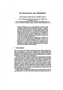
The pLTSs of BB84 and BB84spe for the special case of n = 2 can be depicted as in Figure 2, where for ˜a = K ˜ a = 00. Each arrow in the graph denotes a sequence of simplicity, we only specify the branch where B τ actions, and all probabilistic distributions are uniform. The strings at the bottom line are the outputs of the protocol. Then it can be easily checked from the pLTSs that BB84 ≈o BB84spe . The key is, for each ˜ b line), the final states are bisimilar; they extra branch in BB84 caused by the measurement of Bob (the K all output the same string. The second choice is to use logic formulae. Let T estBB84

def

=

˜ a′ .keyb ?K ˜ b′ . (BB84kkeya?K ˜′ = K ˜ ′ then suc!0.nil else f ail!0))\{keya, keyb }, (if K b a

and ψp = hsuc!0itrue ∧ ¬hτ i(p · hf ail!0itrue + (1 − p) · true) V where true is the abbreviation of i∈∅ φi . It is not difficult to show T estBB84 |= ψp for any p > 0.

20

Now we proceed to describe the protocol where an eavesdropper can be detected. Alice′

def

=

˜ ′ .P str ˜ ′ [˜ ˜′,x ˜ ′′ (Alicekkeya?K ˜].a2b!˜ x.a2b!SubStr(K a a ˜).b2a?Kb . |K | qa ; x a

˜ a′ , x ˜ b′′ then keya′ !RemStr(K ˜ a′ , x (if SubStr(K ˜) = K ˜).nil else alarma !0.nil)))\{keya } Bob′

def

=

˜ ′ .a2b?˜ ˜ ′′ .b2a!SubStr(K ˜ ′, x (Bobkkeyb ?K x.a2b?K b a b ˜). ′ ′′ ′ ˜ ,x ˜ then key !RemStr(K ˜ ′, x (if SubStr(K ˜) = K ˜).nil b

a

b

b

else alarmb !0.nil))\{keyb } BB84′

def

=

Alice′ kBob′

˜ a′ , x ˜ a′ at the indexes specified where |˜ x| is the size of x ˜, the function SubStr(K ˜) returns the substring of K ′ ′ ˜ ˜ ˜′,x by x˜, and RemStr(Ka , x˜) returns the remaining substring of Ka by deleting SubStr(K a ˜). The special measurement P strm , which is similar to Ran, randomly generates a ⌈m/2⌉-sized string of indexes from 1, . . . , m. For the capacity of a potential eavesdropper Eve, we assume that she has complete control of the quantum channel, but can only listen on the classical channels between Alice and Bob. That is, she can do any quantum operations on the communicated qubits from Alice and Bob, one of the extreme cases being keeping the qubits from Alice while creating and sending to Bob some fresh ones, with the same size, prepared by herself. But for classical communication, Eve can only copy and resend the bits without altering them, since Alice and Bob can choose to send them through a broadcasting channel. Note that perfect copying of the qubits transmitted through the quantum channel from Alice to Bob is prohibited by the basic laws of quantum mechanics, since the potential quantum states sent, |0i, |1i, |+i, and |−i in this protocol, are nonorthogonal. With these natural assumptions, an eavesdropper Eve can be described as: Eve ˜ e) W aitE(K

def

n ˜ e ].E2B!˜ ˜ e) A2E?˜ q .E[˜ q ′′ , q˜].M0,1 [˜ q ′′ ; K q .W aitE(K

def

˜b .e2a!B ˜b .a2e?B ˜a .e2b!B ˜ a .a2e?˜ b2e?B x.e2b!˜ x. ′′ ′′ ′′ ′′ ′ ˜ .e2b!K ˜ .b2e?K ˜ .e2a!K ˜ .key !gkey(K ˜ e, B ˜e , B ˜a , B ˜b , K ˜ ′′ , K ˜ ′′ , x a2e?K ˜).nil

=

=

a

a

b

b

e

a

b

where E is a super-operator, and gkey is the function Eve used to generate her guess of the key from the classical information transmitted between Alice and Bob. Then a practical running BB84 protocol, with the existence of an eavesdropper, goes as follows BB84E

def

=

(Alice′ [fa ]kEvekBob′ [fb ])\{a2e, b2e, e2a, e2b, A2E, E2B}

where fa and fb are relabelling functions such that fa (a2b) = a2e, fa (b2a) = e2a, fa (A2B) = A2E, and fb (a2b) = e2b, fb (b2a) = b2e, fb (A2B) = E2B. To get a taste of the security of BB84′ , we consider a special case where Eve’s strategy is to simply measure the qubits sent by Alice, according to randomly guessed bases, to get the keys. She then prepares and sends to Bob a fresh sequence of qubits, employing the same method Alice used to encode keys, but using her own guess of bases and the keys she obtained. That is, we define Eve′

def

=

˜ e) ˜ ˜e ].M ˜ [˜ q ].E2B!˜ q .W aitE(K q ].HB˜e [˜ A2E?˜ q .Ran[˜ q ′′ ; B ˜ e [˜ Be q ; Ke ].SetK

Now let BB84′E be the protocol obtained from BB84E by replacing Eve by Eve′ , and letting the function gkey simply return its first parameter. Let T estBB84′

def

=

(BB84′E kkeya′ ?˜ x.keyb′ ?˜ y .keye′ ?˜ z .(if x ˜ 6= y˜ then f ail!0.nil

else keye !˜ z .skey!˜ x.nil))\{keya′ , keyb′ , keye′ }.

21

It is generally very complicated to prove the security of the full BB84 protocol, even for the simplified Eve′ presented above. Here we choose to reduce T estBB84′ to a simpler process which is easier for further verification. To be specific, we can show that T estBB84′ is bisimilar to the following process: TB

def

=

˜ e ].Ran[˜ ˜b ]. ˜a ].Ran[˜ ˜ a ].Ran[˜ ˜e ].Ran′˜ ˜ ˜ [˜ q; K q′ ; B Ran[˜ q; B q; K q ′′ ; B Ba ,Be ,Ka Ran′B˜e ,B˜

˜

b ,Ke

˜ b ].P str ˜ [˜ [˜ q; K ˜]. |Kab | qa ; x

˜ ab = K ˜ ba then keye !K ˜ e .skey!RemStr(K ˜ ab , x (if K ˜).nil x ˜ x ˜ ˜ ˜ else (if Kab 6= Kba then alarma !0.nilkalarmb !0.nil else f ail!0.nil))

˜ ab = cmp(K ˜ a, B ˜a , B ˜b ), K ˜ ba = cmp(K ˜ b, B ˜a , B ˜b ), K ˜ x˜ = SubStr(K ˜ ab , x ˜), where to ease the notations, we let K ab x ˜ ′ ˜ ˜ and Kba = SubStr(Kba , x ˜). Similar to Ran, the special measurement Ran here, which takes three param˜ e ] will first generate a string of n − |K ˜ ae | q; K eters, delivers a string of n bits. For example, RanB˜a ,B˜e ,K˜ a [˜ ˜ a at the positions where B ˜a and B ˜e do not match, and store random bits x˜, replace with x ˜ the substring of K ˜ e. the string after the replacement in K

7

Conclusion and related work

In our opinion, bisimulations should be considered as a proof methodology for demonstrating behavioural equivalence between systems, rather than providing the definition of the extensional behavioural equivalence itself. We have adapted the well-known reduction barbed congruence used for a variety of process calculi [20, 32, 11, 5], to obtain a touchstone extensional behavioural equivalence for quantum processes considered in [10]. In the literature there are also minor variations on the formulation of reduction barbed congruence, often called contextual equivalence or barbed congruence. See [11, 35] for a discussion of the differences. We have defined a notion of open bisimulations, which provides both a sound and complete coinductive proof methodology for establishing the equivalence between qCCS processes. The operational semantics of this language is given in terms of probabilistic labelled transition systems. Moreover, we have generalised Hennessy-Milner logic to express the behaviour of quantum processes. In the resulting quantum logic, logical equivalence coincides with open bisimilarity. To conclude this paper, we would like to compare the open bisimulation defined here with other bisimulations for quantum processes already proposed in the literature. Jorrand and Lalire [25, 27] defined a branching bisimulation for their QPAlg, which identifies quantum processes whose associated graphs have the same branching structure. However, their bisimulation cannot always distinguish different quantum operations, as quantum states are only compared when they are input or output. More seriously, the derived bisimilarity is not a congruence; it is not preserved by restriction. Bisimulation defined in [9] indeed distinguishes different quantum operations but it works well only for finite processes, since quantum states are compared after all actions have been performed. Again, it is not preserved by restriction, and whether it is preserved by parallel composition still remains open, although the positive answer is affirmed in two special cases. In [41], a congruent (strong) bisimulation was proposed for a special model where no classical datum is involved. However, as many important quantum communication protocols such as superdense coding and teleportation cannot be described in that model, the scope of its application is very limited. Furthermore, as all quantum operations are regarded as visible in [41], the bisimulation is too strong; it distinguishes two different sequences of quantum operations even when they have the same effect as a whole. The first general (works for general models where both classical and quantum data are involved, and recursive definition is allowed), weak (quantum operations are regarded as invisible, so that they can be combined arbitrarily), and congruent bisimulation for quantum processes was defined in [10]. It differentiates quantum input, to match which an arbitrarily chosen super-operator should be considered, from other actions. The open bisimulation in this paper makes a step further by treating the super-operator application in an ‘open’ style: applying super-operators before an action to be matched is selected. This makes it possible to 22

separate ground bisimulation and the closedness under super-operator application, and by doing so, we are able to provide not only a neater and simpler definition, but also a powerful technique for proving bisimilarity. It is easy to prove that the bisimulation in [10] is both a ground bisimulation and closed under superoperator application. Then by Proposition 5.5, it is also an open bisimulation; in other words, the bisimilarity presented in the current paper is coarser than that defined in [10]. Whether or not they are actually the same is an interesting question, and we leave it for further investigation.

References [1] Jos C. M. Baeten and W. P. Weijland. Process Algebra, volume 18 of Cambridge Tracts in Theoretical Computer Science. Cambridge University Press, 1990. [2] C. H. Bennett and G. Brassard. Quantum cryptography: Public-key distribution and coin tossing. In Proceedings of the IEEE International Conference on Computer, Systems and Signal Processing, pages 175–179, 1984. [3] C.H. Bennett, G. Brassard, C. Crepeau, R. Jozsa, A. Peres, and W. Wootters. Teleporting an unknown quantum state via dual classical and EPR channels. Physical Review Letters, 70:1895–1899, 1993. [4] C.H. Bennett and S.J. Wiesner. Communication via one- and two-particle operators on EinsteinPodolsky-Rosen states. Physical Review Letters, 69(20):2881–2884, 1992. [5] Yuxin Deng and Matthew Hennessy. On the semantics of markov automata. In Proceedings of the 38th International Colloquium on Automata, Languages and Programming, volume 6756 of Lecture Notes in Computer Science, pages 307–318. Springer, 2011. [6] Yuxin Deng and Catuscia Palamidessi. Axiomatizations for probabilistic finite-state behaviors. Theoretical Computer Science, 373(1-2):92–114, 2007. [7] Yuxin Deng, Rob van Glabbeek, Matthew Hennessy, and Carroll Morgan. Testing finitary probabilistic processes (extended abstract). In Proceedings of the 20th International Conference on Concurrency Theory, volume 5710 of Lecture Notes in Computer Science, pages 274–288. Springer, 2009. [8] Yuxin Deng, Rob van Glabbeek, Carroll Morgan, and Chenyi Zhang. Scalar outcomes suffice for finitary probabilistic testing. In Proceedings of the 16th European Symposium on Programming, volume 4421 of Lecture Notes in Computer Science, pages 363–378. Springer, 2007. [9] Y Feng, R Duan, Z Ji, and M Ying. Probabilistic bisimulations for quantum processes. Information and Computation, 205(11):1608–1639, 2007. [10] Yuan Feng, Runyao Duan, and Mingsheng Ying. Bisimulation for quantum processes. In Proceedings of the 38th ACM SIGPLAN-SIGACT Symposium on Principles of Programming Languages, pages 523– 534. ACM, 2011. [11] C´edric Fournet and Georges Gonthier. A hierarchy of equivalences for asynchronous calculi. Journal of Logic and Algebraic Programming, 63(1):131–173, 2005. [12] S. J. Gay and R. Nagarajan. Communicating quantum processes. In J. Palsberg and M. Abadi, editors, Proceedings of the 32nd ACM SIGPLAN-SIGACT Symposium on Principles of Programming Languages (POPL), pages 145–157, 2005. [13] SJ Gay and R Nagarajan. Types and typechecking for communicating quantum processes. Mathematical Structures in Computer Science, 16(03):375–406, 2006. [14] L. K. Grover. A fast quantum mechanical algorithm for database search. In Proc. ACM STOC, pages 212–219, 1996. 23

[15] L. K. Grover. Quantum mechanics helps in searching for a needle in a haystack. Physical Review Letters, 78(2):325, 1997. [16] M. Hennessy. A proof system for communicating processes with value-passing. Formal Aspects of Computer Science, 3:346–366, 1991. [17] M. Hennessy and A. Ing´olfsd´ottir. A theory of communicating processes value-passing. Information and Computation, 107(2):202–236, 1993. [18] Matthew Hennessy and Robin Milner. Algebraic laws for nondeterminism and concurrency. Journal of the ACM, 32(1):137–161, 1985. [19] C. A. R. Hoare. Communicating Sequential Processes. Prentice Hall, 1985. [20] Kohei Honda and Mario Tokoro. On asynchronous communication semantics. In P. Wegner M. Tokoro, O. Nierstrasz, editor, Proceedings of the ECOOP ’91 Workshop on Object-Based Concurrent Computing, volume 612 of LNCS 612. Springer-Verlag, 1992. [21] A. Jeffrey and J. Rathke. Contextual equivalence for higher-order pi-calculus revisited. Logical Methods in Computer Science, 1(1:4), 2005. [22] Bengt Jonsson, C. Ho-Stuart, and Wang Yi. Testing and refinement for nondeterministic and probabilistic processes. In Proceedings of the 3rd International Symposium on Formal Techniques in Real-Time and Fault-Tolerant Systems, volume 863 of Lecture Notes in Computer Science, pages 418–430. Springer, 1994. [23] Bengt Jonsson and Wang Yi. Compositional testing preorders for probabilistic processes. In Proceedings of the 10th Annual IEEE Symposium on Logic in Computer Science, pages 431–441. Computer Society Press, 1995. [24] Bengt Jonsson and Wang Yi. Testing preorders for probabilistic processes can be characterized by simulations. Theoretical Computer Science, 282(1):33–51, 2002. [25] P. Jorrand and M. Lalire. Toward a quantum process algebra. In P. Selinger, editor, Proceedings of the 2nd International Workshop on Quantum Programming Languages, 2004, page 111, 2004. [26] K. Kraus. States, Effects and Operations: Fundamental Notions of Quantum Theory. Springer, 1983. [27] Marie Lalire. Relations among quantum processes: Bisimilarity and congruence. Mathematical Structures in Computer Science, 16(3):407–428, 2006. [28] R. Milner. Communication and Concurrency. Prentice-Hall, 1989. [29] R. Milner, J. Parrow, and D. Walker. A calculus of mobile processes, parts i and ii. Information and Computation, 100:1–77, 1992. [30] M. Nielsen and I. Chuang. Quantum computation and quantum information. Cambridge univer- sity press, 2000. [31] Martin L. Puterman. Markov Decision Processes. Wiley, 1994. [32] Julian Rathke and Pawel Sobocinski. Deriving structural labelled transitions for mobile ambients. In Proceedings of the 19th International Conference on Concurrency Theory, volume 5201 of Lecture Notes in Computer Science, pages 462–476. Springer, 2008. [33] Julian Rathke and Pawel Sobocinski. Making the unobservable, unobservable. Electronic Notes in Computer Science, 229(3):131–144, 2009.

24

[34] D. Sangiorgi, N. Kobayashi, and E. Sumii. Environmental bisimulations for higher-order languages. In Proceedings of the 22nd IEEE Symposium on Logic in Computer Science, pages 293–302. IEEE Computer Society, 2007. [35] D. Sangiorgi and D. Walker. The π-calculus: a Theory of Mobile Processes. Cambridge University Press, 2001. [36] Davide Sangiorgi. A theory of bisimulation for the pi-calculus. Acta Informatica, 33(1):69–97, 1996. [37] Roberto Segala. Modeling and verification of randomized distributed real-time systems. Technical Report MIT/LCS/TR-676, PhD thesis, MIT, Dept. of EECS, 1995. [38] Roberto Segala and Nancy A. Lynch. Probabilistic simulations for probabilistic processes. Nordic Journal of Computing, 2(2):250–273, 1995. [39] P. W. Shor. Algorithms for quantum computation: discrete log and factoring. In Proceedings of the 35th IEEE FOCS, pages 124–134, 1994. [40] J. von Neumann. States, Effects and Operations: Fundamental Notions of Quantum Theory. Princeton University Press, 1955. [41] M Ying, Y Feng, R Duan, and Z Ji. An algebra of quantum processes. ACM Transactions on Computational Logic (TOCL), 10(3):1–36, 2009.

25