their outputs by using a kernel-based regression to effectively combine them into a single detector. This study ... the Royal Norwegian Navy. The sensor used is ... Bay of La Spezia where several realistic dummy mine targets were deployed. 2.
Proceedings of the Institute of Acoustics
FUSION OF CONTACTS IN SYNTHETIC APERTURE SONAR IMAGERY USING PERFORMANCE ESTIMATES †
Vincent Myers Øivind Midtgaard
1
NATO Undersea Research Centre, La Spezia Italy. Norwegian Defence Research Establishment (FFI), Kjeller, Norway.
INTRODUCTION
Automatic Target Recognition (ATR) enables mine countermeasures (MCM) using autonomous underwater vehicles (AUVs). ATR makes non-trivial autonomy feasible by providing information which allows making choices about mission parameters in real time and relying less on human intervention. It also supports networking by on-board decision making to make intelligent use of the limited communications bandwidth underwater. ATR is typically divided into two stages: detection, which is the process of determining the presence of target signatures in a sonar image, and classification, during which a more refined discrimination 1 is performed . Detection is arguably the most vital step in any automatic target recognition (ATR) system. Without a reliable detection method, the system performance degrades as any further discrimination becomes impossible since only detected objects are afforded the chance to be further processed by any subsequent steps. The application of combining multiple detection algorithms is 2 widespread. For instance Casasent and Ye fused the output of two algorithms to detect objects in infrared images by using a logical “and” method. Fusion of multiple detection algorithms has also 3 been applied to the classification of underwater objects using sonar images; for instance, Dobeck fuses the output of three classifiers by way of a Fisher Discriminant which uses the normalized confidences of the individual detectors as well as the possible combinations of detectors. Aridgides 4 fuses the same three algorithms using a number of logical operators as well as a log likelihood 5 ratio test. Reed et al. applied Dempster-Shafer theory to the fusion of multiple views of the same object in order to increase the overall classification performance; similar methods were also 6 7 proposed earlier by Stage and Zerr . Fawcett implemented several simple detectors and fused their outputs by using a kernel-based regression to effectively combine them into a single detector. This study concentrates on the detection stage of the ATR process, with particular emphasis on the combination of multiple detection algorithms. A through-the-sensor method for assessing detector performance is first presented. The evaluation is done by simulating synthetic aperture sonar (SAS) target signatures and embedding them with the real mission data. Sensor performance is assessed using a sonar performance prediction tool and signatures are generated using a ray tracing method. The detector performance is then assessed on the simulated targets and used for fusing four simple detection methods using Dempster-Shafer theory of evidence, which includes a methodology incorporating information provided by missed detections. The method is tested on a dataset of SAS imagery obtained during sea experiments conducted by the NATO Undersea Research Center, the Norwegian Defence Research Establishment (FFI) and the Royal Norwegian Navy. The sensor used is the Edgetech 4400 SAS mounted on the HUGIN 8 1000 autonomous underwater vehicle (AUV) which was used in two separate mission areas in the Bay of La Spezia where several realistic dummy mine targets were deployed.
2
DETECTORS 7
Four detectors are used in this study and are very similar to those described by Fawcett . All of these detectors operate by computing statistics in a window based on a template of a generic target †
The author is currently with Defence Research and Development Canada – Atlantic, Halifax, Canada.
Vol. 29. Pt.6 2007
Proceedings of the Institute of Acoustics
signature. Since the geometry of side-looking sonar is such that the expected size of target signature will change according to the range of the object, the detector window sizes are adjusted in the across-track direction based on the image resolution.
2.1 Matched filter 9
The matched filter is one of the most commonly used detection algorithms. It operates on the principle of the correlating image data with an idealized target signature, in this case an area of bright pixels (the target echo) followed shortly by an area of dark pixels (the shadow) of the expected size. In this implementation, the image is first normalized by dividing each image pixel at range r by the mean pixel value in the image at that range, and then de-medianed (thus dark pixels receive negative values). A 2D convolution is performed with a rectangular mask representing a “generic” target signature containing +1 in the echo zone and -1 in the expected shadow zone. A high output indicates a high degree of correlation of the data with the idealized mine mask.
2.2 Lacunarity The lacunarity
10
of an area of pixels is defined as
=
σ2 µ2
,
(1)
where σ2 is the pixel variance and μ is the mean of the pixel amplitudes. This metric produces high output when the variance with an area is large compared to its mean and was originally devised to discriminate between man-made and natural objects based on shadow statistics. As a detection algorithm, Equation (1) is computed for an expected shadow-sized window, adapted for range.
2.3
Segmented matched filter 9
This method is a variation on the matched filter method ; however a more refined segmentation is performed beforehand. Based on the median pixel amplitude ( ~ x r ), which is computed as a function of the range r to remove beampattern effects, an image segmented as follows: pixels at range r less than 0.3 ~ x r are assigned -0.5 (shadow), pixels x r are assigned -1 (deep shadow), less than 0.6 ~
greater than 2 ~ x r are assigned +0.5 (highlights) and finally those greater than 4 ~ x r are assigned 1 (bright highlights). To reduce the large numbers of false alarms caused by extended highlight and shadows which extend past the filter window, the image I is normalized as follows:
IN =
I , 1 + 10 N
(2)
where N is the average value of the segmented image over a larger window surrounding the targetsized matched filter window. This normalization penalizes the score and reduces the number of false alarms due to extended objects of fields of sand ripples.
2.4 Mean test ‡
The final detector is a test on the means based on a statistical Z-test , where the standard error is replaced by the standard deviation, resulting in:
z=
µ1 − µ 2 σ2
,
(3)
where μ1 and μ2 are the computed means within highlight and shadow windows comparable to the idealized target signature matched filter described above and σ2 is the standard deviation in the area corresponding to the shadow area. This detector will generate high values of z when a bright region is followed by a darker, homogenous region, such as the signature produced by a proud target.
‡
This detector was devised by Y. Petillot of Heriot-Watt University, Edinburgh, Scotland.
Vol. 29. Pt.6 2007
Proceedings of the Institute of Acoustics
Figure 1. ESPRESSO predictions for highlights, shadows and backgrounds for the Edgetech sensor in approx. 30 m water depth and 14 m altitude. The seabed was composed of silty mud and the wind speed was low.
3
FAST SIMULATION OF SAS TARGETS
The fusion method developed in this paper requires that the performance of the detector be either known or somehow estimated. To arrive at such an estimate, a strategy involving the simulation of 11,12 . The target signatures and inserting them into the mission sonar imagery is applied performance of the detectors can then be evaluated in a controlled manner with the ground truth at hand. The method used to simulate the required target signatures uses ray tracing combined with a sonar performance prediction tool to generate a probabilistic representation of a target, which is then blended into the mission imagery. 13,14,15
. For the High-frequency target modelling has been a topic of research for many years methodology described here to be useful, the statistical determination of detector performance must be done on-line, which therefore requires that signatures be generated quickly. Less importance is put on modelling seabed reverberation, for instance, since the mission data will be used as background texture. This fusion of simulated targets with mission data has been proposed by 16,17 who developed a method for adding target signatures to sonar imagery using an Coiras et al. 18 inversion technique. Putney et al. employed a physics-based approach to the modelling by using acoustic ray tracing, resulting in greater realism for the target signatures. The targets capable of being modelled are required to have a mathematical description (cylinders, spheres). The method described here uses simple optical ray tracing combined with a sonar performance prediction tool to produce target signatures capable of being used as prediction methods for the detectors.
3.1 Ray tracing For high-frequencies (≥ 100 kHz), ray tracing is the most widely used method due mainly to the high computational burden of other methods (finite elements, normal modes, etc…). While ray theory permits direct calculation of range and time of returns, it is not able to describe wave effects such as diffraction and usually results in unnaturally crisp shadow zones. The target is described as a set of interconnected triangular facets designed using a computer program. Rather than compute acoustic scattering from the target this method is concerned with determining mean highlight, background and shadow zone using principles of geometric optics. Once a minimum travel time and corresponding grazing angle for a ray is found, it is simple to verify whether it has intersected the seabed or the target. If it intersects the target then a normalized value of 1 times the sine of the grazing angle scaled by the directivity of the ray is used as a return. After a series of rays has been traced, the times are sorted in ascending order and interpolated at a spacing equivalent to the sampling frequency of the beamformed image with returns occurring at
Vol. 29. Pt.6 2007
Proceedings of the Institute of Acoustics
13
the same time being summed together, based on the method by Bell . No returns for a given time step results in a shadow zone. The result of the ray-tracing step is a proportional map of shadow, echo and seabed pixel values. Since scattering, and therefore acoustic pressure, is not directly computed, some method of computing reasonable pixel amplitudes is required.
3.2 ESPRESSO ESPRESSO is a sonar modelling tool capable of modelling the acoustic sound field. Reverberation 19 is calculated using geometrical beam tracing , which approximates the seabed sea surface and volume as lines of scatterers, which results in a reverberation time series. A bistatic seabed scattering as well as reflection loss models are taken from the acoustic models developed by the 20 Applied Physics Laboratory . The ESPRESSO tool takes parameters such as sensor design characteristics as well as environmental parameters to produce predicted shadow to background Sonar images are obtained following a series of processing steps and can rarely be brought back to acoustic pressure. Analogue to digital conversion, frequency filters and time varying gain are some examples of processing which become difficult to reverse. Therefore, while the predictions are accurate enough for the purposes herein, the values need to be transformed into values which are in line with the image under consideration. To accomplish this, the shadow and echo levels in image gray levels are computed as to maintain the same contrast ratio as the acoustic pressures predicted by ESPRESSO. For a given image, the mean gray level vs. range cell is computed, which serves as the background curve. Going back to the predicted values, the contrast ratios are kept the same versus this mean image gray level. When a target and environment has been modelled, probabilistic pixel amplitudes are generated as per the ESPRESSO predictions. First Rayleigh noise is added to all modelled pixels with a parameter equal to the shadow level for the range of the pixel. This noise represents sensor and reverberation noise, including multipath. Next noise is added to the echo at a level equal to the predicted echo level, scaled by the average grazing angles computed by the ray tracing model. The final step is to fuse the generated target with the sonar imagery. Due to the finite width of the acoustic beam, pixels on the boundary may consist of some proportion of shadow and seabed. During ray tracing, these proportions are computed so that during the combination stage pixels are blended smoothly with appropriate levels of simulated and real data, creating smooth and more realistically blurred shadow boundaries.
Figure 2. Simulated targets from the Edgetech sensor. ESPRESSO predictions for highlight, shadow and background for one of the missions are shown in Figure 1 and simulated target signatures from the Edgetech synthetic aperture sonar used in the study are shown in Figure 2.
Vol. 29. Pt.6 2007
Proceedings of the Institute of Acoustics
3.3 SAS issues The model described above was developed to simulate targets using a planar array. With synthetic aperture sonar, however, several array lengths are combined along the sensor travel path to create an effective array of some length longer than the original. In order for the simulation method to generate realistic SAS target signatures, the imagery must be simulated using the effective synthetic array length. This effective length changes with the range r. The theoretical SAS gain, QSAS is equal to:
Q SAS =
2λ r , LT LR
(4)
where λ is the wavelength of transmitted signal and LT and LR are the lengths of the transmit and receive arrays. This follows from the ratio of the physical resolution of the array λr / LR and the 21
theoretical SAS resolution LT / 2 . Therefore, the resulting beam pattern for a receive array of n elements focusing at a range of r is simulated as one having n times QSAS elements, effectively creating a synthetic aperture at range r.
4
DETECTOR PERFORMANCE
The next step is to determine the detector performance characteristics by using the simulated signatures generated above. Two parameters are required for the fusion algorithm: a measure of detector confidence and the probability of detection versus range.
4.1 Detector Confidence The confidence of a detection is used to assign values to the mass function when fusing detections with Dempster-Shafer theory, which is described in Section 5. The detection of targets is achieved by thresholding the output of the detection algorithm over the mission sonar imagery. Some filtering is done on the size of the detections to remove contacts which are too small or large. Once found, determination of the likelihood of this detection must be made in order to assign a belief to the hypothesis that the contact is in fact a legitimate one. These likelihood functions are constructed using the simulated target data generated from the signature modelling method described above. A dataset of images is chosen to estimate this performance. Several iterations of simulation followed by the application of the detectors are performed. Let γ T be the output of the detector over a given SAS image without simulated targets and γ T be the response on the same image with a number simulated target signatures. Since the images differ only at the pixels where the targets were added, the conditional probability of a detector’s response to a target signature can be estimated using: (5) p (γ | T) = H (γ T ),
Vol. 29. Pt.6 2007
Proceedings of the Institute of Acoustics
Figure 3. Confidence of the matched filter detector as a function of the output γ for three different threshold values. where H(γT) is the normalized histogram of the detector output over the simulated targets. A similar method is used to estimate the probability density function for the non-target class. Bayes’ theorem is applied to obtain the conditional probability of a target given a threshold:
P (T | γ > τ ) = where
P(γ > τ | T) P(T) , P(γ > τ | T) P(T) + P(γ > τ | T) P(T)
(6)
P(T) is the prior probability of a target and ∞
P(γ > τ | T) = ∫ p (γ | T)dγ ,
(7)
τ
where P (T ) = 1 − P (T ) . The overall choice of P (T ) seemed to have minor effects on the fusion scheme described in the results section, and was arbitrarily set to 0.1. Equation (6) is the confidence value used in the fusion method and it depends on the threshold as described in Equation (7). This dependency has the consequence that is it possible that two objects detected at the same γ using different thresholds τ1 and τ2 (where γ > τ1, τ2) will result in different confidence values. Figure 3 shows how the confidence of the matched filter detector is changed depending on the threshold used.
4.2 Detection performance versus range Another performance metric required is the probability of detection versus range for a given detector, commonly called a P(y) curve. Since the target signatures are simulated at known positions in the image, it is simple to determine the P(y) performance of a detector. By keeping track of the signature generation ranges, then for a given threshold τ the P(y) at range r is simply the ratio between the number of targets detected and the number of targets generated. These curves for the detection algorithms as well as for the thresholds used in Section 6 are shown in Figure 4.
Vol. 29. Pt.6 2007
Proceedings of the Institute of Acoustics
Figure 4. P(y) curves for all detectors for a fixed threshold.
5
DEMPSTER-SHAFER FUSION
Once the detector confidence values and P(y) curves have been determined, it is possible to devise a method for fusing the results using the Dempster-Shafer theory of evidence (DSTE), which is a mathematical formalism for assigning and combining the belief when that belief is due to evidence 22 from independent sources . A very brief outline of DSTE is given here. Suppose an observation can be explained by one of a finite set of n mutually exclusive and exhaustive hypotheses. This set is called the frame of discernment and denoted Θ={H1,H2,..,Hn}. Each hypothesis Hi⊂Θ corresponds to a one-element subset {Hi}, called a focal element. A composite hypothesis denoting the disjunction Hi ∪ .. ∪ Hj is represented by the subset {Hi,..,Hj }⊂Θ. The collection of all possible subsets of Θ (including the empty set Ø and Θ itself) is called the is Θ denoted 2 . Based on evidence such as an observation, DSTE assigns corresponding beliefs in the n range [0..1] to all 2 elements in the power set. Belief is distributed through a basic probability assignment (BPA), called a mass function, which is a mapping from the power set to the unit interval, m: 2Θ → [0, 1], satisfying:
m(Ø) = 0
∑ m( A) = 1,
(8)
A⊆Θ
This basic probability assignment m(A), represents the portion of belief committed exactly to A and not to any subsets B of A. The extent to which the evidence specifically supports belief in the hypothesis represented A (i.e. the total belief in A), is given by a belief function which is the sum of all basic probability values m(B) in all subsets of A:
Bel ( A) =
∑ m( B),
(9)
B⊆ A
Mass functions of two sets B, C on the same frame of discernment from independent sources can be combined provided they are not totally contradictory. The orthogonal sum m of two mass functions m1 and m2 is denoted by m= m1 ⊕ m2 yields a basic probability assignment and is given by Dempster’s rule of combination: m(Ø) = 0
m( A) = provided that:
Vol. 29. Pt.6 2007
∑ 1− ∑
B ∩C = A
m1 ( B)m2 (C )
B ∩C = Ø
m1 ( B)m2 (C )
,
(10)
Proceedings of the Institute of Acoustics
∑ m ( B)m
B ∩C = Ø
1
2
(C ) < 1,
(11)
23
During an MCM mission , one (or perhaps several) sensors are used to image the seafloor in the area. Depending on the survey line pattern, sensor range and view-angles, each sensor may cover a given seafloor position zero, one or multiple times. The hypotheses under consideration are: Hypothesis T : There is a target at position (x,y). Hypothesis
T : There is not a target at position (x,y).
During a mission, when the output of one of the automatic algorithms exceeds the chosen threshold τ, this results in a detection. Evidence supporting the hypothesis that a target is present is assigned using Equation (6): m(T ) = P(T |γ > τ ) , (12) where γ is the maximum detector output for the cluster of pixels which exceeded τ. When detector i detects a target, one of two events may occur with respect to another detector j: Either detector j will also detect a target at the same location as detector i, or detector j will not exceed its threshold value and will therefore not detect a target a the given location. In the first case of a corresponding detection, additional evidence supporting hypothesis T is assigned using Equation (12) according to its own confidence value computed using Equation (6). In the second case, the evidence supports the hypothesis that a target is not present at this location; therefore hypothesis T is supported to a degree that is equal to the performance of the detector at range r, the distance from the location to the position of the sensor:
m(T) = Pd (r ) ,
(13)
where Pd(r) is the probability of detection of detector d at range r. If a detector performs well at range r, then a non-detection highly supports the hypothesis T ; if the detector performs poorly, then there is less support for T . Note that the second case does not directly result in evidence for T. Since survey tracks are usually designed to cover the same area more than once, there may be many opportunities to detect a target at a given location. The same strategy as above can be applied to detections from overlapping tracks: In the case of coinciding detections, evidence is assigned to hypothesis T according to a detector’s confidence curves; when detections are missing, the range to the sensor is computed and evidence supporting hypothesis T is assigned according the P(y) curve of the detector in question. For an associated group of detections and possibly missing detections, the set of basic probability assignments are fused through iterative use of Dempster’s rule of combination: m = m1 ⊕ m2 ⊕ … ⊕ mk for k pieces of evidence. A belief in hypothesis T (and T ) for each group position is finally obtained using Equation (9).
6
RESULTS
The detection and fusion method was tested on two data sets obtained during collaborative sea trials between FFI, the Norwegian Navy and the NATO Undersea Research Centre in La Spezia, 24 25 Italy, namely MX3 and SWIFT which took place between October and December 2005. A total of 16 dummy targets were deployed including truncated cone, wedge and cylinder shapes. The HUGIN 1000 Autonomous Underwater Vehicle equipped with a high-grade inertial navigation system and the Edgetech 4400 SAS-capable sonar was used to perform multiple surveys of the area. This sensor operates at a centre frequency of 120 kHz and is capable of obtaining a theoretical image resolution of 10 cm square. Two missions have been analyzed, one from 01/12/05 over 8 targets in the SWIFT trials area and one from 16/11/05 in the MX3 experiments. The vehicle tracks and target deployment positions are shown in Figure 5.
Vol. 29. Pt.6 2007
Proceedings of the Institute of Acoustics
A random SAS image was chosen from the available data set to estimate the detector confidence and P(y) curves. A mix of 40 synthetic targets was generated in the image, repeated over 50 iterations, resulting in a total of 2000 target signatures.
Figure 5 SWIFT and MX3 operational areas. Target fields are shown, as well as HUGIN 1000 vehicle tracks and area coverage. Figure 6(a) shows the results of processing to obtain ROC curves for each individual detector on the 26 two mission datasets. Dobeck suggested that robust fusion can be performed when adjusting the detector thresholds such that the minimum number of false alarms is obtained for a probability of detection equal to one. Here, the real targets are used to compute these ROC curves in order to obtain the best thresholds for the method. Three of the detectors are able to obtain a 100 % probability of detection and the corresponding operating point used for the fusion is shown. The fourth detector (the matched filter) however, is unable to attain such a high detection probability, with an ROC curve flattening out at Pd = 0.79. Therefore the operating point which gives the least false alarms for this maximum performance is chosen to fuse this detection method. Figure 6(b) shows the performance of the DSTE fusion methodology described above for the chosen detector thresholds. By thresholding the belief of the Dempster-Shafer fusion result, it is possible to obtain ROC curves for a given mission. Several curves are shown: First, the dotted line shows results of fusion using only the three best detectors without the matched filter (MF) and without incorporating the information gained by missing detections from multiple passes. Next, by adding information provided by non detections in different legs, the solid line is obtained. Finally, by the adding the MF detector, whose performance is not at the level of the other three, the dash-dot line is obtained. Note that this ROC curve is slightly better than the one obtained without the MF § algorithm , but what is interesting is that the performance is not degraded. This is due to the fact that the confidence of this detector is lower and therefore the DSTE fusion method is robust to its poor performance. Also, the square shows the performance of “and”-ing the three best detectors, which results, as predicted by Dobeck, in a significant reduction in false alarms and an operating point similar to the ROC curve obtained without incorporating missed detections. The triangle shows the result of “and”-ing all four detectors. Since the MF detector implementation here does not achieve high detection rates, the performance is set to the worst of all the four detectors. Although for the given false alarm rate it appears to be slightly better than the other methods and individual detectors it is key to note that this is the maximum performance for this fusion method. Also shown is the result of “or”-ing the four detectors, resulting in very high numbers of false alarms. For these results the thresholds were obtained using the real target data in order to fairly compare the proposed fusion method to other methods. In practice, obtaining the thresholds in this way would require a training set, although it should be possible to use the synthetic target signatures
§
Although perhaps not significantly so
Vol. 29. Pt.6 2007
Proceedings of the Institute of Acoustics
that were used to estimate confidence and P(y) performance to also provide the thresholds such as those that were calculated with real targets shown in Fig. 7(a).
(a)
(b)
Figure 6 Results of fusion for (a) the four individual detection methods and (b) the fusion schemes. The probability of detection is plotted versus the total number of false alarms.
7
CONCLUSIONS
This paper has described a methodology to fuse four simple target detection algorithms using the Dempster-Shafer theory of evidence. The basic probability assignments for the fusion are obtained using a strategy whereby target signatures are simulated and the output of the detectors is used to estimate confidence values. The environment and target characteristics are taken into account using a sonar performance prediction tool. These confidence values are directly used to assign belief to the target hypothesis used during the fusion. Information from missed detections is also used by assigning belief to the non-target hypothesis based on the P(y) curves of the detectors, which are also computed during the modelling stage. The fusion method was demonstrated on data from two missions where the Edgetech 4400 synthetic aperture sonar (SAS) was mounted on the HUGIN 1000 AUV. Using three detectors which were able to detect all of the deployed targets, the fusion method without using missed detections achieved results similar to a logical “and”-ing of these methods, with slightly less false alarms. By then incorporating the information provided by missed detections, which in effect takes into account the concept of a sonar “sweet spot” for which performance is better, the resulting false alarm rate outperforms the simple logical operators while maintaining the same detection performance. Then, adding a fourth algorithm which did not perform very well had very little effect on performance of the method and in fact improved it slightly, which shows the robustness of the method to poorly performing detectors. How does this methodology help autonomy? For any autonomy system to be non-trivial, it requires, among other things, an ATR which provides it with useful information on which to base decisions 27 about its dynamic behaviour . The fusion method described here provides two significant elements that can be exploited by an autonomy system, notably reliable confidence and ensuing belief measures, as well as reducin3g the number of false alarms compared with other detection / fusion methods. Using knowledge of the sensor and detector performances will greatly improve the robustness of the ATR system as a whole, and consequently the autonomy.
Vol. 29. Pt.6 2007
Proceedings of the Institute of Acoustics
ACKNOWLEDGEMENTS The authors gratefully acknowledge the work of Karna Bryan, Giampaolo Cimino and Gianfranco Arcieri for their work on the AUV Planning and Evaluation tool, and particularly Gary Davies for help with the ESPRESSO model. Ben Evans was the scientist in charge of the SWIFT trials and Edoardo Bovio was responsible for the organization of the MX3 experiments. Finally, credit is due to John Fawcett, DRDC Atlantic, for his clear and concise work on the detection methods used in this paper.
REFERENCES 1. P.H. Haley and J.E. Gilmour, Two-stage detection and discrimination system for side scan sonar equipment (Westinghouse), US Patent 5,493,539, 1996. 2. D. Casasent and A. Ye, “Detection filters and algorithm fusion for ATR,” IEEE Transactions on Image Processing, vol. 6, no. 1, pp. 114–125, 1997. 3. G. Dobeck, “Algorithm fusion for the detection and classification of sea mines in the very shallow water region using side-scan sonar imagery,” in Proceedings of the SPIE, vol. 4038, pp. 348 – 361, 2000. 4. T. Aridgides, M. Fernandez, and G. Dobeck, “Side scan sonar imagery fusion for sea mine detection and classification in very shallow water,” in Proceedings of the SPIE, vol. 4394, pp. 1123– 1134, 2001. 5. S. Reed, Y. Pettilot, and J. Bell, “Automated approach to classification of mine-like objects in sidescan sonar using highlight and shadow information,” IEE Sonar Radar & Navigation, vol. 151, no. 1, pp. 48–56, 2004. 6. B. Stage and B. Zerr, “Application of the Dempster-Shafer theory to combination of multiple view sonar images,” in UDT ’96 Conference Proceedings, London, UK, 1996. 7. J.A. Fawcett, A. Crawford, D. Hopkin, V. Myers, and B. Zerr, “Computed-aided detection of targets from the CITADEL trial Klein data,” Defence Research and Development Canada, Tech. Rep., 2006. 8. HUGIN website http://www.ffi.no/hugin 9. G. Dobeck, J. Hyland, and L. Smedley, “Automated detection/classification of seamines in sonar imagery,” in Proceedings of the SPIE, vol. 3079, 1997, pp. 90–110. 10. R. Kessel, “Using sonar speckle to identify regions of interest and for mine detection,” Proc. SPIE Vol. 4742, 2002, pp. 440-445. 11. Y. Petillot, S. Reed, and E. Coiras, “A framework for evaluating underwater mine detection and classification algorithms using augmented reality,” in UDT Europe 2006 Conference Proceedings, Hamburg, Germany, 2006. 12. V. Myers, D. Davies, Y. Petillot, and S. Reed, “Planning and evaluation of AUV missions using a data-driven approach,” in Proceedings of the 7th international conference of technology and the mine problem. Montery, Ca: MINWARA, May, 2006. 13. J. Bell, “A model for the simulation of sidescan sonar,” Ph.D. dissertation, Heriot-Watt University, 1995. 14. G. Sammelmann, J. Christoff, and J. Lathrop, “Synthetic images of proud targets,” in OCEANS 94, 1994, pp. 266–271. 15. J.A. Fawcett, “Modeling of high-frequency scattering from objects using a hybrid Kirchoff/diffraction approach,” Journal of the Acoust. Soc. Am. Vol. 109(4), April 2001.
Vol. 29. Pt.6 2007
Proceedings of the Institute of Acoustics
16. E. Coiras, Y. Petillot, and D. Lane, “Multi-resolution 3d reconstruction from side-scan sonar images,” IEEE Transactions on Image Processing, 2007. 17. E. Coiras, P.-Y. Mignotte, Y. Petillot, J. Bell, and K. Lebart, “Supervised target detection and classification by training on augmented reality data,” IEE Proceedings on Radar, Sonar & Navigation, 2006. 18. A. Putney, J. Harbaugh, and M. Nelson, “Target injection for SAS CAD/CAC training and testing,” in Proceedings of the Institute of Acoustics, 2006, pp. 283–290. 19. M. Meyer and G. Davies, “Application of the method of geometric beam tracing for high frequency reverberation modelling,” Acta Acustica, vol. 88, pp. 642–644, 2002. 20. APL-WS, “High-frequency ocean environmental acoustic models handbook,” Applied Physics Laboratory, University of Washington, Tech. Rep. 9407, 1994. 21. L.J. Cutrona, “Comparison of sonar system performance achievable using synthetic aperture techniques with the performance achievable by more conventional means,” Journal of the Acoust. Soc. Am. Vol. 58(8), pp 336-346, 1975. 22. G. Shafer, A Mathematical Theory of Evidence, Princeton University Press, 1976. 23. Ø. Midtgaard, HUGIN MRS – Object Detection Fusion, Tech. Rep. NOTAT-2006/01558, FFI, Norway, 2006. 24. E. Bovio, “Autonomous Underwater Vehicles for scientific and Naval Operations,” in Annual Reviews in Control 25. V. Myers, B. Evans, D. Hopkin, B. Zerr, J.A. Fawcett, A. Crawford, P.E. Hagen, and M. Flores, “The CITADEL and SWIFT joint experiments with unmanned vehicles for minehunting and highfrequency sensors," in Proceedings of the 7th International Conference on Technology and the Mine Problem, 2006. 26. G. Dobeck “On the power of algorithm fusion,” in Proceedings of the SPIE, Vol. 4394, pp 10921102, 2001. 27. B. Evans, “AUV Autonomy: Requirements, approach and system implementation,” Tech. Rep. NATO Undersea Research Centre, Italy, 2007.
Vol. 29. Pt.6 2007