Open-Loop Nonlinear Vibration Control of Shallow

W. Lacarbonara1 Assistant Professor, Dipartimento di Ingegneria Strutturale e Geotecnica, University of Rome La Sapienza, via Eudossiana, 18 Rome 00184, Italy

C.-M. Chin Senior Research Engineer, VSAS Center General Motors Corporation, MC 480-305-200 6440 E. 12 Mile Rd., Warren, MI 48090-9000

R. R. Soper Senior Engineer, Westvaco Covington Research Laboratory, 752 N. Mill Road, Covington, VA 24426

Open-Loop Nonlinear Vibration Control of Shallow Arches via Perturbation Approach An open-loop nonlinear control strategy applied to a hinged-hinged shallow arch, subjected to a longitudinal end-displacement with frequency twice the frequency of the second mode (principal parametric resonance), is developed. The control action—a transverse point force at the midspan—is typical of many single-input control systems; the control authority onto part of the system dynamics is high whereas the control authority onto some other part of the system dynamics is zero within the linear regime. However, although the action of the controller is orthogonal, in a linear sense, to the externally excited first antisymmetric mode, beneficial effects are exerted through nonlinear actuator action due to the system structural nonlinearities. The employed mechanism generating the effective nonlinear controller action is a one-half subharmonic resonance (control frequency being twice the frequency of the excited mode). The appropriate form of the control signal and associated phase is suggested by the dynamics at reduced orders, determined by a multiple-scales perturbation analysis directly applied to the integralpartial-differential equations of motion and boundary conditions. For optimal control phase and gain—the latter obtained via a combined analytical and numerical approach with minimization of a suitable cost functional—the parametric resonance is cancelled and the response of the system is reduced by orders of magnitude near resonance. The robustness of the proposed control methodology with respect to phase and frequency variations is also demonstrated. 关DOI: 10.1115/1.1459069兴

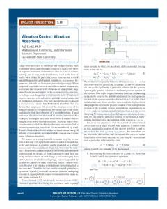
Introduction Shallow arches are common structural members widely used either in civil engineering 共e.g., bridges兲 or in mechanical and aerospace engineering as subelements of more complex structures. More recently, they are being investigated also as components of nanostructures. External resonant excitations may be sources of undesirable flexural vibrations which may be either catastrophic 共due to coupling with torsional modes as, e.g., in the collapse of the Tacoma Narrow Bridge兲 or may significantly reduce the service life due to fatigue. An insidious dynamic instability in these systems is the parametric resonance which can be excited by longitudinal end-displacements or loads above a threshold level 共关1兴兲 and can cause violent and complex vibrations 共关2兴兲. To cope with these large-amplitude vibrations, an open-loop control strategy is developed for a hinged-hinged shallow arch excited by a longitudinal end-displacement which is parametrically resonant with the first antisymmetric mode. The control input is a transverse force at the midspan 共Fig. 1兲. The task of mitigating the effects of resonant disturbances such as parametric excitations has been tackled in a number of different ways ranging from direct disturbance rejection via classical control theory techniques to the use of vibration absorbers attached to the main system as dedicated substructures. For example, a number of works have addressed both theoretically and experimentally the problem of controlling transverse oscillations in distributedparameter systems by parametric-type control actions 共关3,4兴兲 or by coupling autoparametrically the system to an electronic circuit thereby exploiting the saturation phenomenon due to a 2:1 internal 1 To whom all correspondence should be addressed. Contributed by the Applied Mechanics Division of The American Society of Mechanical Engineers for publication in the ASME Journal of Applied Mechanics. Manuscript received by the ASME Applied Mechanics Division, Oct. 18, 2000; final revision, Oct. 25, 2001. Associate Editor: N. C. Perkins. Discussion on the paper should be addressed to the Editor, Prof. Lewis T. Wheeler, Department of Mechanical Engineering, University of Houston, Houston, TX 77204-4792, and will be accepted until four months after final publication of the paper itself in the ASME JOURNAL OF APPLIED MECHANICS.

Journal of Applied Mechanics

resonance mechanism 共关5兴兲. Yabuno et al. 共关6兴兲 showed that a parametric resonance in a cantilever beam can be suppressed by attaching a pendulum absorber to the beam tip. Using a more theoretical framework, Maschke et al. 共关7兴兲 are currently developing a port-controlled Hamiltonian formulation for the dynamics of nonlinear distributed-parameter systems to represent the energy flows through the boundaries of these systems aimed at extending some control schemes proposed for nonlinear finite-dimensional systems 共关8兴兲. When excitations and actuations enter a system at the same point and in the same way, direct cancellation of the disturbance, resulting in no net energy transfer to the system, is possible. In systems such as the one under consideration, wherein the actuation and excitation are noncollocated, direct cancellation of the system disturbance is not possible. Furthermore, the linear modal projection of the control force onto the antisymmetric modes is zero entailing that the system is linearly uncontrollable with the given control input. However, due to the system structural nonlinearities, the nonlinear controller action may be exploited to cancel the external principal parametric resonance. Therefore, the same actuator, optimally collocated to control symmetric modes, may be still employed for controlling antisymmetric modes. One of the objectives of this paper is, in fact, to show how an intelligent exploitation of nonlinear phenomena can greatly expand on the capabilities to control a distributed-parameter system. A direct perturbation expansion of the system dynamics facilitates understanding of the mechanism by which the full nonlinear actuator input may be used to suppress the resonant part of the excitation and further reduce the residual steady-state oscillations. The key mechanism here used is a subharmonic resonance of order one-half arising from the quadratic nonlinearities 共due to initial curvature兲. This work is not the first to examine the effects of the interaction of parametric resonances with subharmonic resonances of order one-half although for single-degree-of-freedom systems only 共关9兴兲. In a previous work by the same authors 共关10兴兲, similar concepts were employed to address noncollocated disturbances

Copyright © 2002 by ASME

MAY 2002, Vol. 69 Õ 325

⳵ 2w ⳵t

2

⫹

⫺

⫺ Fig. 1 Shallow arch geometry with the disturbance and the control input

⳵ 4w ⳵x

4

⳵ 2w ⳵x2

冕

dx

⫽⫺ ⑀ ␯ 2 c

2

0

d␺ 1 d 2␺ dx⫺ ⳵ x dx 2 dx 2

冕冉 冊 1

0

⳵w ⳵x

Equations of Motion and Problem Formulation Nonlinear vibrations of shallow elastic arches around the initial configuration ␺ˆ are governed, in dimensional form, by the following integral-partial-differential equation 共关12兴兲:

m

⳵ 2 wˆ ⳵ 4 wˆ EA d 2 ␺ˆ ⫹EI ⫺ l dxˆ 2 ⳵ ˆt 2 ⳵ xˆ 4 EA ⳵ 2 wˆ ⫺ l ⳵ xˆ 2 ⫺

EA ⳵ 2 wˆ 2l ⳵ xˆ 2

冕 冕冉

冕

⳵ 2 wˆ d ␺ˆ EA uˆ 共 l, ˆt 兲 2 dxˆ ⫺ l ˆ dxˆ ⳵ xˆ 0 ⳵x

d ␺ˆ EA d 2 ␺ˆ dxˆ ⫺ 2l dxˆ 2 ˆ dxˆ 0 ⳵x l

0

⳵ wˆ ⳵ xˆ

冊

冕冉 l

0

⳵ wˆ ⳵ xˆ

冊

2

dxˆ

2

dxˆ

冉 冊

l EA ⳵ wˆ d 2 ␺ˆ ˆ c 共 ˆt 兲 ␦ xˆ ⫺ ⫹ uˆ 共 l, ˆt 兲 2 ⫹U 2 l ⳵ ˆt dxˆ

1

0

⳵w ⳵x

2

dx

2

dx

冉 冊

冉

⳵ 2w ⳵x2

⫹

d 2␺ dx 2

冊

(2)

ˆ c l 4 /(rEI), and ⑀ ␯ 1 u(1,t) where ⑀ ␯ 2 c⫽cˆ l 2 / 冑mEI, ⑀ ␯ 3 U c ⫽U 2 ˆ ˆ ⫽u (l, t )l/r , with ⑀ denoting a small nondimensional number used as a bookkeeping device. For hinged-hinged arches, the boundary conditions are w⫽0 and

⳵ 2w ⳵x2

⫽0 at x⫽0 and x⫽1.

(3)

The linear unforced undamped problem is obtained from Eq. 共2兲 by dropping the damping term, the disturbance, the control force, and the nonlinear terms; that is,

⳵ 2w ⳵t

2

⫹Lw⫽

⳵ 2w ⳵t

2

⫹

⳵ 4w ⳵x

4

⫺

d 2␺ dx

2

冕

d␺ dx⫽0 ⳵ x dx

1⳵ w

0

(4)

with boundary conditions 共3兲. In Eq. 共4兲, L denotes the linear stiffness operator. Because the linear unforced undamped problem is self-adjoint, the eigenfunctions ␾ m (x) are mutually orthogonal and they are normalized as follows: 兰 10 ␾ m ␾ n dx⫽ 具 ␾ m ␾ n 典 ⫽ ␦ mn , 具 ␾ m L␾ n 典 ⫽ ␻ 2n ␦ mn where ␦ mn is the Kronecker delta. For a simplysupported shallow arch with initial shape ␺ (x)⫽b sin ␲x, the eigenmodes are readily obtained in the form of the trigonometric series

␾ n 共 x 兲 ⫽ 冑2 sin n ␲ x, n⫽1,2, . . .

(5)

and the associated natural frequencies are given by ␻ 1 ⫽ ␲ 2 冑1⫹b 2 /2 and ␻ n ⫽n 2 ␲ 2 , n⫽2,3, . . . . A few bimodal twoto-one and one-to-one internal resonances may be possible in hinged-hinged shallow arches. In the next section, we develop an open-loop control strategy to reduce the nonlinear resonant vibrations arising from the boundary-excited principal parametric resonance of the second mode when this mode is away from the mentioned internal resonances.

l⳵ w ˆ

l⳵ w ˆ

冕冉 冊

⳵w 1 ⫹ ⑀ ␯ 3 U c 共 t 兲 ␦ x⫺ ⳵t 2

⫹ ⑀ ␯ 1 u 共 1,t 兲 via nonlinear actuator action in a pendulum-type crane architecture. It is worth pointing out that the use of a perturbation technique, namely the method of multiple scales, is here aimed at designing the type of control inputs rather than simply at obtaining closed-form approximate responses of the system to external disturbances. The control strategy is referred to as ‘‘open loop’’ because neither the system states nor a measured output are employed in direct feedback. Nevertheless, the approach tacitly assumes direct availability of the disturbance levels and relative phases. In practice, these values might be directly measured or estimated through use of an augmented state observer although this may introduce significant complexity. Also, determination of the resonantexcitation character could be extracted from base-excitation measurements by means of phase-locked-loop electronics 共关11兴兲. However, the control methodology is shown to be robust with respect to limited phase and frequency variations.

d␺ dx ⳵ x dx

1⳵ w

1⳵ w

0

1 ⳵ 2w 2 ⳵x2

冕

d 2␺

⫺

(1)

Open-Loop Control Of The Principal Parametric Resonance Of The Second Mode

where m is the mass per unit length; l is the span of the arch; A and I denote the area and moment of inertia of the cross section, respectively; cˆ is the coefficient of linear viscous damping; E is ˆ c ( ˆt ) represent the prescribed endYoung’s modulus; uˆ (l, ˆt ) and U displacement 共external boundary disturbance兲 and the control force at the midspan, respectively; and ␦ denotes the Dirac delta ˆ ). Using the function 共see Fig. 1 for the definitions of ␺ˆ , xˆ , and w following nondimensional variables and parameters: x⫽xˆ /l, ␺ ˆ /r, t⫽ ˆt 冑EI/ml 4 (r is the radius of gyration of the ⫽ ␺ˆ /r, w⫽w cross section兲, Eq. 共1兲 is transformed into its simplest nondimensional form as

In this section, we construct the response of the system to a principal parametric resonance of the second mode when no internal resonances engage this mode with any other mode and the system is subjected to a control force introduced to suppress the principal parametric resonance and further minimize the overall steady-state vibrations. The boundary disturbance is sinusoidal; namely, u(1,t)⫽u B cos ⍀t with ⍀⬇2 ␻ 2 . The ordering of the excitation and damping demands that ␯ 1 ⫽ ␯ 3 ⫽1 and ␯ 2 ⫽2. This ordering promotes the excitation to first order to activate the principal parametric resonance. Further, the control input is introduced also at first order so as to balance and possibly inhibit the external principal parametric resonance. On the other hand, the damping force is demoted to third order where

⫽⫺cˆ

326 Õ Vol. 69, MAY 2002

Transactions of the ASME

there appear the secondary-resonant terms produced by the control force and the resonant effects of the structural nonlinearities yielding the frequency correction. We assume the control signal as a pure tone; that is, U c (t) ⫽U c exp(i(⍀ct⫹␺c))⫹cc where cc denotes the complex conjugate of the preceding term. The objective is to design a control term at first order that is capable of producing resonant terms at second order counteracting the effects of the principal parametric resonance which are proportional to ¯A exp(i␻2t). Here, A indicates the complex-valued amplitude of the arch response at the natural frequency of the second mode ( ␻ 2 ) and the overbar denotes its complex conjugate. Hence, to create nonlinear controller terms at second-order proportional to ¯A exp(i␻2t), the control frequency needs to satisfy the relation ⫾⍀ c ⫾ ␻ 2 ⫽ ␻ 2 . Consequently, we choose ⍀ c ⬇2 ␻ 2 . In addition, it is required that the resulting nonlinear controller action have nonzero projection onto the mode to be controlled 共i.e., the first antisymmetric mode兲. The designed control input is thus expected to produce resonant terms via a one-half subharmonic resonance. The method of multiple scales is employed to determine a third–order uniform expansion of the solutions of 共2兲 and 共3兲. As mentioned, the resonant dynamics arising from the disturbance and control input will appear at second order. However, to capture the nonlinear frequency correction, we seek a third-order expansion. Consequently, one needs to use the method of reconstitution 共关13兴兲. To obtain consistent reconstituted modulation equations, the equations of motion need to be cast as a system of first-order equations in time 共i.e., state-space formulation兲, first, and, then, they can be treated with the method of multiple scales. Therefore, we first rewrite Eq. 共2兲 as a system of two first-order equations in ˙ ⫽ v and putting v˙ instead of w ¨ in time by adding the equation w the equation of motion. Moreover, we directly attack the equations of motion and boundary conditions instead of treating finitedegree-of-freedom discretized versions. In fact, it has been extensively shown that treatment of a discretized set of distributedparameter systems with quadratic and cubic nonlinearities may lead to erroneous quantitative and, in some cases, qualitative results 共关14,15兴兲. Thus, we overcome the problem of order reduction and the associated problems as spillover effects which are critical when designing control laws for such systems. We seek a third-order uniform expansion in the form

Order ⑀ 2 : D 0 w 2 ⫺ v 2 ⫽⫺D 1 w 1 D 0 v 2 ⫹Lw 2 ⫽⫺D 1 v 1 ⫹

兺

k⫽1

兺

k⫽1

D 0 w 1 ⫺ v 1 ⫽0

冉 冊

Journal of Applied Mechanics

0

D 0 v 3 ⫹Lw 3 ⫽⫺D 2 v 1 ⫺D 1 v 2 ⫹ ⫹

⫹

⫹

⳵ 2w 2 ⳵x

2

冕

0

1 ⳵ 2w 1 2 ⳵x2

dx⫹

1 ⳵ 2w 1 共 u B e i⍀T 0 ⫹cc 兲 2 ⳵x2

⳵ 2w 1 ⳵x

2

冕

2 d␺ dx ⳵ x dx

1⳵ w

0

1

冕冉 冊 ⳵w1 ⳵x

1

0

(11)

冕

1⳵ w

0

1

⳵x

⳵w2 dx ⳵x

2

dx⫺2 ␮ v 1

1 ⳵ 2w 2 共 u B e i⍀T 0 ⫹cc 兲 2 ⳵x2

(12)

The boundary conditions at all orders are given by 共3兲. Because the second mode is directly excited by the principal parametric resonance of the disturbance and indirectly by the subharmonic resonance of the control input; moreover, because there are no internal resonances involving this mode, we assume the solution at order ⑀ as w 1 ⫽A 共 T 1 ,T 2 兲 e i ␻ 2 T 0 ␾ 2 共 x 兲 ⫹Uc 共 x 兲 e i(⍀T 0 ⫹ ␺ c ) ⫹B共 x 兲 e i⍀T 0 ⫹cc

(13)

where the functions Uc (x) and B(x) are solutions of the following boundary value problems:

冉 冊

1 1 LUc ⫺4 ␻ 22 Uc ⫽ U c ␦ x⫺ 2 2

(14)

1 d 2␺ LB⫺4 ␻ 22 B⫽ u B 2 . 2 dx

(15)

The function Uc can be expressed as an infinite series of the eigenfunctions in the form ⬁

␾ 2k⫹1 共 1/2兲 1 Uc 共 x 兲 ⫽ U c ␾ 2k⫹1 共 x 兲 2 2 k⫽0 ␻ 2k⫹1 ⫺4 ␻ 22 ⫽

Uc

␲

4

冋

兺

⬁

2

兺

sin ␲ x⫹ k⫽1 b ⫺126 2

册

sin共共 2k⫹1 兲共 ␲ /2兲兲 共 2k⫹1 兲 4 ⫺64

⫻sin共 2k⫹1 兲 ␲ x .

(16)

On the other hand, the function B can be readily obtained as B共 x 兲 ⫽⫺

(8)

2

d␺ d 2␺ dx⫹ 2 ⳵ x dx dx

1⳵ w

(7)

1 1 D 0 v 1 ⫹Lw 1 ⫽ U c e i(⍀T 0 ⫹ ␺ c ) ␦ x⫺ 2 2 1 d 2␺ ⫹ u e i⍀T 0 ⫹cc 2 dx 2 B

⳵w1 ⳵x

冕冉 冊

D 0 w 3 ⫺ v 3 ⫽⫺D 2 w 1 ⫺D 1 w 2

(6)

where T k ⫽ ⑀ k t are the time scales. Then, the first derivative with respect to time is defined as ⳵ / ⳵ t⫽D 0 ⫹ ⑀ D 1 ⫹ ⑀ 2 D 2 ⫹••• where D n ⫽ ⳵ / ⳵ T n . To express the nearness of the principal parametric resonance, we introduce the detuning parameter ␴ such that ⍀ ⫽2 ␻ 2 ⫹ ⑀ ␴ . We assume at this stage that the excitation and control signals are phase-locked and one-to-one; that is, ⍀ c ⫽⍀ 共this assumption will be later relaxed兲. Substituting 共6兲 into the system of first-order 共in time兲 equations of motion and boundary conditions 共3兲, using the independence of the time scales, and equating coefficients of like powers of ⑀ yields Order ⑀:

1

0

1

Order ⑀ :

⑀ k w k 共 x,T 0 ,T 1 ,T 2 兲 ⫹••• ⑀ k v k 共 x,T 0 ,T 1 ,T 2 兲 ⫹•••

⳵x

d␺ dx ⳵ x dx

1⳵ w

(10)

3

v共 x,t 兲 ⫽

冕

2

3

3

w 共 x,t 兲 ⫽

1 d 2␺ 2 dx 2

⫹

⳵ 2w 1

(9)

uB

␲ 共 b ⫺126兲 2

2

b sin ␲ x.

(17)

Substituting 共13兲 and v 1 ⫽D 0 w 1 into the second-order problem, Eqs. 共9兲 and 共10兲, we obtain D 0 w 2 ⫺ v 2 ⫽⫺ 共 D 1 A 兲 e i ␻ 2 T 0 ␾ 2 共 x 兲 ⫹cc

(18)

MAY 2002, Vol. 69 Õ 327

冉

冊

1 ¯ e i( ␻ 2 T 0 ⫹ ␴ T 1 ) ␾ ⬙2 具 B⬘ ␺ ⬘ 典 ⫹ u B ⫹e i ␺ c 具 U⬘c ␺ ⬘ 典 D 0 v 2 ⫹Lw 2 ⫽⫺i ␻ 2 共 D 1 A 兲 e i ␻ 2 T 0 ␾ 2 共 x 兲 ⫹A 2 1 1 ⫹Ae i(3 ␻ 2 T 0 ⫹ ␴ T 1 ) ␾ ⬙2 具 B⬘ ␺ ⬘ 典 ⫹ u B ⫹e i ␺ c 具 U⬘c ␺ ⬘ 典 ⫹e i(4 ␻ 2 T 0 ⫹2 ␴ T 1 ⫹2 ␺ c ) ␺ ⬙ 具 U⬘c U⬘c 典 ⫹U ⬙c 具 U⬘c ␺ ⬘ 典 2 2 1 ⫹e i(4 ␻ 2 T 0 ⫹2 ␴ T 1 ⫹ ␺ c ) U ⬙c 具 B⬘ ␺ ⬘ 典 ⫹B⬙ 具 U⬘c ␺ ⬘ 典 ⫹ ␺ ⬙ 具 U⬘c B⬘ 典 ⫹ u B U ⬙c 2 1 1 ⫹e i(4 ␻ 2 T 0 ⫹2 ␴ T 1 ) ␺ ⬙ 具 B⬘ B⬘ 典 ⫹B⬙ 具 B⬘ ␺ ⬘ 典 ⫹ u B B⬙ 2 2 1 1 ¯ ␺ ⬙ 具 ␾ ⬘2 ␾ ⬘2 典 ⫹e i ␺ c 共 U ⬙c 具 B⬘ ␺ ⬘ 典 ⫹B⬙ 具 U ⬘c ␺ ⬘ 典 ⫹ ␺ ⬙ 具 U ⬘c B⬘ 典 兲 ⫹U ⬙c 具 U ⬘c ␺ ⬘ 典 ⫹ A 2 e 2i ␻ 2 T 0 ␺ ⬙ 具 ␾ ⬘2 ␾ ⬘2 典 ⫹ AA 2 2 1 1 1 ⫹ ␺ ⬙ 具 U ⬘c U c⬘ 典 ⫹B⬙ 具 B⬘ ␺ ⬘ 典 ⫹ ␺ ⬙ 具 B⬘ B⬘ 典 ⫹ u B B⬙ ⫹cc 2 2 2

冉 冉

冉

¯ e i ␴ T 1 共 K 1 ⫹e i ␺ c K 2 兲 2i ␻ 2 D 1 A⫽A

(20)

where the external parametric excitation coefficient and the subharmonic control gain are given, respectively, by

冊

1 252␲ K 1 ⫽ 具 ␾ 2⬙ ␾ 2 典 具 B⬘ ␺ ⬘ 典 ⫹ u B ⫽ 2 uB 2 b ⫺126 2

(21)

and

冉

冊

冊

where the prime indicates differentiation with respect to x. Because the associated homogeneous problem admits nontrivial solutions, the resulting inhomogeneous problem, Eqs. 共18兲, 共19兲, and 共3兲, possesses solutions only if solvability conditions are satisfied. The solvability conditions of Eqs. 共18兲, 共19兲, and 共3兲 demand that the right-hand side of Eqs. 共18兲 and 共19兲 be orthogonal to every solution of the associated adjoint homogeneous problem. The transposes of the solutions of the adjoint homogeneous problem are (i ␻ k ,1) ␾ k (x)exp(⫺i␻kT0). Hence, imposing that the righthand side of Eqs. 共18兲 and 共19兲 be orthogonal to these adjoints, we obtain the following solvability condition:

冉

冊

冊

2i ␻ 2 共 D 2 A⫹ ␮ A 兲 ⫽ ␣ A 2 ¯A ⫹ ␴ s A

(19)

(25)

where the effective nonlinearity coefficient is given by

冋

3 ␣ ⫽ 具 ␾ 2 ␾ 2⬙ 典 2 具 ␺ ⬘ ␹ 4⬘ 典 ⫹ 具 ␺ ⬘ ␹ 3⬘ 典 ⫹ 具 ␾ 2⬘ ␾ 2⬘ 典 2

冋冉

⫽8 ␲ 4 b 2

2 b ⫹2 2

1

⫹

b ⫺126 2

冊 册

册

⫺3 .

(26)

On the other hand, the coefficient of the linear frequency shift is given by

␴ s⫽

16U 2c

冋

b2

共 b 2 ⫹2 兲 ␲ 4 共 b 2 ⫺126兲

⫹

⫺ 2

␲ 2 (⬁) S 2 1

500␲ 2 b 2 u B2 ⫺16b 共 b 2 ⫺1 兲 U c u B

␲ 共 b ⫹2 兲共 b ⫺126兲 2

2

2

2

册 ⫹

共 63␲ 2 u B ⫺U c b 兲 2

4 ␲ 4 共 b 2 ⫺126兲 2 (27)

K 2 ⫽ 具 ␾ ⬙2 ␾ 2 典具 U⬘c ␺ ⬘ 典 ⫽⫺

4b b 2 ⫺126

Uc .

(22)

Substituting 共20兲 into 共18兲 and 共19兲, we seek the solutions of the resulting equations along with 共3兲 in the form w 2 ⫽ 关 ␹ 1 共 x 兲 ⫹e i ␺ c ␹ 2 共 x 兲兴 ¯A e i( ␻ 2 T 0 ⫹ ␴ T 1 ) ⫹ ␹ 3 共 x 兲 A 2 e 2i ␻ 2 T 0 ¯ ⫹ 关 ␹ 5 共 x 兲 ⫹e i ␺ c ␹ 6 共 x 兲兴 Ae i(3 ␻ 2 T 0 ⫹ ␴ T 1 ) ⫹ ␹ 4 共 x 兲 AA ⫹ 关 ␹ 7 共 x 兲 ⫹e ⫹e

i␺c

i␺c

␹ 8 共 x 兲 ⫹e

2i ␺ c

␹ 9 共 x 兲兴 e

i(4 ␻ 2 T 0 ⫹2 ␴ T 1 )

2i ␻ 2 共 A˙ ⫹ ␮ A 兲 ⫽ 共 K 1 ⫹e i ␺ c K 2 兲 e i ␴ t ¯A ⫹ ␴ s A⫹ ␣ A 2 ¯A . ⫹ ␹ 10共 x 兲

␹ 11共 x 兲 ⫹cc

(23)

A e i( ␻ 2 T 0 ⫹ ␴ T 1 ) ⫹ ␩ 3 共 x 兲 A 2 e 2i ␻ 2 T 0 v 2 ⫽ 关 ␩ 1 共 x 兲 ⫹e i ␺ c ␩ 2 共 x 兲兴 ¯ ¯ ⫹ 关 ␩ 5 共 x 兲 ⫹e ⫹ ␩ 4 共 x 兲 AA

i␺c

␩ 6 共 x 兲兴 Ae

i(3 ␻ 2 T 0 ⫹ ␴ T 1 )

⫹ 关 ␩ 7 共 x 兲 ⫹e i ␺ c ␩ 8 共 x 兲 ⫹e 2i ␺ c ␩ 9 共 x 兲兴 e i(4 ␻ 2 T 0 ⫹2 ␴ T 1 ) ⫹ ␩ 10共 x 兲 ⫹e i ␺ c ␩ 11共 x 兲 ⫹cc.

(24)

The second-order displacement and velocity fields depend on the shape functions ␹ j and ␩ j . The functions ␹ j are solutions of a number of boundary value problems, Eqs. 共40兲–共49兲 with boundary conditions 共50兲, reported in the Appendix. The functions governing the system response at first and second-order are shown in Fig. 2 for the values b⫽16.5, u B ⫽1, and U c ⫽28.936. Using the solutions at second order, Eqs. 共23兲 and 共24兲, and substituting them into the third-order problem, Eqs. 共11兲 and 共12兲, we impose the solvability condition governing at this order the dependence of A on the scale T 2 ; that is, 328 Õ Vol. 69, MAY 2002

where use of the phase condition ␺ c ⫽2n ␲ was made 共this condition will be discussed in the next section兲. Employing the method of reconstitution by substituting 共20兲 and 共25兲 into A˙ ⫽ ⑀ D 1 A⫹ ⑀ 2 D 2 A⫹ . . . , and setting ⑀ ⫽1, we obtain the normal form governing the modulation of the amplitude and phase as (28)

The deflection of the arch, to second order, is given by the sum of 共13兲 and 共23兲 with the complex-valued amplitude A being governed by the reconstituted modulation Eq. 共28兲. Control Input Design. Our objective is the reduction of the overall parametrically excited vibrations. Therefore, to optimize the nonlinear control action, we choose the following cost functional: max J⫽

0⭐t⭐T c

再冕

1

0

w 共 x,t;a m 兲 2 dx

冎

(29)

where T c is the period of oscillation and a m is the maximum stable value of the real part of the complex-valued amplitude A at the disturbance frequency detuning ␴ . This cost is calculated based on steady-state rather than transient behavior. Hence, it reflects the cost predicted over long periods of operation where transient effects are negligible. The constraint for the optimization problem is given by the reconstituted modulation Eq. 共28兲. The domain where minimization of J is sought is spanned by U c and ␺ c . It is clear that if we seek conditions for minimizing a m , then Transactions of the ASME

Fig. 2 First and second-order shape functions: „a… Uc ; „b… B; „c… ␹ 1 and ␹ 2 ; „d… ␹ 3 and ␹ 4 ; „e… ␹ 5 and ␹ 6 ; „f … ␹ 7 ; „g… ␹ 8 ; „h… ␹ 9 ; „i … ␹ 10 ; and „ j… ␹ 11 when b Ä16.5, u B Ä1.0, and U c Ä28.936

we can more efficiently minimize J within the design parameter subset where the minimum of a m is attained. The form of the effective parametric excitation coefficient 共sum of the external parametric and subharmonic control coefficients兲 suggests that we have the ability to affect this coefficient through the control gain and phase. Then, the objective is to lower this coefficient below the activation threshold of the parametric resonance. In this way, we prevent the principal parametric resonance from being activated and the only stable solution becomes the trivial solution. It is clear that the magnitude of the overall effective parametric resonance coefficient—K 1 ⫹K 2 exp(i␺c)—is minimum with respect to changes in the control phase when K 2 exp(i␺c) lies in a complex-vector direction opposite to K 1 . Inspecting Eqs. 共21兲 and 共22兲, we note that K 1 and K 2 have always opposite sign; hence, the control phase condition is easily obtained as ␺ c ⫽2n ␲ , n ⫽0,1, . . . . Using this condition, we can transform the complexvalued modulation Eq. 共28兲 into the real-valued modulation equations for the amplitude and phase. To this end, we assume the following polar transformation A⫽1/2a exp(i␤)exp(⫺i␴s/2t) and obtain the phase ␥ ⫽( ␴ ⫹ ␴ s )t⫺2 ␤ in order to render the modulation equations autonomous. Substituting the polar transformation into 共28兲 and using the control phase condition 共i.e., ␺ c ⫽2n ␲ ) yields 1 Ke a sin ␥ 2 ␻2

(30)

␴s ␣ 3 Ke ⫹ a ⫹ a cos ␥ , ␻2 4␻2 ␻2

(31)

a˙ ⫽⫺ ␮ a⫹

冉

a ␥˙ ⫽a ␴ ⫹

冊

where K e ⫽K 1 ⫹K 2 . The frequency-response equation for the steady-state amplitude is given by

␴ ⫽⫺

冉

冊冑

␴s ␣ 2 ⫹ a ⫾ ␻2 4␻2

Journal of Applied Mechanics

K 2e

␻ 22

⫺4 ␮ 2

(32)

whereas the phase is given by tan␥ ⫽⫿ ␮ (K 2e /4␻ 22 ⫺ ␮ 2 ) ⫺(1/2) . We gain more insight into the effects of the control scheme by preliminarily investigating the system uncontrolled dynamics excited by the principal parametric resonance. In this case, the frequency-response equation can be obtained from 共32兲 by putting U c ⫽0 into ␴ s and K e 共hence, K e ⫽K 1 ). The amplitudes of the nontrivial uncontrolled responses are given by

冋 冉

␣ ␴ s,uc a⫽2 ⫺␴⫺ ⫾ ␻2 ␻2

冑

K 21

␻ 22

⫺4 ␮

2

冊册

1/2

.

(33)

Seeking conditions for the existence of real solutions for a, we conclude that there are three regions in the plane of disturbance amplitude and detuning as shown in Fig. 3 共where b⫽16.5 and ␮ ⫽0.05). Namely, 共i兲 in region I (u B ⬍u B,cr ᭙ ␴ or ␴ ⬎ ⫺ ␴ s,uc / ␻ 2 ⫹(K 21 / ␻ 22 ⫺4 ␮ 2 ) 1/2), there are no solutions; 共ii兲 in region II (⫺ ␴ s,uc / ␻ 2 ⫺(K 21 / ␻ 22 ⫺4 ␮ 2 ) 1/2⬍ ␴ ⬍⫺ ␴ s,uc / ␻ 2 2 2 2 1/2 ⫹(K 1 / ␻ 2 ⫺4 ␮ ) ), there is only one real solution; 共iii兲 in region III ( ␴ ⬍⫺ ␴ s,uc / ␻ 2 ⫺(K 21 / ␻ 22 ⫺4 ␮ 2 ) 1/2), there are two real solutions. We note that subregion I⬘ 共i.e., u B ⬍u B,cr ), embedded in region I, is such that the nonactivation of the parametric resonance therein is independent of the frequency detuning. The activation threshold is obtained from 共33兲 imposing vanishing of the argument of the inner square root which yields u B,cr ⫽2 ␮ 兩 b 2 ⫺126兩 /63. Computation of the effective nonlinearity coefficient, when b ⫽16.5, leads to ␣ ⫽660.008. The linear frequency shift is ␴ s,uc ⫽6.9599⫻10⫺2 . In Fig. 4, we show the frequency-response curve of the uncontrolled case when u B ⫽1 and ␮ ⫽0.05. Clearly, for the considered sag level, the second mode of the arch is of the softening type. Point S 1 (S 2 ) corresponds to a supercritical 共subcritical兲 pitchfork bifurcation. In the presence of control input, the activation threshold for the parametric resonance is obtained from 共32兲 letting K 2e ⫽4 ␮ 2 ␻ 22 . MAY 2002, Vol. 69 Õ 329

Fig. 3 Regions of activationÕnonactivation of the principal parametric resonance in the plane of the disturbance frequency detuning and gain when b Ä16.5 and ␮ Ä0.05

Substituting the expressions 共21兲 and 共22兲 for K 1 and K 2 into K e for fixed disturbance level and damping, we determine the range of control gain where the parametric resonance is not activated as (2) U (1) where U (1,2) ⫽63␲ 2 /b(u B ⫿u B,cr ). Within this c ⬍U c ⬍U c c range 共lightly shaded region in Fig. 5兲, there is a locus of control gains where the effective parametric coefficient becomes zero; 2 that is, U (3) c ⫽63␲ u B /b. It is worth emphasizing that requiring the control gain to be within the cancellation region in Fig. 5 entails enforcing the system to be in subregion I⬘ 共Fig. 3兲 where the parametric resonance is annihilated for any frequency detuning. It is interesting to investigate the sensitivity of the developed control strategy to variations in the relative phase and frequency detuning. We first investigate the effect of the phase variations with perfect frequency tuning 共i.e., ⍀⫽⍀ c ). To this end, the analysis is simplified by neglecting third-order contributions which are not expected to influence significantly the resonance activation threshold. The region of resonance cancellation is obtained as K 21 ⫹K 22 ⫹2K 1 K 2 cos␺ c ⭐4 ␮ 2 ␻ 22 .

(34)

Substituting the expressions for K 1 and K 2 into 共34兲, we obtain the cancellation regions in the plane of disturbance and control gains for different phase angles ␺ c . Evidently, on account of 共34兲, the regions are independent of the sign of ␺ c . Further, it can be shown that the cancellation regions are physically meaningful when ␺ c 苸(⫺ ␲ /2,␲ /2). Figure 5 shows clearly that ␺ c ⫽2n ␲ is the optimal phase angle because the associated region is nonterminating indicating that, in principle, cancellation is achievable for any disturbance level. A variation of ␺ c by 6 deg renders the region terminating thereby entailing that past a disturbance threshold, cancellation cannot be achieved. However, this occurs for rather high values of disturbances. On the other hand, for low-tomedium excitation amplitudes, small changes in phase angle do not practically vary the cancellation region. Nevertheless, Fig. 5 also shows that significant increases in phase angle variations, as expected, degrade the control performance until it becomes ineffective when ␺ c ⫽ ␲ /2.

Results And Discussion Within the outlined regions of resonance cancellation 共Fig. 5兲, the optimal gains are determined via the presented optimization scheme. Therefore, for the given nondimensional sag b⫽16.5, damping coefficient ␮ ⫽0.05, and disturbance level u B ⫽1, we computed the cost when U c varies in the range U (1) c ⫽28.936 to U (2) c ⫽46.432 where the parametric resonance is cancelled and determine, accordingly, the optimal control gain as the value where the cost is minimum. Clearly, in this case, the only stable solution for the amplitude is the trivial solution. Accordingly, the solution for the displacement field at steady state can be expressed as w 共 x,t 兲 ⫽2 cos ⍀t 关 B共 x 兲 ⫹Uc 共 x 兲兴 ⫹2 兵 cos共 2⍀t 兲关 ␹ 7 共 x 兲 ⫹ ␹ 8 共 x 兲 ⫹ ␹ 9 共 x 兲兴 ⫹ ␹ 10共 x 兲 ⫹ ␹ 11共 x 兲 其 .

Fig. 4 Frequency-response curve of the uncontrolled arch when b Ä16.5, ␮ Ä0.05, and u B Ä1. Solid „dashed… line indicates stable „unstable… solutions.

330 Õ Vol. 69, MAY 2002

(35)

Thus, using 共35兲, we computed w(x,t) when U c is equal to (2) (3) U (1) c , U c , and U c . Here, we note that the convergence of the first and second-order shape functions expressed as infinite series is very fast. In fact, numerical tests conducted with MATHEMATICA, showed that, for the given sag level, three/four terms are sufficient for convergence. Using five terms, we obTransactions of the ASME

Fig. 5 Regions „shaded… of nonactivation of the principal parametric resonance in the plane of the disturbance and control gains for different control phase angles when b Ä16.5 and ␮ Ä0.05

⫺5 tained S (5) and 共i兲 K 1 ⫽17.006, K 2 ⫽⫺13.058, 1 ⫽1.6341⫻10 ⫺3 and ␴ s ⫽⫺7.6441⫻10 when U c ⫽28.936; 共ii兲 K 1 ⫽⫺K 2 ⫽17.006, and ␴ s ⫽⫺1.926⫻10⫺2 when U c ⫽63␲ 2 u B /b ⫽37.684; 共iii兲 K 1 ⫽17.006, K 2 ⫽⫺20.954, and ␴ s ⫽⫺2.543 ⫻10⫺2 when U c ⫽46.432. Computation of the cost according to Eq. 共29兲 shows that it is minimum when U c ⫽U (1) c ⫽28.936. Hence, we assume this control gain as the optimal control gain. It is interesting to compare the optimally controlled case with the uncontrolled case when the frequency detuning is ␴ ⫽⫺10 and u B ⫽1, b⫽16.5, and ␮ ⫽0.05. First, we compare the steadystate responses. Then, we compare the transient responses in the presence of initial conditions within the basin of attraction of the uncontrolled parametrically resonant response. The steady-state deflection for the controlled case is given by 共35兲. On the other hand, the steady-state uncontrolled displacement field, to second order, is expressed as

冋

w 共 x,t 兲 ⫽a cos

册

1 共 ⍀t⫺ ␥ 兲 ␾ 2 共 x 兲 ⫹2 cos ⍀tB共 x 兲 2

冋

⫹a cos

册

1 共 ⍀t⫹ ␥ 兲 ␹ 1 共 x 兲 ⫹2 cos 共 2⍀t 兲 ␹ 7 共 x 兲 2

1 ⫹ a 2 关 cos共 ⍀t⫺ ␥ 兲 ␹ 3 共 x 兲 ⫹ ␹ 4 共 x 兲兴 2

冋

⫹a ␹ 5 共 x 兲 cos

册

1 共 3⍀t⫺ ␥ 兲 ⫹2 ␹ 10共 x 兲 2

(36)

where ␹ 10 is given by 共61兲 inserting U c ⫽0 in it. We computed the stable steady-state response amplitude and phase when ␴ ⫽⫺10 and u B ⫽1 and found a⫽1.579 and ␥ ⫽⫺13.42 deg. The period of oscillation is T⫽0.182 and the cost is J⫽2.890. In Fig. 6, we show the uncontrolled steady-state deflections contrasted with the optimally controlled deflections 共magnified ten times in the scale of the uncontrolled deflections兲 Journal of Applied Mechanics

Fig. 6 Uncontrolled „thin line… and optimally controlled „thick line… dynamic deflections at seven discrete times equally spaced within a period of oscillation when b Ä16.5, ␮ Ä0.05, u B Ä1, ␴ ÄÀ10, and U c Ä28.936

MAY 2002, Vol. 69 Õ 331

Fig. 7 Time histories of the uncontrolled and optimally controlled deflections „ ␺ c Ä0 and U c Ä28.936… at x Ä1Õ4 when u B Ä1, ␴ ÄÀ10, b Ä16.5, ␮ Ä0.05, p „0…Ä1.5, and q „0…ÄÀ0.95

at seven discrete times equally spaced in a period of the uncontrolled oscillations 共twice the period of the controlled oscillations兲. The result is that the overall optimally controlled deflection at steady state is two orders of magnitude smaller than that of the uncontrolled case and the relative decrease of the cost is 97.5%. Finally, to contrast the behavior of the uncontrolled response with the optimally controlled response in the transient regime, we cast the modulation equations and the displacement field in Cartesian form by using the transformation A⫽1/2/(p ⫺iq)exp(i␴/2t). Using this transformation, the modulation equations become

冉 冉

冊 冊

p˙ ⫽⫺ ␮ p⫹

1 Ke 1 ␣ 2 ␴s ⫺␴⫺ q⫺ 共 p ⫹q 2 兲 q 2 ␻2 ␻2 8 ␻2

(37)

q˙ ⫽⫺ ␮ q⫹

1 Ke 1 ␣ 2 ␴s ⫹␴⫹ p⫹ 共 p ⫹q 2 兲 p. 2 ␻2 ␻2 8 ␻2

(38)

The displacement field, to second order, is also expressed in terms of Cartesian components as

冉

冊

⍀ ⍀ w 共 x,t 兲 ⫽ p cos t⫹q sin t ␾ 2 共 x 兲 ⫹2 cos ⍀t 共 B共 x 兲 ⫹Uc 共 x 兲兲 2 2

冉 冉

冊

⍀ ⍀ ⫹ p cos t⫺q sin t 共 ␹ 1 共 x 兲 ⫹ ␹ 2 共 x 兲兲 2 2

冊

3⍀ 3⍀ t⫹q sin t 共 ␹ 5 共 x 兲 ⫹ ␹ 6 共 x 兲兲 ⫹ p cos 2 2 ⫹2 cos共 2⍀t 兲共 ␹ 7 共 x 兲 ⫹ ␹ 8 共 x 兲 ⫹ ␹ 9 共 x 兲兲

1 ⫹ 关共 p 2 ⫺q 2 兲 cos ⍀t⫹2pq sin ⍀t 兴 ␹ 3 共 x 兲 2 1 ⫹ 共 p 2 ⫹q 2 兲 ␹ 4 共 x 兲 ⫹2 共 ␹ 10共 x 兲 ⫹ ␹ 11共 x 兲兲 . 2

(39)

We integrated Eqs. 共37兲 and 共38兲 using a variable stepsize fifthorder Runge-Kutta scheme when p(0)⫽1.5 and q(0)⫽⫺0.95 for the optimally controlled and uncontrolled cases. Using Eq. 共39兲, we computed the time histories of the deflections at x⫽1/4 in whose neighborhood the maximum vibration amplitude is attained and show the results in Fig. 7. We note that, after the transient dies out, the response in the controlled case is two orders of magnitude smaller than that in the uncontrolled case. Evidently, as expected, the decay rate of the transients in the controlled case is not affected by the control strategy. Last, to show the robustness of the control strategy with respect to variations in frequency detuning, we performed some numeri cal tests. To this end, we introduced the control frequency detuning as ⍀ c ⫽2 ␻ 2 ⫹ ⑀ ␴ c and carried out the perturbation expansion up to second order. We integrated the obtained nonautonomous modulation equations in Cartesian form using the same parameters chosen thus far with different values of frequency detuning defined as ⌬ ␴ ⫽ ␴ ⫺ ␴ c . We found that resonance cancellation is achieved for a wide range of positive and negative frequency detunings 共i.e., excitation frequency lower or greater than the control frequency兲 with differences with respect to the perfectly tuned case in the transient regime only. A small range of positive detunings 共approximately 9.7 to 10兲 was found where cancellation can-

Fig. 8 Time histories of the controlled deflections „second-order solution… at x Ä1Õ4 in the detuned case when „a… ⌬ ␴ Ä ␴ À ␴ c ÄÀ9.55 and „b… ⌬ ␴ Ä8.95 and ␺ c Ä0, U c Ä28.936, ␴ ÄÀ10, b Ä16.5, ␮ Ä0.05, u B Ä1, p „0…Ä1.5, and q „0…ÄÀ0.95

332 Õ Vol. 69, MAY 2002

Transactions of the ASME

not be achieved resulting in unbounded growth of the response in the investigated second-order solution. However, past this range, cancellation is recovered again. Figure 8 shows the response of the system in two detuned cases when 共a兲 ⌬ ␴ ⫽⫺9.55 with a frequency variation of about 13.8% and 共b兲 ⌬ ␴ ⫽8.95 with a frequency variation of about 13%. While in the negatively detuned case, no appreciable differences are noted, in the positively detuned case 共prior the onset of instability at ⌬ ␴ ⬇9.7), the presence of a large-amplitude excursion in the initial phase of the motion and modulation in the response are observed although the response decays with the same rate as in the perfectly tuned case.

1 L␹ 8 ⫺16␻ 22 ␹ 8 ⫽U ⬙c 具 B⬘ ␺ ⬘ 典 ⫹B⬙ 具 U⬘c ␺ ⬘ 典 ⫹ ␺ ⬙ 具 U⬘c B⬘ 典 ⫹ u B U ⬙c 2 (46) 1 L␹ 9 ⫺16␻ 22 ␹ 9 ⫽U ⬙c 具 U⬘c ␺ ⬘ 典 ⫹ ␺ ⬙ 具 U⬘c U⬘c 典 2

(47)

1 1 L␹ 10⫽B⬙ 具 B⬘ ␺ ⬘ 典 ⫹ ␺ ⬙ 具 B⬘ B⬘ 典 ⫹ u B B⬙ ⫹U c⬙ 具 U⬘c ␺ ⬘ 典 2 2 1 ⫹ ␺ ⬙ 具 U⬘c U⬘c 典 2

(48)

L␹ 11⫽B⬙ 具 U⬘c ␺ ⬘ 典 ⫹U ⬙c 具 B⬘ ␺ ⬘ 典 ⫹ ␺ ⬙ 具 U⬘c B⬘ 典

Conclusions In this work we have demonstrated the effectiveness of a nonlinear control strategy to cancel the parametrically forced oscillations of a shallow arch and further minimize the residual nonresonant oscillations. In particular, the control strategy inhibits activation of the principal parametric resonance using a point actuator at the midspan of the arch. The control algorithm is open loop because state parameters are not used for feedback. The difficulty arises because the disturbance input and actuator are not physically collocated and the control action is linearly orthogonal to the excited mode 共first antisymmetric mode兲. The key idea is to rely on part of the nonlinear controller action which is not orthogonal to the mode and further has resonant effects onto it. We show that a perturbation analysis can be used to develop intuition as to the proper form of the control input. In this paper, a one-half subharmonically resonant control law is used for sup pressing the parametric resonance by enforcing the effective parametric resonance coefficient to be below the activation threshold. This condition yields the control input in phase with the disturbance in the optimal case. On the other hand, the optimal gain value that minimizes the resulting steady-state vibrations, according to a chosen cost functional, is also determined. The technique is shown to reduce the overall vibrations by orders of magnitude with respect to the uncontrolled case. The robustness of the proposed control methodology with respect to phase and frequency variations has also been demonstrated. Application of perturbation techniques to problems of this type seems to provide a unified approach that may be applicable to a broad class of weakly nonlinear distributed-parameter systems with either noncollocated inputs or linearly uncontrollable modes.

subject to the boundary conditions

␹ i ⫽0 and ␹ i⬙ ⫽0 at x⫽0 and x⫽1.

␩ j ⫽i ␻ 2 ␹ j ⫺i ␩ 3 ⫽2i ␻ 2 ␹ 3 ,

L␹ j ⫺ ␻ 22 ␹ j ⫽0,

j⫽1,2

1 L␹ 4 ⫽ ␺ ⬙ 具 ␾ ⬘2 ␾ ⬘2 典 2

(42)

L␹ 5 ⫺9 ␻ 22 ␹ 5 ⫽ ␾ 2⬙

冋

1 具 B⬘ ␺ ⬘ 典 ⫹ u B 2

L␹ 6 ⫺9 ␻ 22 ␹ 6 ⫽ ␾ ⬙2 具 U⬘c ␺ ⬘ 典 L␹ 7 ⫺16␻ 22 ␹ 7 ⫽B⬙ 具 B⬘ ␺ ⬘ 典 ⫹ Journal of Applied Mechanics

冋

␹ j⫽

Kj 4 ␻ 22

1 1 ␺ ⬙ 具 B⬘ B⬘ 典 ⫹ u B B⬙ 2 2

(43) (44) (45)

j⫽5,6

(52)

␩ 10⫽ ␩ 11⫽0

(53)

册

Kj ␾ 共 x 兲, 2␻2 2

␩ j ⫽⫺i ␻ 2 ␹ j ,

␾ 2共 x 兲 ,

j⫽1,2. (54)

j⫽1,2.

(55)

Solving the remaining boundary value problems 共41兲–共49兲 with boundary conditions 共50兲, we obtain the following shape functions: 4b

␹ 3 ⫽⫺

sin␲ x, b ⫺126 2

63u B

␾2 ,

32␲ 2 共 b 2 ⫺126兲

␹ 4 ⫽⫺ ␹ 6⫽

4b b ⫹2 2

sin␲ x

bU c 32␲ 4 共 b 2 ⫺126兲

(56)

␾2 , (57)

␹ 7 ⫽⫺

u B2 b 共 b 2 ⫹252兲 2 ␲ 4 共 b 2 ⫺126兲 2 共 b 2 ⫺510兲

U cu B

␲ 6 共 b 2 ⫺126兲 ⬁

兺

k⫽1

冋

再

␹ 9 ⫽⫺ ⫺

2bU 2c

共 b 2 ⫺126兲共 b 2 ⫺510兲

关共 2k⫹1 兲 4 ⫺256兴关共 2k⫹1 兲 4 ⫺64兴

冋

冎

2

bU 2c

␲ 8 共 b 2 ⫺126兲

⫻sin共 2k⫹1 兲 ␲ x

⬁

兺

k⫽1

2

再

册 (59)

2 4

(58)

sin ␲ x

s 2k⫹1 共 2k⫹1 兲 2

␲ 共 b ⫺510兲 ␲ 共 b ⫺126兲 4

sin ␲ x

4 共 b 2 ⫹63兲

⫻sin共 2k⫹1 兲 ␲ x

册

(51)

To remove the indeterminacy associated with the arbitrary constants d j , we impose that the functions ␹ 1 and ␩ 1 and ␹ 2 and ␩ 2 are orthogonal to the adjoint (i ␻ 2 ,1) ␾ 2 (x). The result is

⫹63 (41)

j⫽7,8,9,

␩ j ⫽i ␻ 2 d j ⫺

␹ j ⫽d j ␾ 2 共 x 兲 ,

(40)

1 L␹ 3 ⫺4 ␻ 22 ␹ 3 ⫽ ␺ ⬙ 具 ␾ 2⬘ ␾ 2⬘ 典 2

j⫽1,2

␩ j ⫽3i ␻ 2 ␹ j ,

␩ j ⫽4i ␻ 2 ␹ j ,

␹ 8⫽

Boundary Value Problems And Solutions.

Kj ␾ , 2␻2 2

Solving 共40兲 and 共50兲 and using 共51兲, we obtain

This work was partially supported by a M.U.R.S.T. COFIN992000 grant. Interesting comments by one of the reviewers are gratefully acknowledged.

Appendix

(50)

The functions ␩ j , in turn, are given by

␹ 5 ⫽⫺

Acknowledgments

(49)

2

⫹

册

␲ 2 (⬁) S sin ␲ x 2 1

s 2k⫹1 共 2k⫹1 兲 2 关共 2k⫹1 兲 4 ⫺256兴关共 2k⫹1 兲 4 ⫺64兴

冎

(60) MAY 2002, Vol. 69 Õ 333

␹ 10⫽⫺ ⫺ ⫺

冋

2bU 2c

冉

2

␲ 4 共 b 2 ⫹2 兲 ␲ 4 共 b 2 ⫺126兲 bu B2 共 b 2 ⫹252兲

2 ␲ 4 共 b 2 ⫹2 兲共 b 2 ⫺126兲 2 ⬁

bU 2c

兺 ␲ 共 b ⫺126兲 8

2

k⫽1

冋

册

⫹ 2

␲ 2 (⬁) S 2 1

冊

sin ␲ x s 2k⫹1

共 2k⫹1 兲 关共 2k⫹1 兲 4 ⫺64兴 2

册

⫻sin共 2k⫹1 兲 ␲ x

␹ 11⫽

b 2U cu B

␲ 共 b ⫺126兲 6

⫹

1 2

2

⬁

兺

k⫽1

冋

再

(61) 6

共 b ⫺126兲共 b 2 ⫹2 兲 2

sin ␲ x

s 2k⫹1 共 2k⫹1 兲 关共 2k⫹1 兲 4 ⫺64兴 2

册

sin共 2k⫹1 兲 ␲ x

冎 (62)

where S (⬁) 1 ⫽

1

冋

4

2 ␲ 6 共 b 2 ⫺126兲

⬁

⫹ 2

2 s 2k⫹1 共 2k⫹1 兲 2

兺 关共 2k⫹1 兲 ⫺64兴

k⫽1

4

2

册

(63)

and s 2k⫹1 ⫽sin关(2k⫹1)␲/2兴 .

References 关1兴 Nayfeh, A. H., and Mook, D. T., 1979, Nonlinear Oscillations, WileyInterscience, New York. 关2兴 Chin, C. M., Nayfeh, A. H., and Lacarbonara, W., 1997, ‘‘Two-to-One Internal Resonances in Parametrically Excited Buckled Beams,’’ Proceedings of the 38th AIAA/ASME/ASCE/AHS/ASC Structures, Structural Dynamics, and Materials, Kissimmee, FL, Apr. 7–10, AIAA Paper No. 97-1081.

334 Õ Vol. 69, MAY 2002

关3兴 Fujino, Y., Warnitchai, P., and Pacheco, B. M., 1993, ‘‘Active Stiffness Control of Cable Vibration,’’ ASME J. Appl. Mech. 60, pp. 948 –953. 关4兴 Gattulli, V., Pasca, M., and Vestroni, F., 1997, ‘‘Nonlinear Oscillations of a Nonresonant Cable Under In-Plane Excitation With a Longitudinal Control,’’ Nonlinear Dyn. 14, pp. 139–156. 关5兴 Oueini, S. S., Nayfeh, A. H., and Pratt, J. R., 1998, ‘‘A Nonlinear Vibration Absorber for Flexible Structures,’’ Nonlinear Dyn. 15, pp. 259–282. 关6兴 Yabuno, H., Kawazoe, J., and Aoshima, N., 1999, ‘‘Suppression of Parametric Resonance of a Cantiliver Beam by a Pendulum-Type Vibration Absorber,’’ Proceedings of the 17th Biennial ASME Conference on Mechanical Vibration and Noise, Las Vegas, NV, Sept. 12–15, ASME, New York, Paper No. DETC99/VIB-8072. 关7兴 Maschke, B. M. J., and van der Schaft, A. J., 2000, ‘‘Port Controlled Hamiltonian Representation of Distributed Parameter Systems,’’ Proceedings of the IFAC Workshop Lagrangian and Hamiltonian Methods for Nonlinear Control, N. E. Leonard and R. Ortega, eds., Princeton University, Princeton, NJ, March 16 –18, Elsevier Science, Oxford, UK. 关8兴 Ortega, R., van der Schaft, A. J., and Maschke, B. M. J., 1999, ‘‘Stabilization of Port Controlled Hamiltonian Systems,’’ Stability and Stabilization of Nonlinear Systems, Vol. 246, D. Aeyels, F. Lamnabhi-Lagarrigue, and A. J. van der Schaft, eds., Springer-Verlag, New York, pp. 239–260. 关9兴 Nayfeh, A. H., 1984, ‘‘Interaction of Fundamental Parametric Resonances with Subharmonic Resonances of Order One-Half,’’ Proceedings of the 25th Structures, Structural Dynamics and Materials Conference, Palm Springs, CA, May 14 –16, AIAA, Washington, DC. 关10兴 Soper, R. R., Lacarbonara, W., Chin, C. M., Nayfeh, A. H., and Mook, D. T., 2001, ‘‘Open-Loop Resonance-Cancellation Control for a Base-Excited Pendulum,’’ J. Vib. Control 共in press兲. 关11兴 Algrain, M., Hardt, S., and Ehlers, D., 1997, ‘‘A Phase-Lock-Loop-Based Control System for Suppressing Periodic Vibration in Smart Structural Systems,’’ Smart Mater. Struct. 6, pp. 10–22. 关12兴 Mettler, E., 1962, Dynamic Buckling in Handbook of Engineering Mechanics, W. Flugge, ed., McGraw-Hill, New York. 关13兴 Nayfeh, A. H., 2000, Nonlinear Interactions, Wiley-Interscience, New York. 关14兴 Lacarbonara, W., Nayfeh, A. H., and Kreider, W., 1998, ‘‘Experimental Validation of Reduction Methods for Nonlinear Vibrations of DistributedParameter Systems: Analysis of a Buckled Beam,’’ Nonlinear Dyn. 17, pp. 95–117. 关15兴 Lacarbonara, W., 1999, ‘‘Direct Treatment and Discretizations of Non-Linear Spatially Continuous Systems,’’ J. Sound Vib. 221, pp. 849– 866.

Transactions of the ASME