There are n -> 1 jobs. Each job i has m tasks. The processing time for task j of job i is t~., Taskj of job i is to be processed on processor j, 1 -
Open Shop Scheduling to Minimize Finish Time TEOFILO G O N Z A L E Z
AND SARTAJ SAHNI
University of Minnesota, Mmneapohs, Mmnesota ABSTRACT A linear time algorithm to obtain a minimum finish time schedule for the two-processor open shop together with a polynomial time algorithm to obtain a minimum finish time preemptive schedule for open shops with more than two processors are obtained It Is also shown that the problem of obtaining mimmum fimsh time nonpreemptlve schedules when the open shop has more than two processors is NP-complete. KEY WORDSAND PHRASES. open shop, preemptive and nonpreemptlve schedules, finish time, polynomial complexity, NP-complete CR CATEGORIES 4 32, 5 39
1. Introduction A shop c o n s i s t s o f m -> 1 p r o c e s s o r s ( o r m a c h m e s ) . E a c h o f t h e s e p r o c e s s o r s p e r f o r m s a d i f f e r e n t task. T h e r e a r e n -> 1 j o b s . E a c h j o b i h a s m tasks. T h e p r o c e s s i n g t i m e f o r task j of j o b i is t~., T a s k j o f j o b i is to b e p r o c e s s e d o n p r o c e s s o r j , 1 - < j -< m. A schedule for a processor j is a s e q u e n c e of t u p l e s (l,, st,, .fi,), 1 -< i -< r. T h e It a r e j o b i n d e x e s , st, is t h e start t i m e of j o b 1,, a n d ft, is tts finish t i m e . J o b 1, ts p r o c e s s e d c o n t i n u o u s l y o n p r o c e s s o r j f r o m s~, to .fir T h e t u p l e s m t h e s c h e d u l e are o r d e r e d s u c h t h a t sz~ < ~ t -< st,+1, 1 -< i < r. T h e r e m a y b e m o r e t h a n o n e t u p l e p e r j o b a n d it is a s s u m e d t h a t l, 4: 1,+1, 1 _< i < r. It is also r e q u i r e d t h a t e a c h j o b i s p e n d exactly b., t o t a l t i m e o n p r o c e s s o r j . A schedule for an m-shop is a set of m p r o c e s s o r s c h e d u l e s , o n e for e a c h p r o c e s s o r in t h e s h o p . In a d d i t i o n t h e s e m p r o c e s s o r s c h e d u l e s m u s t b e such t h a t n o j o b is to b e p r o c e s s e d s i m u l t a n e o u s l y o n t w o o r m o r e p r o c e s s o r s , m s h o p s c h e d u l e will b e a b b r e v i a t e d to s c h e d u l e m f u t u r e r e f e r e n c e s . T h e finish time of a s c h e d u l e ts t h e l a t e s t c o m p l e t i o n t i m e of t h e i n d i w d u a l p r o c e s s o r s c h e d u l e s a n d r e p r e s e n t s t h e t i m e at w h i c h all t a s k s h a v e b e e n c o m p l e t e d . A n optimal finish time ( O F T ) s c h e d u l e is o n e w h i c h h a s t h e l e a s t finish t i m e a m o n g all s c h e d u l e s . A nonpreemptive s c h e d u l e is o n e in w h i c h t h e i n d i v i d u a l p r o c e s s o r s c h e d u l e h a s at m o s t o n e t u p l e (i, s , , f ) f o r e a c h j o b i to b e s c h e d u l e d . F o r a n y p r o c e s s o r j this allows f o r t,., = 0 a n d also r e q u i r e s t h a t f, - s, = t~,,. A s c h e d u l e in w h i c h n o r e s t r i c t i o n is p l a c e d o n the n u m b e r o f t u p l e s p e r j o b p e r p r o c e s s o r is preemptive. N o t e t h a t all n o n p r e e m p t i v e s c h e d u l e s a r e also p r e e m p t i v e , while t h e r e v e r s e is n o t t r u e . O p e n s h o p s c h e d u l e s differ f r o m flow s h o p a n d j o b s h o p s c h e d u l e s [2, 3] in t h a t in a n o p e n s h o p n o r e s t r i c t i o n s are p l a c e d o n t h e o r d e r in w h i c h t h e t a s k s f o r a n y j o b a r e to b e p r o c e s s e d . It is e a s y to c o n c e i v e o f s i t u a t i o n s w h e r e t h e tasks m a k i n g u p a j o b c a n b e p e r f o r m e d m a n y o r d e r , e v e n t h o u g h it is n o t p o s s i b l e to c a r r y o u t m o r e t h a n o n e t a s k a t a n y p a r n c u l a r t i m e . F o r e x a m p l e , c o n s i d e r a large a u t o m o t w e g a r a g e w i t h s p e c i a l i z e d Copyright © 1976, Assooatlon for Computing Machinery, lnc General permission to repubhsh, but not for profit, all or part of this material is granted provided that ACM's copyng_ht notice is given and that reference is made to the publication, to its date of issue, and to the fact that reprinting privileges were granted by permission of the Association for Computing Machinery. This research was supported in part by the National Science Foundation under Grant DCR 74-10081 and by Umverslty of Minnesota Graduate School Research Grant 468-0100-4909-06 Authors' present addresses" T Gonzalez, Computer Science Department, The Pennsylvania State Umverslty, Umvermty Park, PA 16802, S. Sahm, Department of Computer Science, 114 Lind Hall, University of Minnesota, Mmneapohs, MN 55455 Journalof the Assooauonfor ComputingMachinery,Vol 23, No 4, October1976,pp 665-679
666
T. GONZALEZ AND S. SAHNI
shops. A car may require the following work: replace exhaust pipes and muffler, align wheels, and tune up. These three tasks may be carried out in any order. H o w e v e r , since the exhaust system, alignment, and tune-up shops are in different buildings, it is not possible to perform two tasks simultaneously. In this particular example preemption may not be desirable. O p e n shop scheduling is also interesting from the theoretical standpoint. It is well known that determining optimal preemptive and nonpreemptive schedules for the flow shop and j o b shop is NP-complete. Removing the ordering constraint from these two shop problems yields the seemingly simpler open shop. A s our results will show, removing the ordering constraints allows us to efficiently solve the preemptive scheduling problem but not the n o n p r e e m p t l v e one. In this p a p e r we shall investigate O F T schedules for the open shop. It is clear that when m = 1, O F T schedules can be trivially obtained. We shall therefore restrict ourselves to the case m > 1. First, in Section 2 we show that preemptive and n o n p r e e m p tive O F T schedules can be obtained in linear time when in = 2. This contrasts with Johnson's O(n log n) algorithm [3, p. 89] for the 2-processor flow shop. W h e n m > 2, O F T preemptive schedules can still be obtained in polynomial time (Section 3). For nonpreemptive scheduling, however, the p r o b l e m of finding O F T schedules when m > 2 is NP-complete. These results may be c o m p a r e d to slmdar results obtained for flow shop and j o b shop O F T scheduling. In [4, 5] it is shown that the problem of finding nonpreemptive O F T schedules for the flow shop when m > 2 and for the j o b shop when rn > 1 are NP-complete. In [5] it is also shown that the problem of finding preemptive O F T schedules for the 3-processor flow shop and 2-processor j o b shop are NP-complete. Thus, as far as the complexity of finish time scheduling is concerned, open shops are easier to schedule when a preemptive schedule is desired. 2. O F T Scheduling for m = 2
In this section a linear time algorithm to o b t a m nonpreemptive and preemptive O F T schedules for the case of two processors is presented. F o r notational simplicity we denote tl,,, the task time on processor 1, by a, and tz,, by b,, 1 -< i -< n. Informally the algorithm proceeds by dividing the jobs into two groups A and B. The jobs in A have a, ~ b,, while those in B have as < b,. The schedule is built from the " m i d d l e , " with jobs from A a d d e d on at the right and those from B at the left. The schedule from the jobs in A is such that there is no idle time on processor 1 (except at the end), and for each j o b m A it is possible to start its execution on processor 2 immediately following its completion on processor 1. The part of the schedule made up with jobs in B is such that the only idle time on processor 2 is at the beginning. In addition the processing of a job on processor 1 can be started such that its processing on processor 2 can be carried out immediately after completion on processor 1. Finally some finishing touches involving only the first and last jobs in the schedule are made. This guarantees an optimal schedule. Line
1 Algorithm OPEN_.~HOP //this algorithm finds a minimum fimsh time nonpreempttve schedule for the open shop problem with task times (at; b,), 1 _< : ..~ n / / //initialize variables: a0, b0 represent a dummy Job T~ = sum of task times assigned to processor :, 1 .~ : _< 2 l = index of leftmost job m schedule r = index of nghtmost .lob m schedule S, = sequence for processor t, 1 b~ t h e n
[//put r on right, II means string concatenahon//
Open Shop Scheduling to Minimize Finish Time 6
667
s , - s lit, r , - q else [ ~ put t on right
7
s ~ s IL,]]
8
else [if bl -> at then [ ~ put I on left
9
S~--I IIS; l~--t] else [ / / p u t z on l e f t / / S ~-- i II SI]
10 11 12
J3 14
15 16
end finishing touch if Ti - al < T2 -- br then [Sl ~ S I[ r [[ 1; S2 ~ I l[ S 1[ r] else IS, , - I II s II r; $2 ~ r Ill I~S] delete all occurrences of job 0 from $1 and $2 an optimal schedule is obtained by processing jobs on processor i in the order specified by S . I -~ i -< 2. The exact schedule may be determined using Theorem 2.1 return end OPEN__SHOP
Example 2.1.
Consider the open shop problem with six jobs having task times as
below: Job Processor 1 2
1
2
3
4
5
6
10 6
7 9
3 8
1 2
12 7
6 6
Initially I = r = 0 and S = ~ . The following table gives the values of S, r, I at the end of each iteration of the for loop 3-12. End of iteration
S
r
1
1 2 3 4 5 6
0 00 200 4200 42001 420016
1 1 1 1 5 5
0 2 3 3 3 3
We have S = 420016, r = 5, 1 = 3, T~ = 39, and T2 = 38. Since T~ - a3 > T2 - b s , w e get S~ = 34200165 and $2 = 53420016. Deleting all occurrences of the O's, we get $1 = 342165 and $2 = 534216. Processing by these permutations gives the G a n t t chart: 3
4
1l
21
.
processor 1
aa
a4
.
a2
.
27 .
al
39 .
.
ae
,
a~
I processor 2
b5
ba 7
b4 15
i 17
bz
b~ 26
b0 32
38
The following two lemmas will be useful in proving the correctness of algorithm OPEN__SHOP.
LEMMA 2.1. Let the set o f jobs being scheduled be such that a, -> b,, I -< i -< n, and let D be the permutation obtained after deleting the O's from S in line 14 o f algorithm
668
T. G O N Z A L E Z AND S.
SAHNI
O P E N _ _ S H O P and concatenating r to the right. The jobs 1 - n may be scheduled in the order such that: (i) there is no idle time on processor l except following the completion o f the last task on this processor; (ii) f o r every job i, its processor 1 task is completed before the start o f its processor 2 task; (iii) f o r the last job r, the difference ~ between the completion time o f task 1 and the start time o f task 2 is zero. PROOF. The proof is by mduction on n. The lemma is clearly true for n = 1. Assume that the lemma is true for l ~ n < k. We shall show that it is also true for n = k. Let the k jobs be J~, • • • , Jk and let r' be the value of r at the beginning of the Iteration of the for loop of hnes 3-11 when i = n. From the algorithm it is clear that the permutation D' obtained at line 14 when the k - 1 jobs Jl, " ' " , Jk-1 are to be scheduled is of the form D"r'. Moreover D = D"r'k or D = D"kr'. From the induction hypothesis it follows that the jobs J~, • • • , Jk-i can be scheduled according to the permutation D"r' so as to satisfy (0-(iii) of the lemma, i.e. these k - 1 jobs may be scheduled as in Ftgure 1. Let i be the job immediately preceding r ' m D ' . In case k = 2, let i = 0 with a0 = b0 = 0. I f A k >--br, then D = D ' k and it is clear that the job k can be added on to the schedule of Figure 1, at the right end, so that (i)-(iii) of the lemma hold. If Ak < br, then D = D"kr'. Now lob r' is moved a~ units to the right so that ak can be accommodated between i and r', satisfying (i). Let fl be the finish time of a, andfz >-fl be the finish time of b~. The finish time ofak is then fl + ak - b~,. By (lU) the start time ofbr, has to bef~ + ak + a~,. Also we know, from the induction hypothesis, that f~ + a~, - fz = A' >-- 0, 1.e.fl + at, ->f2. The earliest that bk may be scheduled is max{f~ + ak, f2} < f~ + at,. This imphes that there is enough time between the start time of b~, and the earhest start time of b~ to complete the processing of bk [] LEMMA 2.2. Let the set o f jobs being scheduled be such that a, < b,, 1 -< i -< n, and let C be the permutation obtained after deleting the O's from S in line 12 o f algorithm
OPEN_._SHOP and concatenating I to the left. The jobs may be scheduled in the order C such that: (i) there is no idle time on processor 2 except at the beginning; (ii) for every task i, its processor 1 task is completed before the start o f its processor 2 task; (iii) for the first job l, the difference A between the completion time o f task 1 and the start time of task 2 is zero. PROOF. The proof is simtlar to that of Lemma 2.1. [] LEMMA 2.3. Let (a, b~) be the processing times f o r job i on processors 1 and 2
respectively, 1 -< i -< n. Let ]* be the finish time o f an optimal finish time preemptive schedule. Then, f * _> max{max,{a~ + b~}, T~, Tz} where T1 = ~ ~ a~ and T2 = ~ ~ b,. PROOF. Obvtous. [] We are now ready to prove the correctness of Algorithm O P E N _ _ S H O P . THEOREM 2.1. Algorithm O P E N _ _ S H O P generates optimal finish ttme schedules. fl
7///
--
//A ~eb -~ l -B.A
f2 FIG
1
S c h e d u h n g by D ' = D"r' S h a d e d region indicate task processing Last j o b is r' A' >_ 0
Open Shop Scheduling to Minimize Finish Time
669
PROOf. Let J1,' " • • , Jn be the set of jobs being scheduled. Let A be the subset with a, -> b, and let B be the remaining jobs. It is easy to verify that the theorem is true when either A or B is empty. So assume A and B to be nonempty sets. Let S be as defined by the algorithm after completing the loop of lines 5-11. Let E be the permutation obtained after deleting the O's from l II s II r. Then E = CD where C consists solely of jobs in B, and D consists solely of jobs in A . From Lemmas 2.1 and 2.2 it follows that the jobs m A and B may be scheduled in the orders D and C to obtain schedules as m Figure 2. In the schedules of Figure 2 the processor 1 tasks for C and the processor 2 tasks for D have to be scheduled such that all the idle time appears either at the end or at the beginning. It is easy to see that this can be done. For example, the schedule of Figure 2(b) is simply obtained from Figure 1 by shifting processor 2 tasks to the right to eliminate interior idle time on P2. Let T1 = ~ ~ a, and T~ = ~ ~ b,. The schedule for the entire set of jobs is obtained by merging the two schedules of Figure 2 together so that either (a) the blocks on P1 meet f i r s t - t h i s happens when (a2-c~1) - ill" Let us consider these two cases separately. Case (a) c~2 - c~ T2 - br. In this case line 13 of the algorithm results in the tasks on P1 being processed m the order CD while those on P2 are processed in the order rCD', where D' is D with r deleted. The section c~0-a2 of Figure 2(a) is now shifted right untd it meets with fll-fl2 of Figure 2(b). Task br is moved to the leftmost point. The finish time of the schedule obtained becomes max{aT + b~,T~, T2}, which by Lemma 2.3 is optimal. Case (b) az - C~l > fl~. This happens when T~ - oft < T2 - br. In this case line 12 of the algorithm results in the tasks on P1 being processed m the order C'DI, where C' is C with I deleted. Tasks on P2 are processed in the order CD. The schedule is obtained by processing tasks on P2 with no idle time starting at time 0. Tasks on P1 are processed with no idle time (except at the end) in the order C'D. Task az is started as early as possible following C' D. The finish time is seen to be max{al + bz, Ti, T2}, which by Lemma 2.3 is optimal. This completes the proof. [] COROLLARY 2.1. Algorithm O PEN__SHO P generates optimal preemptive schedules for m=2. PROOF. By Lemma 2.3 the finish time is the same for both preemptwe and nonpreemptive optimal schedules when m = 2. [] LEmMA 2.4. The ame complexity of algorithm OPEN__SHOP is O(n). PROOF. The for loop of lines 3-11 is iterated n times. Each iteration takes a fixed amount of time. The remainder of the algorithm takes a constant amount of Ume Hence the complexity is O(n). []
3
Preemptive OFT Scheduhng m > 2
In this section we present two algorithms for optimal preemptive scheduling. The first of these is intuitwely simple and so only an informal description of it is given. This algorithm makes use of basic concepts from the theory of maximal matchmgs in bipartite
]
--~
I
i
.~ I-. F " / / / / A
~--idle I
0
I
I
1[ on P1 ,
"" t
t~
j I
~0
i I
I I ct2
idle time on P2---~
]
~
al 0 81 (a) (b) Fie 2 Partial schedules obtained for sets B and A, respectwely.
I I 132
670
T. G O N Z A L E Z A N D S.
SAHNI
graphs [6] and has a time complexity of O(r 2) where r is the number of nonzero tasks. The second algorithm is a refinement over the first and has a slightly better computing time, i.e. O(r (min{r, m 2} + m log n)) where m is the number of processors, n the number of jobs, and r the number of nonzero tasks. It is assumed that r -> n and r -> m. Hence when r > m z and m > log n, the computing time of the second algorithm becomes O(rm2), which is better than O(r2). However, when m > r / l o g n the first algorithm has a better asymptotic time than the second (this happens, for instance, when each job has at most k nonzero tasks and m > k n / l o g n). Before describing these algorithms, we review some terminology and fundamental results concerning bipartite graphs. The following definitions and Proposition 3.1 are reproduced from [6]. Definition 3.1. Let G = (X t_J Y, E) be a bipartite graph with vertex set X t3 Y and edge set E. (If (i,/) is an edge in E then either i E X a n d j E Y or i E Y a n d j E X.) A set I C_ E is a matching if no vertex v E X LJ Y is incident with more than one edge in I. A matching of maximum cardinality is called a m a x i m u m matching. A matching is called a complete matching of X into Y if the cardinality (size) of I equals the number of vertices in X. Defimtion 3.2. Let I be a matching. A vertex v is free relative to I if it is incident with no edge in 1 A path (without r e p e a t e d vertices) p = (vl, v2)(v2, v3) • • • (V2k-1, V2k) is called an augmenting path if its endpoints vl and v2k are both free and its edges are alternately in E - I and in I. PROPOSmON 3.1. I is a m a x i m u m matching i f f there is no augmenting path relative to I. When a matching ! is augmented by an augmenting path P the resulting matching l ' is ( 1 0 P) - (! fq P). The cardinahty of 1' is 1 + cardinality (/). Note that the matching 1' still matches all vertices that were in the matching I (however, two new vertices vl and v2k are a d d e d on). PROPOSITION 3 2 l f G = ({Xt_JY},E) is a bipartite graph, I E I = e, I X I = n, and I Y t = m , n ~ m , then an augmenting path relative to I starting at some free vertex i can be found in time O(min{m2,e}). PROOV. See A p p e n d i x . Given a set o f n jobs with task times t,.,, 1 -< t -< n and 1 -< j -< m , for an m-processor open shop, we define the following quantities: T, =
~
t,,, = total time n e e d e d on processor j , 1 -< j _< m,
l_ 0 then [print (A, I ) , t,, ,-- t~., - A for (/, t)El S, ~-- S, + A for all ..lobst e l
TIME ~ TIME + A = a then stop] delete from 1 all pairs (i, j) such that t~., = 0 //complete matching I including all critical .lobs// if there is a critical job not in I then [delete from I all pairs (./, t) such that i is noncritical repeat let Jt be a critical job not in 1 augment 1 using an augmenting path starting at J~ until there is no crttmcal.lob not m 1 reintroduce into / all pairs (/, t) that were deleted in hne 15 and such that M~ is still free] //complete the match// while size of / ~ m do let Mj be a processor not in the matching I augment I using an augmenting path starting at Mj end forever end of Algorithm P if TIME
14 15 16 17 18 19 20
21 22 23 24 25 26
In o r d e r to p r o v e the c o r r e c t n e s s o f A l g o r i t h m P w e h a v e to s h o w t h e following: (i) T h e r e exists an initial c o m p l e t e m a t c h i n g in line 8. (ii) T h e m a t c h i n g I can be a u g m e n t e d so as to m c l u d e the c r m c a l l o b Jt in l m e 18. (iii) A u g m e n t i n g to a c o m p l e t e m a t c h including all critical j o b s can always b e c a r r i e d o u t as r e q u i r e d in lines 2 1 - 2 4 . T h e f o l l o w m g t h r e e l e m m a s s h o w t h a t t h e s e t h r e e r e q u i r e m e n t s can always b e m e t . a is as d e f i n e d in line 3 o f the a l g o r i t h m . LEMMA 3.4. There exists a complete matching o f Y into X in hne 8 PROOF. L e t A be any s u b s e t o f v e r t i c e s m Y. T h e w e i g h t o f e a c h v e r t e x m A is o~. T h e w e i g h t o f any v e r t e x in X ts less t h a n o r e q u a l to ot by d e f t m t i o n o f or. Since t h e w e i g h t o f R(A) is g r e a t e r t h a n o r e q u a l to the w e i g h t o f A , it follows t h a t ot I A 1 -< ot] R(A) I a n d s o ] A [ m (ct - t), which is a contradiction. Since once a job becomes critical, at stays critical until the end of the schedule, the total number of jobs that can become critical is also less than or equal to m. LEMMA 3.8. The asymptottc ttme complextty o f Algor:thm P is O(r(min{r, m ~} + m
log n)), where n is the number o f lobs, m the number o f processors, and r the number o f nonzero tasks, r is assumed to be greater than or equal to max{n, m}. PROOF. Lines 1-7 take time O(r) if the task tames are maintained using hnked lasts (see 17]). Line 8 can be carried out in time O(rm 5) (see [6]). If the slack times are set up as a balanced search tree or heap [7], then each execution of line 10 takes time O(m log n). At each iteration of the "loop forever" loop (lines 9-25), either a critical job as created or a task is completed (sce lines 10-13). Hence by Lemma 3.7, the maximum number of iterations of this loop is r + m = O(r). The total contribution of line 10 is therefore O(rm log n). The contrabution from lines 11-12 and 14 is O(rm). In line 13 the change in S, requires deletion and insertion of m values from the balanced search tree. This requires a time of O(m log n). The total contribution of line 13 is therefore O(rm log n). Line 15 has the same contribution. The total computing time for Algorithm P ~s therefore O(rm log n + total time from lines 16-24). Over the entire algorithm the loop of lines 16-19 as iterated at most m times. By Proposition 3.2 an augmenting path can be found in time O(min{r, m2}). The total time for this loop is therefore O{min{r, m2}m + m log n}. The maximum n u m b e r of augmenting paths needed in the loop of lines 21-24 is m + r (as one path is needed each time a critical job is found). The computing time of Algorithm P then becomes O(min{r, m z} (m + r) + rm log n) = O(r(min{r, m z} + m log n)). []
4. Complextty o f Nonpreemptive Scheduling for m > 2 Having presented a very efficient algorithm to obtain an O F F schedule for m = 2 (preemptive and nonpreemptive) and a reasonably efficient algorithm to obtain an O F T preemptive schedule for all m > 2, the next question that arises is: Is there a similarly efficient algorithm for the case of nonpreemptive schedules when m > 2? We answer this question by showing that this problem is NP-complete [8] even when we restrict ourselves to the case when the job set consists of only one job with three nonzero task times while all other jobs have only one nonzero task time. This, then, implies that obtaining a polynomial time algorithm for m > 2 is as difficult as doing the same for all the other NP-complete problems. A n even stronger result can be obtained when m > 3. Since NP-complete problems are normally stated as language recognition problems, we restate the O F F problem as such a problem.
676
T. GONZALEZ AND S. SAHNI
LOFT. Given an open shop with m > 2 processors, a deadline ¢, and a set of n j o b s with processing times L,,, 1 -< ] _< m , 1 -< i -< n , is there a nonpreemptive schedule with finish time less than or equal to r ~ In proving L O F T NP-complete, we shall make use of the following NP-complete problem [8]. PARTITION. A multiset S = {al, • • • , a,,} is said to have a partition iff there exists a subset, u, of the indices 1 - n such that ~,~u a, = (~',L~ a,)/2. The partition problem is that of determining for an arbitrary multiset S whether it has a partition. The a, may be assumed integer. THEOREM 4.1. L O F T , for any fixed m -> 3, ts N P - c o m p l e t e . PROOf. It is easy to show that L O F t , for any fixed m --> 3, can be recognized in nondeterministic polynomial time by a Turing machine. The Turing machine just guesses the optimal permutation on each of the processors and verifies that the finish time is less than or equal to ~-. The remainder of the proof is presented in Lemma 4 1. It is sufficient to prove this part for the case m = 3. LEMMA 4.1. I f L O F T w t t h m = 3 ts p o l y n o m i a l sovable, then so is P A R T I T I O N . PROOF. From the partition problem S = {a,, az, • • • , a,} construct the following open shop problem, OS, with 3n + 1 jobs, m = 3 machines, and all jobs with one nonzero task except for one with three tasks:
a,, t2 a = t3., = 0, for 1 --< t