OpenCL numerical simulations of two-fluid compressible flows with a 2D random choice method Philippe Helluy, Jonathan Jung
To cite this version: Philippe Helluy, Jonathan Jung. OpenCL numerical simulations of two-fluid compressible flows with a 2D random choice method. International Journal on Finite Volumes, Episciences.org, 2013, 10, pp.1-38.
HAL Id: hal-00759135 https://hal.archives-ouvertes.fr/hal-00759135 Submitted on 30 Nov 2012
HAL is a multi-disciplinary open access archive for the deposit and dissemination of scientific research documents, whether they are published or not. The documents may come from teaching and research institutions in France or abroad, or from public or private research centers.
L’archive ouverte pluridisciplinaire HAL, est destin´ee au d´epˆot et `a la diffusion de documents scientifiques de niveau recherche, publi´es ou non, ´emanant des ´etablissements d’enseignement et de recherche fran¸cais ou ´etrangers, des laboratoires publics ou priv´es.
OPENCL NUMERICAL SIMULATIONS OF TWO-FLUID COMPRESSIBLE FLOWS WITH A 2D RANDOM CHOICE METHOD PHILIPPE HELLUY, JONATHAN JUNG Abstract. In this paper, we propose a new very simple numerical method for solving liquidgas compressible flows. Such flows are difficult to simulate because classical conservative finite volume schemes generate pressure oscillations at the liquid-gas interface. We extend to several dimensions the random choice scheme that we have constructed in [13]. The extension is performed through Strang dimensional splitting. The resulting scheme exhibits interesting conservation and stability properties. For achieving high performance, the scheme is tested on recent muulticore processors and GPU, using the OpenCL environment.
1. Introduction Compressible two-fluid flows are difficult to numerically simulate. Indeed, as first discovered in [1] and [14], classical conservative finite volume schemes do not preserve the velocity and pressure equilibrium at the two-fluid interface. This leads to oscillations, lack of precision and even, in some liquid-gas simulations, to the crash of the computation. Several cures have been proposed to obtain better schemes. Among many works, we can cite [1, 14]. The resulting schemes are generally not conservative. Based on previous works of Chalons and Goatin [9] and Chalons and Coquel [6], we have proposed in [13] a Lagrange and remap scheme for solving compressible liquid-gas flows. The remap step of the scheme is based on the Glimm random choice method at the interface. In [13], we have tested the random scheme on one-dimensional test cases. The random scheme presents interesting properties: (statistical) conservation, faster convergence, it preserves the pressure and velocity equilibrium at the interface, it allows to perform computations that are not feasible with other classical schemes. In this paper, we extend the method to two-dimensional equations, thanks to Strang splitting. The simplicity of the approach allows also an easy implementation of the method on recent multicore processors and Graphic Processing Units (GPU). For this, we use the OpenCL programming environment. We then perform several numerical experiments for evaluating the advantages and drawbacks of the random scheme. 2. Mathematical model In this paper, we are interested in the numerical resolution of the following system of partial differential equations, modelling a liquid-gas compressible flow (2.1)
∂t W + ∂x F (W ) + ∂y G(W ) = 0,
where W = (ρ, ρu, ρv, ρE, ρϕ)T , and F (W ) = (ρu, ρu2 + p, ρuv, (ρE + p)u, ρuϕ)T ,
(ρv, ρuv, ρv 2 + p, (ρE + p)v, ρvϕ)T .
The unknowns are the density ρ, the two components of the velocity u, v, the internal energy e and the mass fraction of gas ϕ. The unknowns depend on the space variables x, y and on the time variable t. The total energy E is the sum of the internal energy and the kinetic energy u2 + v 2 . E =e+ 2 1
OPENCL NUMERICAL SIMULATIONS OF TWO-FLUID COMPRESSIBLE FLOWS WITH A 2D RANDOM CHOICE METHO
The pressure p of the two-fluid medium is a function of the other thermodynamical parameters p = p(ρ, e, ϕ). In this paper, we consider a stiffened gas pressure law p(ρ, e, ϕ) = (γ(ϕ) − 1)ρe − γ(ϕ)π(ϕ), where γ and π are given functions of the mass fraction ϕ, and γ(ϕ) > 1. At the initial time, the mass fraction ϕ(x, y, 0) = 1 if the point (x, y) is in the gas region and ϕ(x, y, 0) = 0 if the point (x, y) is in the liquid region. The mass fraction is also solution of the transport equation ∂t ϕ + u∂x ϕ + v∂y ϕ = 0, which implies that for any time t > 0, ϕ(x, y, t) can take only the two values 0 or 1. However, classical numerical schemes generally produce an artificial diffusion of the mass fraction, and in the numerical approximation we may observe 1 > ϕ > 0. In classical conservative schemes, the artificial mixing zone implies a loss of the velocity and pressure equilibrium at the interface. It is possible to recover the equilibrium by relaxing the conservation property of the scheme as in [20]. 3. Random choice numerical method 3.1. Directional splitting. We consider a increasing sequence of time tn , n ∈ N∗ and an approximation W n (x, y) of W (x, y, tn ). For constructing W n+1 we can use Strang dimensional splitting [22], which amounts to solve, for a time step ∆t the Cauchy problem (3.1)
∂t W + ∂x F (W ) = 0,
(3.2)
W (x, y, 0) = W n (x, y).
We obtain in this way the solution W (x, y, ∆t) at time ∆t. Then we solve (3.3)
∂t V + ∂y G(V ) = 0,
with the initial condition V (x, y, 0) = W (x, y, ∆t), and we set W n+1 (x, y) = V (x, y, ∆t). This approximation is consistent with the initial problem (2.1) at order 1 in ∆t. It is classical and easy to make it second order [22]. In addition, in our application, thanks to the rotationnal invariance of the Euler equations, the equations (3.1) and (3.3) are equivalent if we simply exchange the space variables x and y and the velocity components u and v. It is thus enough to construct a scheme for solving the one dimensional Cauchy problem (3.4)
∂t W + ∂x F (W ) = 0,
(3.5)
W (x, 0) = W0 (x).
We use a variant of the scheme developed in [13], which we recall below.
OPENCL NUMERICAL SIMULATIONS OF TWO-FLUID COMPRESSIBLE FLOWS WITH A 2D RANDOM CHOICE METHO
3.2. Random choice approach. In this section we consider the numerical scheme for solving (3.1) for (x, t) in [a, b] × R+ . We consider a sequence of time tn , n ∈ N such that the time step τn := tn+1 − tn > 0. We consider also a space step h = (b − a)/N , where N is a positive integer. We define the cell centers by xi = a + (i − 1/2)h, i = 0 · · · N + 1. The cells i = 0 and i = N + 1 are used for applying boundary conditions. The cell Ci is the interval ]xi−1/2 , xi+1/2 [ where xi±1/2 = xi ± h/2. We look for an approximation of W (xi , tn ) Win � W (xi , tn ). Each time step of our scheme is made of two stages. 3.2.1. ALE stage. In the first stage, we allow the cell boundaries xi+1/2 to move at a velocity n ξi+1/2 . This velocity will be defined below. At the end of the first stage, the cell boundary is n xn+1,− i+1/2 = xi+1/2 + τn ξi+1/2 .
Integrating the conservation law (3.1) on the space time trapezoid ∪
t∈]tn ,tn+1 [
n n ]xi−1/2 + (t − tn )ξi−1/2 , xi+1/2 + (t − tn )ξi+1/2 [×{t},
we obtain the following finite volume approximation n n − Fi−1/2 ) = 0. hn+1,− Win+1,− − hWin + τn (Fi+1/2 i
The new size of cell i is given by n+1,− n n hn+1,− = xn+1,− i i+1/2 − xi-1/2 = h + τn (ξi+1/2 − ξi−1/2 ).
The Arbitrary Lagrangian Eulerian (ALE) numerical flux is of the form n n n n = F (Wi+1/2 ) − ξi+1/2 Wi+1/2 . Fi+1/2 n The intermediate state Wi+1/2 is obtained by the resolution of a Riemann problem. More precisely, we consider the entropy solution of
which is denoted by
∂t V + ∂x F (V ) = 0, � VL if x < 0, V (x, 0) = VR if x > 0, R(VL , VR , x/t) = V (x, t).
The intermediate state is then n n n Wi+1/2 = R(Win , Wi+1 , ξi+1/2 ).
In practice, R can be an exact or approximate Riemann solver. We first describe the method for the exact Riemann solver. A more efficient approximate Riemann solver, based on a relaxation approach, is also described below. 3.2.2. Choice of the interface velocity. Several choices are possible for the interface velocity n . The standard Eulerian scheme choice is ξi+1/2 (3.6)
n ξi+1/2 = 0,
and the standard Lagrangian consist to choose (3.7)
n ξi+1/2 = uni+1/2 ,
where uni+1/2 is the contact discontinuity velocity in the resolution of the Riemann problem n R(Win , Wi+1 , x/t).
OPENCL NUMERICAL SIMULATIONS OF TWO-FLUID COMPRESSIBLE FLOWS WITH A 2D RANDOM CHOICE METHO n n A better choice is to take ξi+1/2 = uni+1/2 only at the liquid-gas interface and ξi+1/2 = 0 elsewhere. We explain below why this choice is better. The cell interface i + 1/2 is at the liquid-gas interface if the following condition is satisfied
(ϕi − 1/2)(ϕi+1 − 1/2) < 0, because ϕ = 0 in the liquid and ϕ = 1 in the gas. In short � n ui+1/2 if (ϕi − 1/2)(ϕi+1 − 1/2) < 0, n (3.8) ξi+1/2 = 0 else. In the sequel we will denote by the “Lagrange scheme” the scheme corresponding to choice (3.7) and by the “ALE scheme” the scheme corresponding to choice (3.8). 3.2.3. Projection stage. The second stage of the time step is needed for returning to the initial mesh. We have to average on the cells Ci the solution Win+1,− , which is naturally defined on n+1,− n+1,− the moved cells Cin+1,− =]xi−1/2 , xi+1/2 [. The averaging is different if the cell touches the liquid gas interface or not. More precisely, if the cell is not at the interface, i.e. if (ϕi − 1/2)(ϕi+1 − 1/2) > 0 and (ϕi−1 -1/2)(ϕi -1/2)>0, then we perform the standard averaging (3.9)
τn n+1,− n+1,− n − Wi−1 ) (max(ξi− 1 , 0)(Wi 2 h n+1,− n + min(ξi+ − Win+1,− )). 1 , 0)(Wi+1
Win+1 = Win+1,− − 2
Remark: if the interface velocity
n ξi±1/2
= 0, we simply obtain
Win+1 = Win+1,− . On the other hand, if the cell touches the interface (ϕi − 1/2)(ϕi+1 − 1/2) < 0 or (ϕi−1 -1/2)(ϕi -1/2) 1 + h .
A good choice for the pseudo-random sequence ωn is the (k1 , k2 ) van der Corput sequence, computed by the following C algorithm float corput(int n,int k1,int k2){ float corput=0; float s=1; while(n>0){ s/=k1; corput+=(k2*n%k1)%k1*s; n/=k1; } return corput; } In this algorithm, k1 and k2 are two relatively prime numbers and k1 > k2 > 0. For more details, we refer to [23]. In practice, we consider the (5, 3) van der Corput sequence. Remark: it is not possible to perform the random averaging in all the cells, because the resulting scheme is generally not BV stable (see [13] and also a numercial example below).
OPENCL NUMERICAL SIMULATIONS OF TWO-FLUID COMPRESSIBLE FLOWS WITH A 2D RANDOM CHOICE METHO
3.2.4. Relaxation solver. To simplify the presentation, in this part we first consider the Eulerian scheme (see equation (3.6) that can be written as τn n n (3.11) Win+1 = Win − (Fi+1/2 − Fi−1/2 ), h n n where Fi+1/2 = F (Win , Wi+1 ) is the interface numerical flux. In the particular case of the Godunov scheme (see[23]), we have (3.12)
n n n Fi+1/2 = F (Wi+1/2 ) = F (R(Win , Wi+1 , 0)),
n where R(Win , Wi+1 , x/t) = W (x, t) is the solution of the Riemann problem
∂t W + ∂x F (W ) = 0, � Win if x < 0, W (x, 0) = n Wi+1 if x > 0. The exact solution could be computed (see [3]) but it requires to solve iteratively a non-linear equation. Numerically, this computation is not efficient on GPU, because it involves many different branch tests, which are not easy to parallelize. It is thus indicated to replace the exact Riemann solver by an approximated one. However we must construct it carefully. Indeed, other classical solvers, such as the Roe or VFRoe Riemann solvers [8, 18], even with an entropy correction, lead to crashes in the numerical simulations. The crashes occur because at the liquid-gas interface the internal energy becomes negative. It is necessary to construct a much more robust solver. An obvious idea is then to adapt the Harten-Lax-van Leer (HLL) scheme to our case [11]. It appears that it is not so easy because we are considering two-fluid flows. Then we decided to use an approximate Riemann solver based on a relaxation approach proposed by Coquel [7] and Bouchut [5]. At some points, we have to adapt the Bouchut presentation, because we want to consider two-fluid flows. The relaxation approach consists in solving the following extended system (3.13)
(3.14)
∂t ρ + ∂x (ρu) ∂t (ρu) + ∂x (ρu2 + β) ∂t (ρv) + ∂x (ρuv) ∂t (ρE) + ∂x ((ρE + β)u) ∂t (ρϕ) + ∂x (ρϕu) ρβ ρβu ∂t ( 2 ) + ∂x ( 2 + u) c c ∂t (ρc) + ∂x (ρcu) ∂t (ρs) + ∂x (ρcs)
= = = = =
0, 0, 0, 0, 0,
= 0, = 0, = 0,
with
u2 + v 2 2 and where there are 8 unknowns (ρ, u, v, e, ϕ, β, c, s) for our initial system of 5 unknows (ρ, u, v, e, ϕ). The additional unknowkn β represents a relaxed pressure, s represents a relaxed entropy and c is a convected pressure law parameter (more precisely c/ρ is homogeneous to a sound speed). One has to take care that in (3.13)-(3.14), ρ, e, s, β and c are understood as independent variables. We can write the system (3.13)-(3.14) in the conservative form E =e+
where
� + ∂x F�(W � ) = 0, ∂t W
� = (ρ, ρu, ρv, ρE, ρϕ, ρβ , ρc, ρs)T W c2
OPENCL NUMERICAL SIMULATIONS OF TWO-FLUID COMPRESSIBLE FLOWS WITH A 2D RANDOM CHOICE METHO
"% "$
"& "#
!
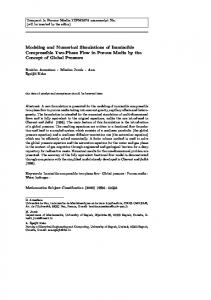
Figure 3.1. Structure of the approximate Riemann solver.
and � ) = (ρu, ρu2 + β, ρuv, (ρE + β)u, ρϕu, ρβu + u, ρcu, ρsu)T . F�(W c2 � such that the first five components of W � are exactly the components of W at the We choose W beginning of the time step. In addition, we have to set β, s and c and explain how we compute these aditional variables from the state W. In other words, we have to duplicate some variables computed from W at the beginning of the time step. The duplication has to be performed in such a way that the resulting solver is consistent with the exact one and that the whole scheme satisfies some stability properties. Thanks to the additional relaxed variables, the eigenvalues of the new system are linearly degenerated. Thus we can compute easily the exact solution to the relaxed Riemann problem. It has three wave speeds σ1 = u − ρc , σ2 = u, σ3 = u + ρc , with two intermediate states that we shall index by .1 and .2 (see Figure 3.1). We notice that c1 = cL and c2 = cR . Then, according to expression of the Riemann invariants for the first and thirth wave and the fact that u and β are two independant Riemann invariants for the central wave, the intermediate states are obtained by the relations
u1 = u2 , vL = v1 , sL = s1 , ϕL = ϕ1 , (β + uc)L = (β + uc)1 , β 1 β 1 ( + 2 )L = ( + 2 )1 , ρ c ρ c 2 β2 β (e − 2 )L = (e − 2 )1, 2c 2c
β1 = β2 , v2 = v R , s2 = sR , ϕ2 = ϕ R , (β − uc)2 = (β − uc)R , 1 β 1 β ( + 2 )2 = ( + 2 )R , ρ c ρ c 2 β β2 (e − 2 )2 = (e − 2 )R . 2c 2c
The wave speeds are given by
σ 1 = uL −
cL cR , σ 2 = u1 = u2 , σ 3 = uR + . ρL ρR
OPENCL NUMERICAL SIMULATIONS OF TWO-FLUID COMPRESSIBLE FLOWS WITH A 2D RANDOM CHOICE METHO
Then the solution is (3.15) (3.16) (3.17)
(3.18)
(3.19)
1 1 cR (uR − uL ) + βL − βR = + , ρ1 ρL cL (cL + cR ) 1 1 cL (uR − uL ) + βR − βL = + , ρ2 ρR cR (cL + cR ) βL − βR + cL uL + cR uR , u1 = u2 = cR + cL v1 = vL , v2 = vR , cL βR + cR βL + cL cR (uL − uR ) β1 = β2 = , cL + cR β2 − β2 e1 = eL − L 2 1 , 2cL 2 β − β2 e2 = eR − R 2 2 , 2cR ϕ1 = ϕL , ϕ2 = ϕR .
Of course, we have to relate the relaxed Riemann solver to our initial set of variables. In practice, as we already said, at the beginning of the time step, we duplicate the relaxed variables, which amounts to set (3.20) (3.21)
βL = p(ρL , eL , ϕL ), sL = s(ρL , eL , ϕL ),
βR = p(ρR , eR , ϕR ), sR = s(ρR , eR , ϕR ).
The objective is now to define proper cL and cR and the numerical flux in such a way that the Riemann solver satisfies good properties. We will study if our scheme is stable, it means that under some CFL condition, we have Win ∈ W for all i ⇒ Win+1 ∈ W for all i, where we denote by W the convex domain W = {(ρ, ρu, ρv, ρE, ρϕ)T : ρ ≥ 0; e = E −
u2 + v 2 ≥ 0}. 2
In order to study the stability of the scheme we will use the right and left numerical fluxes associated to the approximate Riemann solver of the extended system (3.13)-(3.14). These fluxes are defined by [11] (3.22)
(3.23)
�L , W �R ) = F�(W �L ) − F�L (W
ˆ0 −∞
�W �L , W �R , ω) − W �L )dω, (R(
ˆ+∞ �W �L , W �R , ω) − W �R )dω. �L , W �R ) = F�(W �R ) + (R( F�R (W 0
�L (W �L , W �R ) = F �R (W �L , W �R ) becomes The conservativity identity F
�1 − W �L ) + σ2 (W �2 − W �1 ) + σ3 (W �R − W �2 ) = F�(W �R ) − F�(W �L ). σ1 ( W
Conservativity thus enables to define the intermediate fluxes F�1 and F�2 by �L ) + σ1 (W �1 − W �L ), F�1 = F�(W �R ) − σ3 (W �R − W �2 ), F�2 = F�(W
OPENCL NUMERICAL SIMULATIONS OF TWO-FLUID COMPRESSIBLE FLOWS WITH A 2D RANDOM CHOICE METHO
which can be considered as a generalization of the Rankine-Hugoniot relations. The numerical flux of the extended system (3.13)-(3.14) is then given by �L ), F�(W � �L , W �R ) = F�L (W �L , W �R ) = F�R (W �L , W �R ) = F1 , F�(W F�2 , � � F (WR ),
if if if if
0 ≤ σ1 , σ1 ≤ 0 ≤ σ2 , σ2 ≤ 0 ≤ σ3 , σ3 ≤ 0.
The computation of the intermediate fluxes F�1 and F�2 gives us
u2 + v12 ρ1 β1 u1 F�1 = (ρ1 u1 , ρ1 u21 + β1 , ρ1 u1 v1 , (ρ1 (e1 + 1 ) + β1 )u1 , ρ1 u1 ϕ1 , + u1 , ρ1 c1 u1 , ρ1 s1 u1 )T , 2 c21 �1 ), = F�(W
u2 + v22 ρ2 β2 u2 F�2 = (ρ2 u2 , ρ2 u22 + β2 , ρ2 u2 v2 , (ρ2 (e2 + 2 + u2 , ρ2 c2 u2 , ρ2 s2 u2 )T , ) + β2 )u2 , ρ2 u2 ϕ2 , 2 c22 �2 ). = F�(W
It is remarkable that the intermediate numerical fluxes, which depends in the general cases on the left and right states, can be expressed as the flux of the corresponding intermediate state �L , W �R ) = F�(W �∗ ) for some W �∗ ∈ R8 ). of the relaxed system (i.e. F�(W This property is generally not true for the class of so-called “Godunov type finite volume schemes” as defined by Harten in [11]. For this class of schemes, the numerical flux is defined by integrating the approximate Riemann solver as in (3.22) and (3.23). And there is no reason that the numerical flux can be expressed in the form (3.12). The numerical flux F (WL , WR ) for the original system (3.1) is obtain by keeping only the first five components of our relaxed fluxes, we deduce F (WL ), F , 1 F (WL , WR ) = F2 , F (WR ),
(3.24)
where
if if if if
0 ≤ σ1 , σ1 ≤ 0 ≤ σ2 , σ2 ≤ 0 ≤ σ3 , σ3 ≤ 0,
u21 + v12 ) + β1 )u1 , ρ1 u1 ϕ1 )T , 2 u2 + v22 ) + β2 )u2 , ρ2 u2 ϕ2 )T . = (ρ2 u2 , ρ2 u22 + β2 , ρ2 u2 v2 , (ρ2 (e2 + 2 2
F1 = (ρ1 u1 , ρ1 u21 + β1 , ρ1 u1 v1 , (ρ1 (e1 + F2
Generally β1 �= p(ρ1 , e1 , ϕ1 ) and β2 �= p(ρ2 , e2 , ϕ2 ), and it is not possible to write the F (WL , WR ) = F (W ∗ ) for some W ∗ ∈ R5 . Remark: The positivity of ρ1 and ρ2 is not guaranteed from (3.15)-(3.16). This is a requirement that constraints cL and cR to be large enough. Another requirement is that σ1 < σ2 < σ3 , but indeed this property follows from the previous one, since one has σ2 − σ1 = cρL1 and σ3 − σ2 = cρR2 .
OPENCL NUMERICAL SIMULATIONS OF TWO-FLUID COMPRESSIBLE FLOWS WITH A 2D RANDOM CHOICE METHO
Property: In the Riemann problem (3.13)-(3.14) with initially (3.20) and (3.21), if ρL > 0 and ρR > 0, we define the relaxation speeds cL and cR by � ∂p cL ρ + uL − uR , 0), = ∂ρ (ρL , sL , ϕL ) + α max( � ∂ppR −pL L ρR ∂ρ (ρR ,sR ,ϕR ) if pR − pL ≥ 0, � cR = ∂p (ρR , sR , ϕR ) + α max( pL −pR + uL − uR , 0), ρR ∂ρ cL � ∂p ρcR = ∂ρ (ρR , sR , ϕR ) + α max( � ∂ppL −pR + uL − uR , 0), R ρL ∂ρ (ρL ,sL ,ϕL ) if pR − pL ≤ 0, � cL = ∂p (ρL , sL , ϕL ) + α max( pR −pL + uL − uR , 0), ρL ∂ρ cR
∂p then ∂ρ (ρ, s, ϕ) = γ(ϕ)sργ(ϕ)−1 . where α = max( γL2+1 , γR2+1 ), s = p+π ργ If we assume that the time step τn satisfies the CFL condition � τn · (σ1 )ni ≥ − h2 , (3.25) ∀ i τn · (σ2 )ni ≤ h2 ,
then, the Eulerian scheme (3.11) with the interface fluxes given by (3.24) has now the following properties (1) (2) (3) (4) (5)
it preserves the nonnegativity of ρ, it preserves the positivity of e, it satisfies discrete entropy inequalities for single fluid flows, stationnary contact discontinuities where u = 0, p = cst are exactly resolved, it handles data with vacuum.
For a proof, we refer to [5]1. In practice, we do not exactly apply the CFL condition (3.25). We rather compute a local time step (3.26)
τi,n =
h , 2 max(|(σ1 )ni | , |(σ3 )ni |)
and deduce an approximation of the stability time step (3.27)
τn = δ min τi,n , i
where δ is a safety factor, which satisfies 0 < δ < 1. The lagrangian scheme (3.7) can be treated in a similar way, in this case the interface flux is given by a formula that depends only on an intermediate state F (WL , WR ) = (0, β1 , 0, u1 β1 , 0)T = (0, β2 , 0, u2 β2 , 0)T , where β1 and u1 are given by the same formula (3.17)-(3.18). We can prove similarly at it was done in [5] that under the CFL condition (3.25) the Lagrangian scheme satisfies the properties 1, 2, 4 and 5 previously given. We are able to compute a Eulerian and a Lagrangian fluxes that have good properties. We have thus constructed an ALE flux too. Numerically, we have observed a excellent robustness of the Lagrange and projection scheme with the relaxation ALE flux. We were not able to construct a test case leading to a crash of the simulations. Of course, it is not easy to prove rigorously the stability and convergence of the scheme, because the projection step, which mixes deterministic and random averaging, is rather untypical. 1Actually
the proof has to be adapted, because we deal with two-fluid flows, but it is very similar.
OPENCL NUMERICAL SIMULATIONS OF TWO-FLUID COMPRESSIBLE FLOWS WITH A 2D RANDOM CHOICE METHO
1)&2()"*+*,
!"$
-."# !"/ !"0
-."$
%&'()"*+*,
!"#
%&'()"*+*,
1 .
3&45
Figure 4.1. A (virtual) GPU with 2 Compute Units and 4 Processing Elements 4. GPU and OpenCL implementation 4.1. OpenCL. For performance reasons, we decided to implement the 2D scheme on recent multicore processor architectures, such as a Graphic Processing Unit (GPU). Many different hardware exist, but schematically, a GPU can be considered as a device plugged into a computer, called a host. The device is made of (see Figure 4.1) • Global memory (typically 1 Gb2) • Compute units (typically 27). Each compute unit is made of: • Processing elements (typically 8). • Local (or cache) memory (typically 16 kb) The same program (a kernel) can be executed on all the processing elements at the same time, with the following rules: • All the processing elements have access to the global memory. • The processing elements have only access to the local memory of their compute unit. • If several processing elements write at the same location at the same time, only one write is succesful. • The access to the global memory is slow while the access to the local memory is fast. In order to operate a GPU, several tools are available. The CUDA environment, for instance, allows to drive the NVIDIA GPUs. OpenCL is a recent set of tools, which allow to program many kind of multicore processors, CPU or GPU. OpenCL means “Open Computing Language”. It includes: • A library of C functions, called from the host, in order to drive the GPU (or the multicore CPU); • A C-like language for writing the kernels that will be executed on the processing elements. OpenCL is practically available since september 2009 [16]. The specification is managed by the Khronos Group, which is also responsible of the OpenGL API design and evolutions. Virtually, 2the
typical values are given for a NVIDIA GeForce GTX 280 GPU
OPENCL NUMERICAL SIMULATIONS OF TWO-FLUID COMPRESSIBLE FLOWS WITH A 2D RANDOM CHOICE METHO
it allows to have as many compute units (work-groups) and processing elements (work-items) as needed. The threads are sent to the GPU thanks to a mechanism of command queues on the real compute units and processing elements. The main advantage of the OpenCL API is its portability. The same program can run on a multicore CPU or a GPU. Many resources are available on the web for learning OpenCL. For a tutorial and simple examples, see for instance [10]. 4.2. Implementation. We naturally organize the data in a (x, y) grid. In principle, the implementation is not very difficult because, thanks to the Strang splitting, the full algorithm is easy to parallelize. For recent GPU devices the number of compute units is of the order of several hundreds. This implies that the computations are very fast and that the time spent in the data memory transfers becomes the limiting factor. It is thus very important to well organize the data into memory. For instance, for computing the x-direction step (3.1), the data are well aligned into the memory and two successive processing elements access two neighbouring memories, which allows to achieve optimal memory bandwitdth (coalescing access). For the y-direction step (3.3), if nothing is done, two successive processing elements access different rows in memory, which leads to very slow memory access (typically ten times slower than the coalescing access!). Thus between the two steps, we have to perform an optimized transposition algorithm, described for instance in [19]. That said, the algorithm for one time step is rather simple: • we associate a processor to each cell of the grid. • we compute the stability time step for each cell i (see (3.26). If the local time step is lower than the global one, then we replace the global time step. This implies, in some cases, concurrent memory access to the global memory if two work-items modify together the time step. From the OpenCL norm, we know that exactly one access will be successful but we cannot know which (see Section 4.1). In order to avoid instabilities we decrease the global time step by an adequate safety factor. This approach is very simple but we cannot guarantee that all executions of our program on different devices will give exactly the same results. It would be possible to implement a parallel reduction algorithm for computing the time step [4], but it is a little bit more complicated and in practice our approach is very satisfactory. • we compute the fluxes balance in the x-direction for each cell of each row of the grid. A row (or a part of the row) is associated to one compute unit and one cell to one processor. As of october 2012, the OpenCL implementations generally imposes a limit (typically 1024) for the number of work-items inside a work-group. This forces us to split the rows for some large computations. • we employ a subdomain strategy in order to retain as much data as possible into the local cache memory of the work-group. When the rows are split, a covering of two cells is then necessary between the subdomain for ensuring the correctness at the boundary values. Indeed, the local cache memeory is not shared across work-groups. • we transpose the grid (exchange x and y) with an optimized memory transfer algorithm. • we compute the fluxes balance in the y-direction for each row of the transposed grid. Memory access are optimal. • we transpose again the grid. In Table 1, we compare our OpenCL code when it is run on one core or four cores of a multicore CPU, or on recent GPU. We observe spectacular speedups for the GPU simulations compared to the one-core simulation. The test case corresponds to the computation of 300 time steps of the algorithm on a 1024x512 grid. 5. Numerical results 5.1. One-dimensional results. Firstly, we present some numerical results on the one dimensional Euler equations (3.1) where we do not take into account the y-velocity, it means that
OPENCL NUMERICAL SIMULATIONS OF TWO-FLUID COMPRESSIBLE FLOWS WITH A 2D RANDOM CHOICE METHO
hardware time (s) speedup AMD A8 3850 (one core) 527 1 AMD A8 3850 (4 cores) 205 2.6 NVIDIA GeForce 320M 56 9.4 AMD Radeon HD 5850 3 175 AMD Radeon HD 7970 2 263 Table 1. Simulation times on different hardware Quantities Left Right −3 ρ (kg.m ) 10 1 −1 u (m.s ) 50 50 p (Pa) 1.1 × 10⁵ 1 × 10⁵ ϕ 1 0 γ 1.4 1.1 π 0 0 Table 2. Initial left and right states of the Riemann problem to illustrate the non convergence of the averaging projection.
v = 0 at any time. We compare different choices of projections for the lagrangian approach (see condition (3.7)). A classical choice is to use the averaging projection (3.9), the advantage of this projection is to obtain a conservative scheme but the problem is that the fraction of mass ϕ will be diffused. Indeed, the fourth equation of system (3.1) gives us the transport equation ∂t ϕ + u∂t ϕ = 0, then if at initial time we have ϕ ∈ 0, 1, theoricaly we have ϕ = 0 or ϕ = 1 at any time. With the averaging projection this is no more the case numerically and we have then to define mixture parameters law. In [20], it is given by 1 1 1 = ϕ + (1 − ϕ) , γ(ϕ) − 1 γ2 − 1 γ1 − 1 γ(ϕ)π(ϕ) γ 2 π2 γ 1 π1 = ϕ + (1 − ϕ) , γ(ϕ) − 1 γ2 − 1 γ1 − 1 where (γ1 , π1 ) and (γ2 , π2 ) correspond respectively to the pure liquid phase ϕ = 0 and the pure gas phase ϕ = 1 at the initial time. The resulting scheme has a very poor precision: for instance, if we consider the Riemann problem where the interface between the two fluids is located at time t0 = 0 s at position x = 1 m with the left and right states recorded in Table 2, we observe pressure oscillations for the numerical solution (see figure 5.1). Another approach is to consider the Glimm projection (3.10) in every cell. The resulting scheme is not conservative and in some case it does not converge. For instance, if we consider the Riemann problem where the interface between the two fluids is located at time t0 = 0 s at position x = 0 m. Left and right initial states are given in Table 3. A typical plot is given in Figure 5.2, where we compare the exact and the approximated densities at time t = 0.5 s. We also provide in Figure 5.3 a comparison of the two lagrangian schemes (mixed and averaging projection schemes) and the ALE scheme for the densities for a uniform mesh of 500 points. It is interesting to observe that the interface position is very well resolved (in only one mesh point) by the mixed projection scheme and the ALE scheme and that this good resolution of the contact wave also implies an improvement of the precision in the left rarefaction wave. The graph obtained with the mixed projection and with the ALE scheme seems to be superposed. In order to determine the less diffusive scheme we perform a convergence study. In Figure 5.4,
OPENCL NUMERICAL SIMULATIONS OF TWO-FLUID COMPRESSIBLE FLOWS WITH A 2D RANDOM CHOICE METHO 112000 ’p’ ’pex’ 110000
Pressure
108000
106000
104000
102000
100000 0
0.2
0.4
0.6
0.8
1 x
1.2
1.4
1.6
1.8
2
Figure 5.1. Oscillations on the pressure with the averaging projection for initial parameters recorded in Table 2. Quantities Left Right ρ (kg.m−3 ) 3.488 1 −1 u (m.s ) 1.13 −1 p (Pa) 23.33 2 ϕ 1 0 γ 2 1.4 π 7 0 Table 3. Initial left and right states of the Riemann problem to illustrate the non convergence of the Glimm projection.
Figure 5.2. Non convergence of the Glimm projection for initial parameters recorded in Table 3.
OPENCL NUMERICAL SIMULATIONS OF TWO-FLUID COMPRESSIBLE FLOWS WITH A 2D RANDOM CHOICE METHO
Figure 5.3. Comparison of the mixed and averaging projection schemes for initial parameters recorded in Table 3.
Figure 5.4. Convergence study in L1 norm for initial parameters recorded in Table 3. we compare the convergence in L1 norm of the different schemes: the ALE scheme is a little bit less diffuse that the mixed projection scheme. The convergence rate for the averaging projection is approximately 0.5, while it is 0.8 for the mixed projection and the ALE scheme.
OPENCL NUMERICAL SIMULATIONS OF TWO-FLUID COMPRESSIBLE FLOWS WITH A 2D RANDOM CHOICE METHO
t = 0 s.
t = 0.0067 s.
Figure 5.5. Inital place of the bubble on top left, final place of the bubble on the top right and zoom on the bubble interface on the bottom. 5.2. Pure convection. Now, we consider two-dimensional numerical tests for which we use the Strang dimensional splitting approach. The first test is to consider the convection of a spherical bubble of gas in a liquid phase. At time t = 0 the bubble is in the left top corner (see Figure 5.5). The initial parameters are presented in Table 4, the bubble moves to the bottom right corner. The results was performed with the ALE scheme and a uniform mesh of 512 × 512 points on the domain [0, 1] × [0, 1]. On this test case without pressure waves, the results are the same with the mixed projection scheme. The radius of the bubble is 0.1 m and the final time of computation is tf inal = 0.0067 s. For the boundary conditions, we impose the initial data at every time. As our algorithms do not diffuse the fraction of mass of gas ϕ, in fact ϕ = 1 in the bubble and ϕ = 0 outside the bubble at every time, we choose to plot ϕ to localize the bubble interface. We see in Figure 5.5 that the bubble moves correctly, the bubble at the final time is superimposed with the exact solution, which is plot in yellow dotted line. The last picture of the Figure 5.5 shows that the iterface bubble is not smooth. This lack of smoothness is of course due to the pseudo-random nature of the Glimm projection. 5.3. Test of Zalesak. Now, we consider another classical two dimensional numerical test. Firstly, we want to test dimensional splitting coupled with the Glimm projection. It is the test proposed by Zalesak [24] and consists of a computing the rotation of a complex solid shape. In
OPENCL NUMERICAL SIMULATIONS OF TWO-FLUID COMPRESSIBLE FLOWS WITH A 2D RANDOM CHOICE METHO
Quantities Inside the bubble Outside the bubble ρ (kg.m−3 ) 1.225 1000 −1 u (m.s ) 100 100 −1 v (m.s ) −75 −75 p (Pa) 1.01325 × 10⁵ 1.01325 × 10⁵ ϕ 1 0 γ 1.4 3 π 0 7.499 × 10⁸ Table 4. Inital datas for the test of a convected bubble. fact, we just solve the equation (5.1)
∂t ρ + ∂x (ρu) + ∂y (ρv) = 0,
where u = −Ω(y − y0 ) and v = Ω(x − x0 ). Here Ω is the constant angular velocity in rad/s and (x0 , y0 ) is the axis of rotation. In order to solve this equation we use the dimentional splitting, then we just precise the numerical scheme used to solve ∂t ρ + ∂x (ρu). In fact, we use the ALE numerical scheme hn+1,− ρn+1,− = hi ρni − ∆t(((ρu)i+1/2 − ζi+1/2 ρi+1/2 ) − ((ρu)i−1/2 − ζi−1/2 ρi−1/2 )), i i where ui+1/2 = (−Ω(y − y0 ))i+1/2 = −Ω(y − y0 ) does not depend on i (it just depends on y) and � ρi , if ui+1/2 < 0, ρi+1/2 = ρi+1 , if ui+1/2 ≥ 0. The domain is [0, 1] × [0, 1] and the solid considered is a cylinder of radius 0.15 m, through which a slot has been cut of witdth 0.05m. We assume that the density inside the cuted cylinder is ρ = 3 and outside we have ρ = 1. The rotational speed is chosen such that after 628 s the 2π cylinder will effect one complete revolution about the central point, i.e. Ω = 628 rad.s−1 . The results was performed with the ALE scheme and a uniform mesh of 1000 × 1000 points, the results were the same with the mixed projection scheme. The time step is chosen such that the quantity hin+1,− stay positive, we choose ∆t ≤
1 ∆x � . 2 max u2i + vi2 i
Remark: As we just consider the equation (5.1), the system is hyperbolic with only one wave speed σ = u then the CFL condition is less restrictive than for system (2.1). In Figure 5.6, we compare the shape of the cuted cylinder after different time. Features to be compared are the filling-in of the gap, erosion of the “bridge,” and the relative sharpness of the profiles decking the front surface of the cylinder. Even after 10 revolutions, the global aspect of the solid is preserved. The length of the “bridge” seems to be the same on the top and the bottom. The interface is not so badly solved, considering the simplicity of the Glimm approach, even if after 2 revolutions we observe that there are some part of the solid in the bridge. 5.4. Shock-droplet interaction. We now present a two-dimensional test that consists in simulating the impact of a Mach 1.22 shock travelling though air onto a cylinder of R22 gas. The shock speed is σ = 415 m.s−1 . This test aims at simulating the experiment of [12] and has been considered by several authors such as [17, 21, 15]. The initial conditions are depicted in Figure 5.7: a cylinder of R22 is surrounded by air within a Lx × Ly rectangular domain. At t = 0, the cylinder is at rest and its center is located at (X1 , Y1 ). We denote by r the initial
OPENCL NUMERICAL SIMULATIONS OF TWO-FLUID COMPRESSIBLE FLOWS WITH A 2D RANDOM CHOICE METHO
t = 0 s.
t = 314 s.( 12 revolution)
t = 628 s.(1 revolution)
t = 1256 s.(2 revolutions)
t = 3140 s.(5 revolutions)
t = 6280 s.(10 revolutions)
OPENCL NUMERICAL SIMULATIONS OF TWO-FLUID COMPRESSIBLE FLOWS WITH A 2D RANDOM CHOICE METHO
&*+) '"#
%$&#'() '"#$% ,--./0' *
!"#$% 1 2
Figure 5.7. Air-R22 shock/cylinder interaction test. Description of the initial conditions. Quantities Air (post-shock) Air (pre-shock) R22 −3 ρ (kg.m ) 1.686 1.225 3.863 u (m.s−1 ) −113.5 0 0 −1 v (m.s ) 0 0 0 p (Pa) 1.59 × 10⁵ 1.01325 × 10⁵ 1.01325 × 10⁵ ϕ 0 0 1 γ 1.4 1.4 1.249 π 0 0 0 Table 5. Air-R22 shock/cylinder interaction test. Initial data. radius of the cylinder. The planar shock is initially located at x = Ls and moves from right to left towards the cylinder. The parameters for this test are Lx = 445 mm, Ly = 89 mm, Ls = 275 mm, X1 = 225 mm, Y1 = 44.5 mm, r = 25 mm. Both R22 and air are modelled by two perfect gases whose coefficients γ and initial states are given in Table 5. The domain is discretized with a 5000 × 1000 regular mesh. Top and bottom boundary conditions are set to solid walls while we use constant state boundary conditions for the left and right boundaries. The shock reaches the R22 bulk after approximatively 60 µs. In the following we shall consider this time as the time origin t = 0. Figure 5.8 and Figure 5.9 display the evolution of the cylinder shape obtained with the ALE scheme and the experience of Hass and Sturtevant [12]. We can also compare our results to the computations of Kokh and Lagoutiere [15] because we consider the same test-case with the same initial datas. The profiles are obtained thank to the fraction of mass of gas ϕ: our scheme preserved ϕ = 1 in the gas and ϕ = 0 in the liquid. The overall location of the bulk is quite similar to the experimental results. The shape of the two vortices is not exactly the same on the top and the bottom, it comes from the random part of the Glimm projection. In fact, the Glimm projection in the y-direction use the velocity v and this velocity field is symetric with respect to the axis (O, x) where O is the center of the domain. 5.5. Shock-bubble. We perform another shock/interface interaction test proposed in [20, 15] that involves a gas bubble surrounded by a liquid. The geometry of the initial condition is
OPENCL NUMERICAL SIMULATIONS OF TWO-FLUID COMPRESSIBLE FLOWS WITH A 2D RANDOM CHOICE METHO
t = 55µs.
t = 115µs.
t = 135µs.
t = 187µs.
t = 247µs. Figure 5.8. Air-R22 shock cylinder interaction test. Pressure fied and interface on the left; experience of Hass and Sturtevant [12] on the right. depicted in Figure 5.7 with the following parameters values: Lx = 2 m, Ly = 1 m, Ls = 0.04 m, X1 = 0.5 m, Y1 = 0.5 m, r = 0.4 m. The gas within the bubble is governed by a perfect gas law while the liquid is modelled with the stiffened gas law. The EOS parameters and initial states are given in Table 6. The computation domain is discretized with a 3000×1000 grid and we use solid wall boundary conditions for the top and bottom boundaries, while we impose constant states at the left and right boundaries. The speed of the shock is σ = 10008 m.s−1 . Figure 5.11 and 5.12 display the mapping of respectively the density and the pressure at several instants. For the graph of pressure, as the maximum pressure increase with the time,
OPENCL NUMERICAL SIMULATIONS OF TWO-FLUID COMPRESSIBLE FLOWS WITH A 2D RANDOM CHOICE METHO
t = 318µs.
t = 342µs.
t = 417µs.
t = 1020µs. Figure 5.9. Air-R22 shock cylinder interaction test. Pressure fied and interface on the left; experience of Hass and Sturtevant [12] on the right. Quantities Liquid (post-shock) Liquid (pre-shock) Gas ρ (kg.m−3 ) 1030.9 1000.0 1.0 −1 u (m.s ) 300.0 0 0 −1 v (m.s ) 0 0 0 p (Pa) 3 × 10⁹ 105 105 ϕ 0 0 1 γ 4.4 4.4 1.4 π 6.8 × 10⁸ 6.8 × 10⁸ 0 Table 6. Liquid-gas/bubble interaction test. Initial data.
we can not use the same scale to plot all the graph: the first two graph are plot with different scales from the last two. As the difference of density inside and outside the bubble is huge, we can not see the shock position, but we can easily see the interface bubble by observing the density field. One can clearly see the important variation of the interface topology and more specially the creation of two symetrical vortices on each side of the axis (O, x) where O is the center the domain.
OPENCL NUMERICAL SIMULATIONS OF TWO-FLUID COMPRESSIBLE FLOWS WITH A 2D RANDOM CHOICE METHO
)*+,*.#(21("#
%$)*+,*./01("#
%$&'( /
!"#$% 3 4
Figure 5.10. Liquid-gas shock/bubble interaction test. Description of the initial conditions.
t = 225µs.
t = 225µs.
t = 375µs.
t = 375µs.
Figure 5.11. Liquid-gas/bubble interaction test. Density on the left and pressure fied on the right. Remark: At some times, we obtain negative pressures in the liquid. This is not a problem stays positive, indeed as p � −6 × 10⁶ Pa, γliquid = 4.4, because the internal energy e = p+γπ ρ πliquid = 6.8 × 10⁸ and ρ > 0 we obtain e > 0. 6. Conclusion We have proposed a new method for computing 2D compressible flows with interface. Our approach is based on a robust relaxation Riemann solver, coupled with a very simple random choice sampling projection at the interface. The properties of the resulting scheme are very interesting : • it preserves constant velocity and pressure states; • the mass fraction is not diffused at all; • it allows vacuum. In addition, the algorithm is easy to paralelize on recent multicore architectures. We have implemented the scheme in the OpenCL environment. The efficiency is spectacular: compared
OPENCL NUMERICAL SIMULATIONS OF TWO-FLUID COMPRESSIBLE FLOWS WITH A 2D RANDOM CHOICE METHO
t = 450µs.
t = 450µs.
t = 600µs.
t = 600µs.
Figure 5.12. Liquid-gas/bubble interaction test. Density on the left and pressure fied on the right. to a standard CPU implementation, we observed that the GPU computations are more than hundred times faster. References [1] Abgrall, Rémi How to prevent pressure oscillations in multicomponent flow calculations: a quasiconservative approach. J. Comput. Phys. 125 (1996), no. 1, 150–160. [2] M. Bachmann [3] Thomas Barberon, Philippe Helluy, and Sandra Rouy. Practical computation of axisymmetrical multifluid flows. Int. J. Finite Vol., 1(1):34, 2004. [4] Blelloch, G.E., Scans as Primitive Parallel Operations. IEEE Transactions on Computers, C38(11):1526–1538, November 1989. [5] Bouchut, François Nonlinear stability of finite volume methods for hyperbolic conservation laws and well-balanced schemes for sources. Frontiers in Mathematics. Birkhäuser Verlag, Basel, 2004. [6] C. Chalons, F. Coquel. Capturing infinitely sharp discrete shock pro- files with the Godunov scheme. Hyperbolic problems: theory, numer- ics, applications, 363–370, Springer, Berlin, 2008. [7] Coquel, Frédéric; Perthame, Benoît Relaxation of energy and approximate Riemann solvers for general pressure laws in fluid dynamics. SIAM J. Numer. Anal. 35 (1998), no. 6, 2223–2249 [8] Thierry Gallouët, Jean-Marc Hérard, and Nicolas Seguin. A hybrid scheme to compute contact discontinuities in one-dimensional Euler systems. M2AN Math. Model. Numer. Anal., 36(6) :1133–1159 (2003), 2002. [9] C. Chalons, P. Goatin. Transport-equilibrium schemes for computing contact discontinuities in traffic flow modeling. Commun. Math. Sci., 5 (2007), no. 3, 533–551. [10] Crestetto A., Helluy P. An OpenCL tutorial. 2010. http://www-irma.u-strasbg.fr/~helluy/ OPENCL/tut-opencl.html [11] A. Harten, P. D. Lax, and B. Van Leer. On upstream differencing and Godunov-type schemes for hyperbolic conservation laws. SIAM Rev., 25(1) :35–61, 1983. [12] J. F. Hass and B. Sturtevant. Interaction of weak shock waves with cylindrical ans spherical gas inhomogeneities. J. Fluid Mechanics, 181, 41-71, 1997. [13] Mathieu Bachmann, Philippe Helluy, Jonathan Jung, Hélène Mathis, Siegfried Müller. Random sampling remap for compressible two-phase flows, 2011, submitted. Preprint at http: //hal.archives-ouvertes.fr/hal-00546919 [14] Karni, Smadar Multicomponent flow calculations by a consistent primitive algorithm. J. Comput. Phys. 112 (1994), no. 1, 31–43. [15] S. Kokh, F. Lagoutière. An anti-diffusive numerical scheme for the simulation of interfaces between compressible fluids by means of the five-equation model. J. Computational Physics, 229, 2773-2809, 2010. [16] Khronos Group. OpenCL online documentation. http://www.khronos.org/opencl/ [17] J. J. Quirk and S. Karni. On the dynamics of a shock-bubble interaction. J. Fluid Mechanics, 318, 129-163, 1996.
OPENCL NUMERICAL SIMULATIONS OF TWO-FLUID COMPRESSIBLE FLOWS WITH A 2D RANDOM CHOICE METHO
[18] P. L. Roe. Approximate Riemann solvers, parameter vectors, and difference schemes. J. Comput. Phys., 43(2) :357–372, 1981. [19] Ruetsch, G., Micikevicius, P. Optimizing Matrix Transpose in CUDA. NVIDIA GPU Computing SDK, 1 – 24. 2009. [20] R. Saurel, R. Abgrall. A simple method for compressible multifluid flows. SIAM J. Sci. Comput., 21 (3), 1115-1145, 1999. [21] K. M. Shyue. A wave-propagation based volume tracking method for compressible multicomponent flow in two space dimensions. J. Comput. Phy., 215, 219-244, 2006. [22] Strang, Gilbert On the construction and comparison of difference schemes. SIAM J. Numer. Anal. 5 1968 506–517. [23] E. F. Toro. Riemann solvers and numerical methods for fluid dynamics, 2nd edition. Springer, 1999 [24] Fully Multidimensional Flux-Corrected Algorithms for Fluids. J. Computational Physics, 31, 335362, 1969.
IRMA, Université de Strasbourg, 7 rue Descartes, 67000 Strasbourg, France,
[email protected] [email protected]