the introduction of the first version of Microsoft KinectTM, shown in Fig. 2.1, based ..... is a cuboidal window W.p/ ma
Chapter 2
Operating Principles of Structured Light Depth Cameras
The first examples of structured light systems appeared in computer vision literature in the 1990s [5–8, 20] and have been widely investigated since. The first consumergrade structured light depth camera products only hit the mass market in 2010 with the introduction of the first version of Microsoft KinectTM , shown in Fig. 2.1, based on the PrimesensorTM design by Primesense. The Primesense design also appeared in other consumer products, such as the Asus X-tion [1] and the Occipital Structure Sensor [3], as shown in Fig. 2.2. Primesense was acquired by Apple in 2013, and since then, the Occipital Structure Sensor has been the only structured light depth camera in the market officially based on the Primesense design. Recently, other structured light depth cameras reached the market, such as the Intel RealSense F200 and R200 [2], shown in Fig. 2.3. As explained in Sect. 1.3, the configuration of structured light systems is flexible. Consumer depth cameras can have a single camera, as in the case of Primesense products and the Intel F200, or two cameras, as in the case of the Intel R200 (and of the so called space-time stereo systems [9, 22], which will be shown later to belong in the family of structured light depth cameras). This chapter, following the approach of Davis et al. [9], introduces a unified characterization of structured light depth cameras in order to present existing systems as different members of the same family. The first section of this chapter introduces camera virtualization, the concept that the presence of one or more cameras does not introduce theoretical differences in the nature of the measurement process. Nevertheless, the number of cameras has practical implications, as will be seen. The second section provides various techniques for approaching the design of the illuminator. The third section examines the most common non-idealities one must take into account for the design and usage of structured light systems. The fourth section discusses the characteristics of the most common commercial structured light systems within the introduced framework.
© Springer International Publishing Switzerland 2016 P. Zanuttigh et al., Time-of-Flight and Structured Light Depth Cameras, DOI 10.1007/978-3-319-30973-6_2
43
44
2 Operating Principles of Structured Light Depth Cameras
Fig. 2.1 Microsoft KinectTM v1
Fig. 2.2 Products based on the Primesense design: structure sensor by Occipital (left) and Asus X-tion Pro Live (right)
Fig. 2.3 Intel RealSense F200 (left) and R200 (right)
2.1 Camera Virtualization In order to introduce the camera virtualization concept, consider Fig. 2.4, in which pA is projected on three surfaces at three different distances: z1 , z2 and z3 . For each distance zi , according to (1.8), the point is framed by C at a different image location pC;i D ŒuC;i ; vC � with vC D vA and uC;i D uA C di with disparity di D bf =zi , in which b is the baseline of the camera-projector system and f is the focal length of the camera and the projector (since they coincide in the case of a rectified system) expressed in pixel units. The disparity of each pixel pCi can be expressed as a disparity difference or relative disparity with respect to a selected disparity reference. In particular, if the selected disparity reference is dREF D d2 , the values of d1 and d3 can be expressed
2.1 Camera Virtualization
45
P3 P2 P1
uC
uA
vC
vA
C
pA
A
IC Epipolar line
pC1 pC2 pC3
Fig. 2.4 The ray of the projected pattern associated with pixel pA intersects the scene surface at points P1 , P2 and P3 placed at different distances, and is reflected back to pixels pC1 , pC2 and pC3 of the image acquired by the camera
with respect to d2 as signed difference dREL1 D d1 � d2 and dREL3 D d3 � d2 . Given the value of zREF D z2 and of dREL1 and dREL3 , the value of z1 and of z3 can be computed as �zi D
1 � z2 1 dRELi C z2 bf
zi D z2 C �zi ;
(2.1)
i D 1; 3:
Equation (2.1) shows how to compute the scene depth zi for every pixel pCi of the camera image IC from a reference depth zREF and relative disparity values dRELi , taken with respect to the reference disparity value dREF (dREF D d2 in our example). Note that if the absolute disparity range for the structured light system is Œdmin ; dmax �, generally with dmin D 0 (and definitely with dmin � 0) the relative disparity range with respect to the reference disparity dREF becomes ŒdRELmin ; dRELmax � D Œdmin � dREF ; dmax � dREF �. Also, while relative disparity dREL is allowed to be negative, its absolute counterpart d is strictly non-negative in accordance to the rules of epipolar geometry. The generalization of the idea behind the above example leads to the so called camera virtualization i.e., a procedure hinted in [9], by which a structured light depth camera made by a single camera and an illuminator operates equivalently to a structured light depth camera made by two rectified cameras and an illuminator.
46
2 Operating Principles of Structured Light Depth Cameras
Fig. 2.5 Illustration of the reference image usage: (left) The structured light system, in front of a flat surface at known distance zREF ; (middle) reference image and computation of dREF from zREF ; (right) generic scene acquired with pixel coordinates referring to the reference image coordinates
Camera virtualization, schematically shown in Fig. 2.5, assumes a reference image IREF concerning a plane at known reference distance zREF . The procedure requires one to associate each point pREF with coordinates pREF D ŒuREF ; vREF �T of IREF to the corresponding point p of image IC acquired by camera C and to express its coordinates with respect to those of pREF , as p D Œu; v�T D ŒuREF C dREL ; vREF �. In this way the actual disparity value d of each scene point given by (1.16) can be obtained by adding dREF to the relative disparity value dREL directly computed from the acquired image IC , i.e., d D dREF C dREL :
(2.2)
Furthermore, from (1.17) and (2.2), comparison uC D uA C d uREF D uA C dREF
(2.3)
gives uC � uREF D d � dREF D dREL
(2.4)
uREF D uC � dREL :
(2.5)
or
2.1 Camera Virtualization
47
Equation (2.5) has the same structure of (1.16) and is the desired result, since it indicates that single camera light systems like the one in Fig. 2.4 operate identically to standard stereo systems with a real acquisition camera C as the left camera and a “virtual” camera C0 as the right camera co-positioned with the projector. Camera C0 has the same intrinsic parameters of camera C. The same conclusion can be reached less formally but straightforwardly by just noting that the shifting of reference image IREF by its known disparity value dREF gives an image which would be acquired by a camera C0 with the same characteristics of C, co-positioned with the projector. With respect to the reference image, depending whether the projector projects one or more patterns, the reference representation IREF may be made by one or more images. In order to be stored in the depth camera memory and used for computing the disparity map at each scene acquisition, the reference image IREF can be either acquired by an offline calibration step or just computed by a virtual projection/acquisition based on the mathematical model of the system. Direct acquisition of reference image IREF represents an implicit and effective way of avoiding non-idealities and distortions due to C and A and their relative placements. A calibration procedure meant to accurately estimate the position of the projector with respect to the camera by a set of acquisitions of a checkerboard with the projected pattern superimposed is provided by Zhang et al. [21]. The advantage of a reference image IREF generated by a close-form method due to a mathematical projection/acquisition model is that it does not need to be stored in memory and may be re-computed on-the-fly as in the case of a temporal pattern in which the coordinates of each pixel are directly encoded into the pattern itself. Camera virtualization plays a fundamental conceptual role since it decouples the structured light system geometry from the algorithms used on them: in other words, standard stereo algorithms can be applied to structured light systems whether they have one or two cameras, unifying algorithmic methods for passive and active methods independently from the geometric characteristics of the latter. A natural question prompted by the above observation is, given the complete operational equivalence between single camera and double camera systems, why should one use two cameras instead of one? The reason is that, although the presence of a second physical camera may seem redundant, in practice it leads to several system design advantages. The existence on the market of both single camera and two cameras systems is an implicit acknowledgment of this fact. For instance, the Intel RealSense F200 and the Primesense cameras belong to the first family, while the Intel RealSense R200 camera belongs to the second family. The usage of two cameras leads to better performance because it simplifies the handling of many system non-idealities and practical issues, such as the distortion of the acquired pattern with respect to the projected one due to camera and projector non-idealities and to their relative alignment. Furthermore, in order to benefit from the virtual camera methodology, the projected pattern should maintain the same geometric configuration at all times. This requirement can be demanding for camera
48
2 Operating Principles of Structured Light Depth Cameras
Wrong disparities percentage
Wrong disparities percentage function of image noise 3.5
S2 S1
3 2.5
Typical camera noise value
2 1.5 1 0.5 0 5
10
15
20
25
30
35
40
45
50
Image noise
Noise: s = 5
Noise: s = 30
Noise: s = 50
Fig. 2.6 Simulation of the performance of a single camera structured light system projecting the Primesense pattern (S1) and of a double-camera structured light system projecting the Primesense pattern (S2) for a flat scene textured by the “Cameraman” image at various noise levels
systems with an illuminator based on laser technology, because the projected pattern tends to vary with the temperature of the projector. For this reason, an active cooling system is used in the Primesense single camera system design, while it is unnecessary in the two cameras Intel RealSense R200. Another fundamental weakness of single camera systems is that any ambient illumination at acquisition time leads to a difference between the appearance of the acquired representation and that of the reference representation. This effect, most evident in outdoor scenarios, can be exemplified by the following simulation with a test scene made by a flat wall textured by an image, e.g., the standard “Cameraman” of Fig. 2.6. This scene offers a straightforward depth ground truth which is a constant value everywhere if the structured light system is positioned in a fronto-parallel situation with respect to the wall (i.e., if the optical axis of the rectified system cameras and projector are assumed orthogonal to the wall). At the same time the scene texture helps the selection of matching points in stereo algorithms. With respect to the above scene, let us computationally simulate a structured light system projecting the Primesense pattern with a single acquisition camera, like in commercial products, and a structured light system projecting the
2.1 Camera Virtualization
49
Primesense pattern but carrying two acquisition cameras instead of just one. For simplicity we will call S1 the former and S2 the latter. As a first approximation, the scene brightness can be considered proportional to the reflectance and illumination made by a uniform component (background illumination) and by a component due to the Primesense pattern. In the case of S1, in order to mimic camera virtualization we consider two acquisitions of a shifted version of “Cameraman”, while in S2 we consider only one acquisition per camera, and compare them with respect to the actually projected pattern. The acquisitions with S1 and S2 are repeated using versions of the “Cameraman” images corrupted by independent additive Gaussian noise with different standard deviations. Determining which of the two systems performs a better disparity estimation can be easily ascertained from the percentage of non constant, i.e., wrong depth values (in this case produced by a block-matching stereo algorithm with window size 9 � 9) as a function of the independent additive Gaussian camera noise, as shown in Fig. 2.6 for S1 and S2. The performance of the depth estimation procedure of S1 (red) is worse than the one of S2 (blue), especially for typical camera noise values (green line). In spite of its simplicity, this simulation provides an intuitive understanding of the approximations associated with the presented camera virtualization technique. In order to cope with the above mentioned illumination issues, single camera structured light systems adopt a notch optical filter on the camera lenses with a band-pass bandwidth tightly matched to that of the projected pattern. Moreover, in the case of extremely high external illumination in the projector’s range of wavelengths, a double camera structured light depth camera can be used as a standard stereo system, either by neglecting or switching off the contribution of the active illuminator A. For both a physical or virtual second camera, the disparity estimation with respect to the reference image IREF corresponds to a computational stereopsis procedure between two rectified images [16, 18]. Given this, one can continue to use local algorithms, i.e., methods which consider a measure of the local similarity (covariance) between all pairs of possible conjugate points on the epipolar line and simply select the pair that maximizes it, as observed in Sect. 1.2. The global methods mentioned in Sect. 1.2.1.3 that do not consider each couple of points on their own but exploit global optimization schemes are generally not used with structured light systems. From now on, in light of all the considerations provided about camera virtualization, this book will only consider structured light depth cameras made by two cameras and an illuminator, with the understanding that any reasoning presented in the remainder of the book also applies to the case of single camera structured light systems.
50
2 Operating Principles of Structured Light Depth Cameras
2.2 General Characteristics Let us refer for simplicity to the single camera structured light system of Fig. 1.11 in order to recall the operation of structured light systems: each pixel of the projector is associated with a specific local configuration of the projected pattern called code word. The pattern undergoes projection by A, reflection by the scene and capture by C. A correspondence algorithm analyzes the code words received by the acquired image IC in order to compute the conjugate pc of each pixel pA of the projected pattern. The goal of pattern design (i.e., code word selection) is to adopt code words effectively decodable even in the presence of non-idealities of the pattern projection/acquisition process pictorially indicated in Fig. 1.11 and explained in the next section. Figure 2.7 shows an example of the data acquired by a single camera structured light system projecting the Primesense pattern. The data acquired by a structured light depth camera are: • the images IC and IC0 acquired by cameras C and C0 , respectively, defined on the lattices �C and �C0 associated with cameras C and C0 . The axes that identify �C coincide with uC and vC of Fig. 1.11. The axes of �C0 will similarly refer to those of u0C and vc0 on the virtual or actual camera C0 . The values of IC and IC0 belong to interval Œ0; 1�. Images IC and IC0 can be considered a realization of the random fields IC and IC0 defined on �C and �C0 , with values in Œ0; 1�. In single camera structured light systems, like in the case of the Primesense depth camera, C0 is a virtual camera, and the image IC0 is not available. The data available at the output of a structured light depth camera are: O C , is defined on the lattice �C associated • The estimated disparity map, called D O with the C sensor. The values of DC belong to interval Œdmin ; dmax �, where dmin and OC dmax are the minimum and maximum allowed disparity values. Disparity map D can be considered a realization of a random field DC defined on �C , with values in Œdmin ; dmax �. O C , called ZO C , is • The estimated depth map computed by applying (1.26) to D defined on the lattice �C associated with camera C. The values of ZO C belong to the interval Œzmin ; zmax �, where zmin D bf =dmax and zmax D bf =dmin are the
O C and ZO C acquired by the Primesense depth camera Fig. 2.7 Example of IC , D
2.2 General Characteristics
51
minimum and maximum allowed depth values, respectively. Depth map ZO C can be considered as a realization of a random field ZC defined on �C , with values in Œzmin ; zmax �.
2.2.1 Depth Resolution Since structured light depth cameras are based on triangulation, they have the same depth resolution model as that of standard stereo systems. In particular, their depth resolution �z can be computed as �z D
z2 �d bf
(2.6)
where �d is the disparity resolution. Equation (2.6) shows that the depth resolution is quadratically dependent on the depth of the measured object (i.e., its z coordinate). Disparity resolution �d can be 1 in the case of pixel resolution or less than 1 in the case of sub-pixel resolution. Techniques for sub-pixel disparity estimation are well-known in stereo literature [16, 18] and they can also be applied to structured light systems. For example, according to the analysis of Konoldige and Mihelich [11], the KinectTM v1 uses a sub-pixel refinement process with interpolation factor 8, hence �d D 1=8, and according to [17] with baseline b D 75 [mm] and focal length approximately f D 585:6 [pxl]. Figure 2.8 shows a plot of the depth resolution of a system with the same parameters as those of KinectTM v1 and various sub-pixel precisions.
Depth Resolution
Depth resolution [mm]
100
Subpixel 1/16 Subpixel 1/8 Subpixel 1/4
80 60 40 20 0
0
500
1000
1500
2000
2500
3000
3500
4000
Distance [mm] Fig. 2.8 Depth resolution according to (2.6) for systems with baseline b D 75 [mm] focal length f D 585:6 [pxl] and sub-pixel precisions: �d D 1=16, 1=8 and 1=4
52
2 Operating Principles of Structured Light Depth Cameras
2.3 Illuminator Design Approaches The objective of structured light systems is to simplify the correspondence problem through projecting effective patterns by the illuminator A. This section reviews current pattern design methodologies. In addition, the specific design of the illuminator as well as its implementation are at the core of all structured light depth cameras. A code word alphabet can be implemented by a light projector considering that it can produce nP different illumination values called pattern primitives (e.g., nP D 2 for a binary black-and-white projector, nP D 28 for a 8-bit gray-scale projector, and nP D 224 for a RGB projector with 8-bit color channels). The local distribution of a pattern for a pixel pA is given by the illumination values of the pixels in a window around pA . If the window has nW pixels, there are nnPW possible pattern configurations on it. From the set of all possible configurations, N configurations need to be chosen as code words. What is projected to the scene and acquired by C is the pattern resulting from the code words relative to all the pixels of the projected pattern. Let us assume that the projected pattern has NRA � NCA pixels piA , i D 1; : : : ; NRA � NCA where NRA and NCA are the number of rows and columns of the projected pattern, respectively. The concept of pattern uniqueness is an appropriate starting point to introduce the various approaches for designing illuminator patterns. Consider an ideal system in which images IC and IC0 are acquired by a pair of rectified cameras C and C0 (whether C0 is real or virtual is immaterial for the subsequent discussion) and assume the scene to be a fronto-parallel plane corresponding to disparity 0 at infinity and infinite reflectivity. Since the cameras are rectified, let us recall from Sect. 1.2 that conjugate points p and p0 , i.e., points of IC and IC0 corresponding to the same 3D point P, are characterized by coordinates with the same v-component and ucomponents differing by disparity d: p D Œu; v�T , p0 D Œu0 ; v 0 �T D Œu � d; v�T . The correspondences matching process searches the conjugate of each pixel p in IC , by allowing d to vary in the range Œdmin ; dmax � and by selecting the value dO for which the local configuration of IC around p is most similar to the local configuration of IC0 around p � Œd; 0�T according to a suitable metric. Images IC and IC0 can carry multiple information channels, for instance encoding data at different color wavelengths (e.g., R, G, B channels) or at multiple timestamps t D 1; : : : ; N with N being the timestamp of the most recent frame acquired by cameras C and C0 . The local configuration in which the images are compared is a cuboidal window W.p/ made by juxtaposing windows centered at p in the different channels. If there is only one channel (with respect to time), the system is characterized by an instantaneous behavior and is called a spatial stereo system, according to [9]. On the contrary, if the matching window is characterized by a single-pixel configuration in the image (e.g., the window is only made by the pixel with coordinate p) and by multiple timestamps, the system is called a temporal stereo system. If the matching window has both a spatial and temporal component, the system is called space-time stereo. A standard metric to compute the local
2.3 Illuminator Design Approaches
53
similarity between IC in the window W.p/ and IC0 in the window W.p0 / is the Sum of Absolute Differences (SAD) of the respective elements in the two windows, defined as X SADŒIC .W.p//; IC0 .W.p0 //� , jIC .q/ � IC0 .q0 /j: (2.7) q2W.p/;q0 2W.p0 /
Since generally the windows W on which the SAD metric is computed are predefined, the value of the SAD metric is fully specified from p and d, as emphasized by notation SADIC ;IC0 ;W .p; d/ , SADŒIC .W.p//; IC0 .W.p0 //�
(2.8)
rewritten for simplicity just as SAD.p; d/. For each pixel p one selects the disparity O that minimizes the local similarity as d.p/ D argmin SAD.p; d/. A pattern is said to be unique if in an ideal system, i.e., a system without any deviation from theoretical behavior, for each pixel p in the lattice of IC , the value of the SAD metric of the O actual estimated disparity d� coincides with minimum d.p/ D argmin SAD.p; d/, which is unique. The uniqueness U of a pattern is defined as U , min U.p/ p2�C
(2.9)
where U.p/ is computed as the second argmin of the SAD metric, excluding the first O argmin d.p/ and the values within one disparity value from it, i.e., O O O d 2 fdmin ; : : : ; dmax g X fd.p/ � 1; d.p/; d.p/ C 1g:
(2.10)
Let us further comment on the above definition of uniqueness. For each pixel in the image IC the uniqueness map U.p/ is computed as the cost of the non-correct match that gives the minimum matching error. The higher such cost is, the more robust the pattern is against noise and non-idealities. The minimum uniqueness value across the entire pattern is selected in order to obtain a single uniqueness value for the entire pattern. This enforces the fact that the pattern should be unique everywhere in order to obtain a correct disparity estimation for each pixel, at least in the case of ideal acquisition. The minimum value of uniqueness for a pattern is 0. If a pattern has uniqueness greater than 0, it means that the pattern itself makes the conjugate correspondence detection problem a well-posed problem for each pixel in the pattern, otherwise the correspondence detection is ill-posed, at least for a certain number of pixels in the pattern. In the above discussion, uniqueness was defined using SAD as a matching cost function, but uniqueness can be defined in terms of other types of metrics or matching costs, such as the Sum-of-Squared-Differences (SSD), Normalized Cross-Correlation (NCC), or the Hamming distance of the Census transform [20].
54
2 Operating Principles of Structured Light Depth Cameras
The choice of matching cost is generally system dependent. For simplicity’s sake, in the rest of this book all uniqueness analysis will refer to standard SAD defined by (2.7).
2.3.1 Implementing Uniqueness by Signal Multiplexing The just-defined concept of uniqueness is a function of the number of color channels, the range of values in the image representation, and the shape of the matching window, which may have both a spatial and temporal component. Following the framework of Salvi et al. [15], different choices of these quantities lead to different ways to encode the information used for correspondences estimation, typically within the following four signal multiplexing families: • • • •
wavelength multiplexing; range multiplexing; temporal multiplexing; spatial multiplexing.
Each multiplexing technique performs some kind of sampling in the information dimension typical of the technique, limiting the reconstruction capability in the specific dimension. This concept is instrumental in order to understand the attributes of different structured light depth cameras according to the considered multiplexing techniques.
2.3.1.1
Wavelength Multiplexing
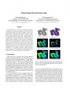
If the projected pattern contains light emitted at different wavelengths, i.e., different color channels, the system is characterized by wavelength-multiplexing. An example is a system with an illuminator projecting red, green, and blue light. Today, there is no commercial structured light depth camera implementing a wavelength multiplexing strategy, but such cameras have been widely studied, for instance in [10] and in [21]. Figure 2.9 shows an image of the projected pattern from [21]. This type of technique makes strong assumptions about the characteristics of the cameras and the reflectance properties of the framed scene. Notably, it assumes the
Fig. 2.9 Example of pattern projected by the illuminator of Zhang et al. (center) on a scene characterized by two hands (left), and the relative depth estimate (right). Courtesy of the authors of [21]
2.3 Illuminator Design Approaches Fig. 2.10 Schematic representation of “direct coding”, special case of wavelength multiplexing
55
Projected pattern
pA
Associated code-word
Pixel pA
pA
camera pixels that collect different channels are not affected by inter-channel crosstalk, which is often present. In addition, the scene is assumed to have a smooth albedo distribution without abrupt reflectivity discontinuities. For an analysis of these assumptions, the interested reader is referred to [21]. Since wavelength-multiplexing approaches sample the wavelength domain, in general they limit the capability of the system to deal with high frequency reflectivity discontinuities at different wavelengths. Therefore, the depth estimates produced by these types of systems tend to be correct for scenes with limited albedo variation and external illumination, but not in other cases. In direct coding [15] each pixel within a scanline is associated with a specific color value, as schematically shown in Fig. 2.10. Hence, direct coding is a special case of wavelength multiplexing where the disparity of a pixel can be estimated by matching windows of size 1. In general, combining different multiplexing techniques together leads to more robust systems. An example of a system combining wavelength and temporal multiplexing techniques is described in [21].
2.3.1.2
Range Multiplexing
In the case of a single channel, the projected pattern range can be either binary (black or white, as in Primesense products or in the Intel RealSense F200) or characterized by multiple gray level values (as in the Intel RealSense R200). The case of range characterized by multiple gray levels is usually referred as range multiplexing. Figure 2.11 shows the pattern of the Intel RealSense R200, which uses a range multiplexing approach. Figure 2.17 compares the textured pattern produced by the Intel RealSense R200 with the pattern of the Primesense camera, which uses binary dots instead of range multiplexing.
56
2 Operating Principles of Structured Light Depth Cameras
(a)
(b)
Fig. 2.11 Pattern projected by the Intel RealSense R200 camera: (a) full projected pattern; (b) a zoomed version of a portion of the pattern
Even though range multiplexing has interesting properties, it has not received as much attention as other multiplexing methods. In particular, range multiplexing does not require collimated dots, thus avoiding eye safety issues. Projecting grayscale texture allows one to gather more information in the matching cost computation step, in particular with some stereo matching techniques [20]. However, since image acquisition is affected by noise and other non-idealities, the local differences in the images may not exactly reflect the local differences of the projected pattern and such appearance difference may not be the same in the images IC and IC0 of the two cameras. Therefore, the range multiplexing information is at risk of being hidden by the noise and non-idealities of the camera acquisition process. Since range multiplexing samples the range of the projected pattern and of the acquired images, it limits the system’s robustness with respect to the appearance non-idealities which may differ for the two cameras, especially in low SNR situations. A major issue of range multiplexing is that different pixels of the projected texture have different illumination power. Consequently, dark portions of the pattern are characterized by lower power than bright areas. Combined with the fact that the optical power of the emitted pattern decreases with the square of the distance of the framed scene, it is not possible to measure far distances in correspondence to the dark areas of the pattern. Different from the case of wavelength multiplexing, direct coding alone becomes impractical in the case of range multiplexing, as shown by the following example. Consider the case of a disparity range made by 64 disparities, where the projector uses 64 range values and the acquired image range, encoded with 8 bits, has 256 values. If one adopted “direct coding,” the system would be robust to non-idealities up to 2 range values. Since the standard deviation of the thermal noise of a typical camera is in the order of 5–10 range values, the noise resilience of “direct coding” in the case of range multiplexing would clearly be inadequate. For this reason, range
2.3 Illuminator Design Approaches
57
multiplexing is typically used in combination with other multiplexing techniques, such as spatial multiplexing, as in the case of the Intel RealSense R200 camera.
2.3.1.3
Temporal Multiplexing
Temporal multiplexing is a widely investigated technique originally introduced for still scenes [19] and subsequently extended to dynamic scenes in [22], where the illuminator projects a set of N patterns, one after the other. The patterns are typically made by vertical black and white stripes representing the binary values 0 and 1, as shown in Fig. 2.12 for N D 3, since in this case there is no need to enforce wavelength or range multiplexing as the system is assumed rectified. This arrangement at time N ensures a different binary code word of length N for each line pixel pA ; all the rows have the same code words given the vertical symmetry of the scheme. The total number of available code words is 2N . In the case of acquisition systems made by a pair of real cameras, this method is typically called space-time stereo. For a comprehensive description of temporal multiplexing techniques see [15], while for details on space-time stereo see [9, 22]. The first example of a commercial camera for dynamic scenes based on temporal multiplexing was the Intel RealSense F200 camera. Figure 2.13 shows an example of projected patterns and acquired images for space-time stereo system.
0
0 0
0
1
1
1 1
pA
t= 1
0
0 1
1
0
0
1 1
t
pA
t= 2
pA
0
1 1 0
1 0
1
0
1
0 1
pA
t= 3
pA
Fig. 2.12 Temporal multiplexing: vertical black and white stripes coding a pattern at multiple timestamps (with N D 3)
58
2 Operating Principles of Structured Light Depth Cameras
Fig. 2.13 Example of projected patterns and acquired images for temporal multiplexing
The critical component of temporal multiplexing is the method used in order to create the set of projected patterns. As described in [15], there exist several pattern design techniques. The most popular is one based on Gray codes. In Gray codes, each code word differs from the previous one by just one bit. If the length of the code word is N, it is possible to generate exactly 2N uniquely decodable code words of a Gray code by the scheme pictorially shown in Fig. 2.14. In order to have a pattern with more values than the number of code words, it is possible to stack the patterns side by side. If 2N is greater than the maximum disparity that the system can measure, the produced code maintains its uniqueness property. Note that this assumes there is one pixel of the projected pattern for each pixel of the acquired images. This hypothesis usually holds for well-engineered systems, but if not verified, one should adjust the reasoning in order to account for the specific properties of the system. As suggested in [22], projected patterns for temporal multiplexing techniques should be characterized by high spatial frequency. However, as shown in Fig. 2.14, spatial frequencies differ for each pattern and increase for the bottom patterns. In order to address this issue and improve the performance of Gray coded patterns, the authors of [22] suggest shuffling the columns of the projected patterns as shown in Fig. 2.15 for N D 7. Note that the same shuffling sequence must be applied to all the patterns in order to preserve the uniqueness property characteristic of the Gray pattern. Another popular variation of Grey coding includes a post-refinement based on phase-shifting.
2.3 Illuminator Design Approaches
59
Fig. 2.14 Example of patterns for temporal multiplexing generated with Gray code, with code word length N D 7 suited to distinguish between 128 disparity levels
Fig. 2.15 Example of patterns obtained by permuting a Gray code with code word length N D 7 suited to distinguish between 128 disparity levels
60
2 Operating Principles of Structured Light Depth Cameras
Once a set of N patterns has been acquired by C and C0 it is possible to compute the Gray code representation for each pixel in �C and �C0 , by adding a 0 if the acquired image in the pixel is dark and a 1 if the acquired image is bright. This process can be performed by thresholding techniques or by more refined reasoning based on the local configuration of the pattern around the pixel, both in space and time. The computation of the Gray code representation of each pixel of IC and IC0 simplifies the correspondence estimation, performed by associating the pixels of the two images with the same Gray code (provided they satisfy the epipolar geometry constraint, i.e., they lie on the same epipolar line and lead to a disparity value within the valid disparity range). As previously mentioned, if the maximum disparity in the allowed range for the system is smaller than 2N , the matching problem is welldefined and it is possible to obtain a correct match if the acquisition non-idealities allow one to distinguish between bright and dark measurements. Temporal multiplexing techniques lead to precise pixel depth estimates (since there is a unique pixel-per-pixel match) and do not suffer the issues of wavelength or range multiplexing. However, they rely on the assumption that during the projection and acquisition of the set of N patterns, the scene remains static. In other words, since temporal multiplexing samples the information in time, it limits the system capability of acquiring depth information of scenes with temporal frequency variations. If the scene is not static during the acquisition of the N projected frames, artifacts occur in the estimated depth map, as shown in Fig. 2.16 for the Intel RealSense F200 camera.
Fig. 2.16 Artifacts in the depth estimate of a moving hand acquired by the Intel RealSense F200 depth camera: the depth of the moving hand should only be the brightest silhouette, however a shadowed hand appears in the estimated depth map
2.3 Illuminator Design Approaches
(a)
61
(b)
Fig. 2.17 Examples of patterns for spatial multiplexing: (a) pattern of the Primesense camera; (b) pattern of the Intel RealSense R200 camera
2.3.1.4
Spatial Multiplexing
Spatial multiplexing is the most widely used design approach for structured light illuminators, used for example in the Primesense Carmine camera that has been shipped in many forms, including the KinectTM v1. While the Primesense design is characterized by a single real camera, other designs such as the Intel RealSense R200 camera and notably the non-commercial systems of Konolige [12] and Lim [13] carry two real cameras. Similar to time multiplexing systems, in the case of two real cameras, spatial multiplexing is often referred to as active stereo vision or projected texture stereo. Furthermore, when the projected information is made by collimated dots, as in the case of Primesense, the projected light is usually referred to as pattern and as texture otherwise. Two examples of projected patterns for spatial multiplexing systems are shown in Fig. 2.17. As already seen for time multiplexing, the most critical component design also for spatial multiplexing is the method used to generate the set of projected patterns. A number of techniques can be used for pattern design [15]; among them, those based on De Bruijn patterns received great attention. De Bruijn patterns are unique patterns that can be programmatically generated and eventually refined by imposing non-recurrency, as proposed in [13]. A further refinement can be obtained by stochastic optimization techniques that maximize uniqueness, as proposed in [12]. Let us explore the properties of a De Bruijn pattern and how to build one. Given an alphabet A with k symbols fa1 ; : : : ; ak g and a positive integer n, a De Bruijn sequence B.n; A / is a cyclic sequence of symbols in the alphabet in which all possible sequences of length n of symbols in A appear exactly once. A light pattern with values equal to those of a De Bruijn sequence is called a De Bruijn pattern. In a De Bruijn pattern, each window of length n within the pattern can be associated with a subsequence of length n of the underlying De Bruijn sequence. As previously recalled, in pattern design it is fundamental to guarantee uniqueness.
62
2 Operating Principles of Structured Light Depth Cameras
Fig. 2.18 Example of a De Bruijn graph associated with the projected pattern for the case of B.2; f0; 1; 2g/
With De Bruijn sequences, the concept of uniqueness can be translated into the concept of uniqueness of all the sub-strings associated with the different windows in a pattern that satisfies the epipolar constraint, i.e., to all the windows of a pattern that lie on the same row of the pattern and are within the considered disparity range. Since a De Bruijn sequence is a cyclic sequence with the subsequences of length n appearing only once in the sequence itself, the uniqueness of the De Bruijn pattern is ensured [13]. Note that as in the case of temporal multiplexing, one needs to guarantee that patterns are unique only along the epipolar line and that their range is less than the number of disparities. A larger pattern needed to cover the entire field of view, while preserving enough spatial resolution can be obtained by tiling multiple patterns. De Bruijn patterns can be systematically constructed by associating a graph to the string of the projection pattern and by associating the graph’s nodes to each pattern sub-string. Edges connect the nodes when one node corresponds to the next window position of the other node in the scanning process, as pictorially represented in Fig. 2.18. A De Bruijn graph GB .n; A / is a directed graph fV; Eg, where V is a set of all possible length-n permutations of symbols in A and E is the set of directed edges in which the last n � 1 symbols of the source node coincide with the first n � 1 symbols of the sink node. The label associated with each edge in E is the last symbol of the code word associated with its sink node. A De Bruijn sequence B.n; A / is obtained as a Hamiltonian cycle of GB .n; A /. Examples of De Bruijn sequences are B.2; f0; 1g/ D 0011 and B.2; f0; 1; 2g/ D 001122021, which can be computed respectively with the De Bruijn graphs at the left and right of Fig. 2.19. De Bruijn sequences characterized by alphabets with more than two symbols can be encoded in a non-binary pattern by associating each symbol in the alphabet to a gray value, or by associating each symbol in the alphabet with one column and multiple rows in a binary configuration, e.g., in the case of the Primesense pattern. The generated patterns can be tiled in order to obtain a projected pattern that satisfies
2.3 Illuminator Design Approaches
63
Fig. 2.19 Example De Bruijn graphs for B.2; f0; 1g/ (left) and B.2; f0; 1; 2g/ (right)
the epipolar constraint, if the horizontal size of each tile is greater than the maximum disparity in the system range. Figure 2.20 shows an example of a pattern generated by the proposed methodology based on De Bruijn sequences.
Fig. 2.20 Example of a pattern generated from a De Bruijn sequence, with alphabet size k D 7 and maximum disparity 96
Once a couple of images IC and IC0 from the rectified cameras C and C0 are acquired, one can compute the conjugate p0 2 IC0 of each pixel p 2 IC by standard block matching techniques because the properties of De Bruijn patterns ensure enough information for a unique match in correspondence of the correct disparity value. Of course this is true only as long as non-idealities in the projection and acquisition processes do not affect the pattern uniqueness. A very interesting property of De Bruijn patterns is that the matching window should have at least the size of the alphabet A , which in the previous example is k D 7. If a larger window is considered, the pattern does not worsen its uniqueness properties.
64
2 Operating Principles of Structured Light Depth Cameras
Spatial multiplexing techniques allow for independent depth estimates at each frame, avoiding the problems typical of wavelength, range, and time multiplexing. The hypothesis on which spatial multiplexing rests is that the acquired scene may be well approximated by a fronto-parallel surface within the size of the block used in the block matching algorithm for the disparity computation. This is a classical assumption of block matching stereo algorithms which is inevitably violated in the presence of depth discontinuities. For block matching, on one hand one would like to use the smallest possible block size in order to enforce this assumption even on the smallest patches of the scene, hence reducing disparity estimation errors; on the other hand, the use of larger block sizes for block matching leads to better uniqueness performance. Moreover, there is an explicit lower limit in the choice of the block size, the size of the alphabet A used for generation of the specific De Bruijn sequence associated with the pattern. In other words, since spatial multiplexing techniques exploit the spatial distribution of the projected pattern, they effectively sample the spatial information of the acquired scene, limiting the system’s ability to cope with spatial frequency changes of scene depth. As pointed out in [9], this assumption is the counterpart of the static nature of the scene for temporal multiplexing techniques. A practical effect of this sampling of the spatial scene information is that the object contours of the acquired scene appear jagged and do not correspond to the object’s actual edges. An example of structured light depth cameras based on spatial multiplexing not leading to pixel-precise depth estimates is offered in Fig. 2.21. Let us recall from the introduction of this section that according to the terminology adopted in this book, light-coded cameras are structured light depth cameras with the pattern designed by algorithms that generate code words with suitable local pattern distribution characteristics, e.g., De Bruijn patterns. While thinking about algorithmically generated patterns may be more intuitive, Konolige [12] shows that patterns maximizing uniqueness can be also generated by numerical optimization. Even though coded patterns are usually characterized by very predictable uniqueness properties, they do not necessarily have better performance with respect to numerically optimized patterns as shown by Konolige [12]. The analysis of Konolige [12] indicates that the advantages of coded versus non-coded patterns depend on specific system characteristics and concern more system realization issues than fundamental differences in the quality of the uniqueness.
Fig. 2.21 Edge artifacts due to spatial multiplexing: the edges of the depth map acquired by the Intel RealSense R200 (left) are jagged with respect to the edges of the actual object (right)
2.3 Illuminator Design Approaches
65
2.3.2 Structured Light Systems Non-idealities After the presentation of different possibilities in pattern design approaches, let us recall that a number of non-idealities might affect the actual implementation of a structured light depth camera, independent from the selected scheme. Some of these non-idealities are related to fundamental properties of optical and imaging systems, e.g., camera and projector thermal noise, while other non-idealities are present in the case of different systems. A list of the most important non-idealities is presented below. (a) Perspective distortion. Since the scene points may have different depth values z, neighboring pixels of the projected pattern may not be mapped to neighboring pixels of IC . In this case the local distribution of the acquired pattern becomes a distorted version of the relative local distribution of the projected pattern (see the first row of Fig. 2.22). (b) Color or gray-level distortion due to scene color distribution and reflectivity properties of the acquired objects. The projected pattern undergoes reflection and absorption by scene surfaces. The ratio between incident and reflected radiant power is given by the scene reflectance, generally related to the scene color distribution. In the common case of IR projectors, the appearance of the pixel pC on the camera C depends on the reflectance of the scene surface at the IR frequency used by the projector. For instance, a high intensity pixel of the projected pattern at pA may undergo strong absorption because of the low reflectance value of the scene point to which it is projected, and the values of its conjugate pixel pC on IC may consequently appear much darker. This is an extremely important issue, since it might completely distort the projected code words. The second row of Fig. 2.22 shows how the radiometric power of the projected pattern may be reflected by surfaces of different color. (c) External illumination. The color acquired by the camera C depends on the light falling on the scene’s surfaces, which is the sum of the projected pattern and of scene illumination, i.e., sunlight, artificial light sources, etc. This second contribution with respect to code word detection acts as a noise source added to the information signal of the projected light (see third row of Fig. 2.22). (d) Occlusions. Because of occlusions, not all the pattern pixels are projected to 3D points seen by camera C. Depending on the 3D scene geometry, there may not be a one-to-one association between the pattern pixels pA and the pixels of the acquired image IC . Therefore, it is important to correctly identify the pixels of IC that do not have a conjugate point in the pattern in order to discard erroneous correspondences (see fourth row of Fig. 2.22). (e) Projector and camera non-idealities. Both projector and camera are not ideal imaging systems. In particular, they generally do not behave linearly with respect to the projected and the acquired colors or gray-levels. (f) Projector and camera noise. The presence of random noise in the projection and acquisition processes is typically modeled as Gaussian additive noise in the acquired image or images.
66
2 Operating Principles of Structured Light Depth Cameras
Fig. 2.22 Examples of different artifacts affecting the projected pattern (in the depth maps, black pixels correspond to locations without a valid depth measurement). First row: projection of the IR pattern on a slanted surface and corresponding depth map; observe how the pattern is shifted when the depth values change and how perspective distortion affects the pattern on the slanted surfaces. Second row: Primesense pattern projected on a color checker and corresponding color image; observe the dependence of the pattern appearance from the surface color. Third row: a strong external illumination affects the acquired scene; the acquired IR image saturates in correspondence of the strongest reflections and the KinectTM v1, is not able to acquire the depth of those regions. Fourth row: the occluded area behind the ear of the stuffed toy is visible from the camera but not from the projector’s viewpoint, consequently, the depth of this region cannot be computed
2.4 Examples of Structured Light Depth Cameras
67
2.4 Examples of Structured Light Depth Cameras After this presentation of theoretical and practical facts on structured-light depth cameras, we now explore how actual implementations combine the various presented design concepts. This section analyzes the most diffused structured light depth cameras in the market, namely, the Intel RealSense F200, the Intel RealSense R200, and the Primesense camera (AKA KinectTM v1.)
2.4.1 The Intel RealSense F200 The Intel RealSense F200 [2] has a very compact depth camera that can either be integrated in computers and mobile devices or used as a self-standing device. As shown in Fig. 2.23, the Intel RealSense F200 generally comes with an array of microphones, a color camera, and a depth camera system, made by an IR camera and an IR projector. The spatial resolution of the depth camera of the Intel RealSense F200 is VGA (640�480), the working depth range is 200–1200 [mm], and the temporal resolution is up to 120 [Hz]. The horizontal Field-of-View (FoV) of the Intel RealSense F200 depth camera is 73ı and the vertical FoV is 59ı , with a focal length in pixels of approximately 430 [pxl]. Such characteristics are well suited to applications such as face detection [14] or face tracking, gesture recognition, and to applications that frame a user facing the screen of the device. The letter “F” in the name hints at the intended “Frontal” usage of this device. Figure 2.24 shows the positions of the three most important components of the structured light depth camera, i.e., the IR camera, the IR projector (respectively
Depth camera
Color camera
IR laser projector
Fig. 2.23 Intel RealSense F200 components: depth camera, color camera and microphone array
68
2 Operating Principles of Structured Light Depth Cameras
IR camera C
IR laser projector A
10 [mm]
Imaging processor
Color camera
Fig. 2.24 Intel RealSense F200 under the hood Depth Resolution for Subpixel 1
80
baseline 47 [mm]
Depth resolution [mm]
70 60 50 40 30 20 10 0 200
300
400
500
600
700
800
900
1000
1100
1200
Distance [mm]
Fig. 2.25 Depth resolution without sub-pixel interpolation vs. measured depth distance of Intel RealSense F200
denoted C and A in the notation of Sect. 1.3) plus a color camera. The presence of a single IR camera indicates that the Intel RealSense F200 exploits the concept of a virtual camera. Note that the baseline between the IR camera C and the IR projector A is approximately 47 [mm]. Figure 2.25 shows the depth resolution of the Intel RealSense F200 depth camera, without sub-pixel interpolation, as a function of the measured depth, according to (2.6) given the baseline and the focal length in pixels. The projector of the Intel RealSense F200 is the most interesting component of the depth camera itself. It is a dynamic projector, which projects vertical light stripes of variable width at three different brightness or range levels, an approach similar to Gray code patterns. According to the adopted terminology, the Intel RealSense F200 depth camera uses both temporal and range multiplexing. The impressively high pattern projection frequency in the order of 100 [Hz] makes reverse engineering complex. Figure 2.26 shows the pattern projected by the Intel RealSense F200 (obtained by a very fast camera operating at frame rate 1200 [Hz]).
2.4 Examples of Structured Light Depth Cameras
69
Fig. 2.26 Patterns projected by the projector of the Intel F200 camera
Figure 2.26 clearly shows that there are at least six layers of independent projected patterns at three range levels, leading to 36 D 729 possible pattern configurations for a set of six frames. Since the number of different configurations is an upper bound for the maximum measurable disparity (corresponding to the closest measurable distance), this characteristic is functional to avoid limitations on the closest measurable depth and to reliably operate in close ranges. Since the Intel RealSense F200 projector does not use spatial multiplexing, there is no spatial sampling and the depth camera operates at full VGA spatial resolution. Figure 2.27 shows that the edge jaggedness typical of spatial multiplexing is not exhibited by the image captured by the Intel RealSense F200 due to its pixel-precise spatial resolution. Fig. 2.27 Example of pixel-wise independent depth measurements obtained by the Intel RealSense F200 depth camera. The edges of the framed hand are pixel-precise and do not present edge jaggedness typical of spatial multiplexing techniques
Conversely, the data produced by Intel RealSense F200 exhibit artifacts typical of temporal multiplexing when the scene content moves during the projection of the set of patterns needed for depth estimation. An example of these artifacts is the ghosting effect shown by Fig. 2.16. Moreover, the combination of the characteristics of the illuminator design, of the fact that the illuminator produces stripes and not dots, and of the virtual camera approach makes the Intel RealSense F200 depth camera highly sensitive to the presence of external illumination. In facts, as indicated by the
70 Right IR camera C
2 Operating Principles of Structured Light Depth Cameras Color camera
IR laser projector A
Left IR camera C'
Fig. 2.28 Intel RealSense R200 components: color camera and structured light depth camera made by two IR cameras and one IR projector
official specifications, this structured light system is meant to work indoors, as the presence of external illumination leads to a considerable reduction of its working depth range. The above analysis suggests that the design of the Intel RealSense F200 depth camera is inherently targeted to a limited depth range allowing for pixel-precise, fast, and accurate depth measurements, particularly well suited for frontal facing applications with maximum depth range of 1200 [mm].
2.4.2 The Intel RealSense R200 Like the Intel RealSense F200, the Intel RealSense R200 has a very compact depth camera that can either be integrated in computers and mobile devices or used as a self-standing device. As shown in Fig. 2.28, the Intel RealSense R200 generally comes with a color camera and a depth camera system, made by two IR cameras and not only one, like the Intel RealSense F200, and by an IR projector, respectively denoted as C, C0 and A in the notation of Sect. 1.3. The spatial resolution of the structured light depth camera of the Intel RealSense R200 is VGA (640 � 480), the working depth range is 510–4000 [mm], and the temporal resolution is up to 60 [Hz]. The horizontal Field-of-View (FoV) of the Intel RealSense R200 depth camera is approximately 56ı and the vertical FoV is 43ı , with a focal length in pixels of approximately 600 [pxl]. Such characteristics are very well suited for applications such as people tracking and 3D reconstruction, and in general for applications that frame the portion of the world behind the rear part of the device. The letter “R” in the name hints at the intended “Rear” usage of this device. Figure 2.29 shows the Intel RealSense R200’s most important components, namely, the two IR cameras and the IR projector plus the color camera. Since the Intel RealSense R200 carries a pair of IR cameras, there is no need for a virtual camera. The baseline between the left IR camera and the IR projector is 20 [mm] and the baseline between the two IR cameras is 70 [mm]. Since the Intel RealSense R200 does not employ a virtual camera, the baseline value affecting the depth camera resolution is the one between the two IR cameras. Figure 2.30
2.4 Examples of Structured Light Depth Cameras
IR camera C
71
IR laser projector A
IR camera C′
10 [mm]
Color camera
Imaging processor
Fig. 2.29 Intel RealSense R200 under the hood Depth Resolution for Subpixel 1
450
Depth resolution [mm]
400
baseline 70 [mm]
350 300 250 200 150 100 50 0 500
1000
1500
2000
2500
3000
3500
4000
Distance [mm]
Fig. 2.30 Depth resolution without sub-pixel interpolation vs. measured depth distance of Intel RealSense R200
shows the depth resolution of the Intel RealSense R200 depth camera (without subpixel interpolation) as a function of the measured depth, according to (2.6) given the baseline and the focal length in pixels. Also in this case, the projector of the Intel RealSense R200 is the most interesting component of the depth camera itself. Here, it is a static projector providing texture to the scene. Different from the Primesense camera, the pattern of the Intel RealSense R200’s projector is not made by collimated dots. Compared to other cameras, the projector dimensions are remarkably small. In particular, the box length along the depth axis, usually called Z-height, is about 3.5 [mm], a characteristic useful for integration in mobile platforms. Figure 2.31 shows the pattern projected by the IntelRealSense R200 camera. These images show how the texture is uncollimated and made by elements of different intensity and without a clear structure. The purpose of this texture is to add features to the component of the different reflectance elements of the scene in
72
2 Operating Principles of Structured Light Depth Cameras
Fig. 2.31 Texture projected by the illuminator of the Intel RealSense R200 camera, framed at different zoom levels: (left) the full projected pattern; (center) a pattern zoom; (right) a macro acquisition Fig. 2.32 Missing depth estimates, “black holes”, in the data produced by the Intel RealSense R200 camera in the acquisition of a scene characterized by almost constant depth values
order to improve uniqueness. Since the projected texture is not collimated, it does not completely dominate the scene uniqueness, with the consequence of possibly missing depth estimates, i.e., of undefined depth values called “black holes” in some areas of the framed scene, as exemplified by Fig. 2.32 The Intel RealSense R200 projects constant illumination that does not vary in time, hence the system is characterized only by range and spatial multiplexing. There is no temporal multiplexing. The estimated depth-maps are therefore characterized by full temporal resolution with an independent depth estimate provided for each acquired frame, and by a subsampled spatial resolution, i.e., the localization of edges in presence of depth discontinuities is bounded by the size of the correlation window used in the depth estimation process. This subsampled spatial resolution leads to coarse estimation of the depth edges, as shown in Fig. 2.33. The above analysis suggests that the Intel RealSense R200 structured light depth camera is designed to target rear-facing applications, such as objects or environment 3D modeling. The Intel RealSense R200 has an illuminator which projects a texture meant to aid scene reflectance, making this depth camera suitable for acquisitions both indoors and outdoors under reasonable illumination, within nominal range 51– 400 [cm]. However, this results in a practical maximum range of about 250 [cm]. Since the projected texture is not made by collimated dots, the depth estimates may
2.4 Examples of Structured Light Depth Cameras
73
Fig. 2.33 The Intel RealSense R200 camera depth estimation process is based on spatial multiplexing, leading to coarse edges, as clearly shown from the depth map of the leaves of the framed plant
exhibit missing measurements, especially outdoors when the external illumination affects the contribution of the projected texture, and indoors when the scene texture is inadequate to provide uniqueness.
2.4.3 The Primesense Camera (AKA KinectTM v1) The Primesense camera, AKA KinectTM v1, is a less compact and more powerful system not suited for integration into mobile devices or computers when compared to the Intel RealSense F200 and R200.1 As shown in Fig. 2.34, the Primesense system generally comes with a color camera and a structured light depth camera made by an IR camera C and an IR projector A with the notation introduced in Sect. 1.3. While the IR camera of the Primesense system is a high-resolution sensor with 1280 � 1024 pixels, the depth-map produced by the structured light depth camera is 640 � 480. In spite of the nominal working depth range being 800– 3500 [mm], the camera produces reliable data up to 5000 [mm] and in some cases even at greater distances. The temporal resolution is up to 60 [Hz]. The resolution downscaling not only reduces the sensor acquisition noise by aggregating more pixels, but also improves the effective spatial resolution of the estimated disparity
1 For completeness, one should recall that the design of the Primesense Capri targeted integration into mobile devices and computers, but it never reached production. This section focuses on the Primesense Carmine, the only product which was commercialized.
74
2 Operating Principles of Structured Light Depth Cameras
Fig. 2.34 Primesense system components: color camera and depth camera made by an IR camera C and an IR projector A
map. The horizontal Field-of-View (FoV) of the Primesense structured light depth camera is approximately 58ı and the vertical FoV is 44ı , with a focal length in pixels of approximately 600 [pxl]. The presence of a high resolution IR camera in the Primesense structured light depth camera gives better performance with respect to the Intel RealSense F200 and R200 in terms of range, spatial resolution, noise, and robustness against external illumination. The baseline between the IR camera C and the IR projector A is approximately 75 [mm]. Figure 2.35 shows the depth resolution of the Primesense depth camera, without sub-pixel interpolation and also with an estimated sub-pixel interpolation of 1=8, according to [11], as a function of the measured depth, according to (2.6) given the baseline and the focal length in pixels.2 In the case of the Primesense depth camera as well, the projector is the most interesting component: it is a static projector that produces a pattern made by collimated dots, as shown in Fig. 2.36. The collimated dots pattern appears to be subdivided into 3 � 3 tiles characterized by the same projected pattern up to holographic distortion. Collimated dots favor long-distance performance. Each tile of the pattern is characterized by a very bright dot at its center, usually called 0-th order, which is an artifact of the collimated laser going through a diffractive optical element.
2 Even though depth resolution with practical sub-pixel interpolation is reported only for the Primesense structured light depth camera, it is expected to be also present in the Intel RealSense F200 and R200 structured light depth cameras. Since an estimated sub-pixel interpolation value is not available for such structured light depth cameras, it is reported here only for the Primesense structured light depth camera. The practical sub-pixel interpolation value is theoretically better for the Primesense structured light depth camera than for the Intel RealSense F200 and R200 because of the higher resolution of its IR camera.
2.4 Examples of Structured Light Depth Cameras
75
Depth Resolution 700 subpixel 1 subpixel 1/8
Depth resolution [mm]
600 500 400 300 200 100 0 500
1000
1500
2000
2500
3000
3500
4000
4500
5000
Distance [mm]
Fig. 2.35 Primesense depth resolution without sub-pixel interpolation and with 1=8 sub-pixel interpolation
Fig. 2.36 Pattern projected by the Primesense illuminator and acquired by a high-resolution camera
The pattern of the Primesense depth camera has been thoroughly reverse engineered [11]. A summary of the major findings is reported next. A binary representation of the projected pattern is shown by Fig. 2.37. Each one of the 3 � 3 tiles is made by 211 � 165 holographic orders (equivalent in diffractive optics to
76
2 Operating Principles of Structured Light Depth Cameras
Fig. 2.37 Binary pattern projected by the Primesense camera reverse engineered by Konoldige and Mihelich [11]. In this representation, there is a single white pixel for each dot of the projected pattern
the concept of pixels in standard DLP projectors), hence the overall tiled pattern is made by 633 � 495 D 313;335 holographic orders. For each tile only 3861 of these orders are lit (bright spots), for a total of 34;749 lit orders in the tiled pattern. Therefore, on average, there is approximately one lit order for each 3 � 3 window and approximately 9 of them in a 9 � 9 window. Figure 2.38 (left) shows the plots of the minimum and average number of dots in a squared window as a function of the window size. The map of the local density for a 9 � 9 window size is shown in Fig. 2.38 (right). The uniqueness of the Primesense pattern can be computed according to (2.9). We recall that it is possible to compute a uniqueness value for each pixel and that the overall uniqueness is the minimum of such uniqueness values. The plot of the minimum uniqueness in the pattern, i.e., what has been defined as pattern uniqueness in (2.9), and of the average uniqueness are shown in Fig. 2.39, together with the uniqueness map that can be computed pixel-by-pixel for a squared matching window of size 9 � 9. This figure shows how the Primesense pattern is a “unique pattern” if one uses a window of at least of 9 � 9 pixels. The Primesense pattern only exploits spatial multiplexing without any temporal or range multiplexing. The fact that there is no temporal multiplexing ensures that each frame provides an independent depth estimate. The lack of range multiplexing,
2.5 Conclusions and Further Reading
77
Density(winSize)
Density on a 9x9 win
11
50 min density avg density
40
10
100
Density
9 30
200
20
300
10
400
8
0
8
10
12
14
16
18
7 6
20
100
200
300
400
500
600
5
Win Size
Fig. 2.38 Plot of the minimum and average density of the Primesense pattern as a function of the window size (left) and map of the local density for a 9 � 9 window (right) Uniqueness(winSize)
Uniqueness on a 9x9 win 0.18
Uniqueness
0.18 0.16
50
0.14
100
0.16
150
0.12
0.14
200
0.1
0.12
250 0.08
300
0.06
400 min uniqueness avg uniqueness
0.02 0
0.1
350
0.04
0.08
450 0.06
8
10
12
14
16
18
20
100
200
300
400
500
600
Win Size
Fig. 2.39 Plot of the minimum and average uniqueness of the Primesense pattern as a function of the window size (left) and uniqueness map for a 9 � 9 window (right)
as well as the presence of collimated dots, enhances the system’s ability to estimate depth at far distances. The adopted spatial multiplexing technique leads to a reduced spatial resolution, i.e., the localization of depth edges is reduced similar to the example in Fig. 2.21.
2.5 Conclusions and Further Reading Structured light depth cameras encompass many system types. The fundamental components of such systems are their geometry and configuration, i.e., number of cameras, baseline, and position of the projector, and the characteristics of the projected pattern, which should be tailored to the nature of the projector itself. An interesting introductory analysis of structured light depth cameras can be found in [9], and a comprehensive review of the techniques for designing the projected pattern can be found in [15]. Interesting concepts about projected pattern design can
78
2 Operating Principles of Structured Light Depth Cameras
be found in [12, 13]. The theory presented in the first sections of this chapter blends together different elements presented in these papers. Structured light depth cameras are having great success in the mass market. In particular the Primesense system has found many different applications both in user-related products, e.g., gesture recognition for gaming, and in vertical market applications, such as robotics and 3D reconstruction of objects and environments. The KinectTM depth camera is based on a Primesense proprietary light-coding technique. Neither Microsoft nor Primesense have disclosed the full sensor implementation. Several patents exist, among which [4] covers the technological basis of the depth camera. The interested reader might also refer to current reverse engineering works [11, 17]. The Intel RealSense F200 and R200 cameras are much newer systems targeting various platforms in the mobile market, but provide less information than the Primesense system. The documentation provided by Intel [2] at the moment is the best source of information for them. Compared to other technologies, such as passive stereo and ToF depth cameras, the predictability properties of the measurements of structured light systems are remarkable since their measurement errors are mainly due to local scene characteristics, such as local reflectivity and geometric configurations. Moreover, the components used to manufacture this type of systems are standard electrical and optical components, such as CCD imaging sensors and Diffractive Optical Elements. Major objective factors like the above mentioned ones have made structured light systems the first and most used consumer-grade depth cameras today.
References 1. Asus, Xtion pro, http://www.asus.com/Multimedia/Motion_Sensor/Xtion_PRO/. Accessed in 2016 2. Intel RealSense, www.intel.com/realsense. Accessed in 2016 3. Occipital Structure Sensor, http://structure.io. Accessed in 2016 4. Patent application us2010 0118123, 2010. Accessed in 2016 5. D. Bergmann, New approach for automatic surface reconstruction with coded light, in Proceedings of Remote Sensing and Reconstruction for Three-Dimensional Objects and Scenes, SPIE (1995) 6. K.L. Boyer, A.C. Kak, Color-encoded structured light for rapid active ranging. IEEE Trans. Pattern Anal. Mach. Intell. 9, 14–28 (1987) 7. B. Carrihill, R.A. Hummel, Experiments with the intensity ratio depth sensor. Comput. Vis. Graph. Image Process. 32(3), 337–358 (1985) 8. C.S. Chen, Y.P. Hung, C.C. Chiang, J.L. Wu, Range data acquisition using color structured lighting and stereo vision. Image Vis. Comput. 15(6), 445–456 (1997) 9. J. Davis, D. Nehab, R. Ramamoorthi, S. Rusinkiewicz, Spacetime stereo: a unifying framework for depth from triangulation, in Proceedings of IEEE Conference on Computer Vision and Pattern Recognition (2003) 10. T.P. Koninckx, L. Van Gool, Real-time range acquisition by adaptive structured light. IEEE Trans. Pattern Anal.Mach. Intell. 28(3), 432–445 (2006)
References
79
11. K. Konoldige, P. Mihelich, Technical description of kinect calibration. Technical report, Willow Garage, http://www.ros.org/wiki/kinect_calibration/technical (2011) 12. K. Konolige, Projected texture stereo, in Proceedings of IEEE International Conference on Robotics and Automation (2010) 13. J. Lim, Optimized projection pattern supplementing stereo systems, in Proceedings of International Conference on Robotics and Automation (2009) 14. L. Nanni, A. Lumini, F. Dominio, P. Zanuttigh, Effective and precise face detection based on color and depth data. Appl. Comput. Inform. 10(1–2), 1–13 (2014). 15. J. Salvi, J. Pagès, J. Batlle, Pattern codification strategies in structured light systems. Pattern Recogn. 37, 827–849 (2004) 16. D. Scharstein, R. Szeliski, A taxonomy and evaluation of dense two-frame stereo correspondence algorithms. Int. J. Comput. Vis. 47(1–3), 7–42 (2001) 17. J. Smisek, M. Jancosek, T. Pajdla, 3d with kinect, in Proceedings of IEEE Workshop on Consumer Depth Cameras for Computer Vision (2011) 18. R. Szeliski, Computer Vision: Algorithms and Applications (Springer, New York, 2010) 19. M. Trobina, Error model of a coded-light range sensor. Technical report, Communication Technology Laboratory Image Science Group, ETH-Zentrum (1995) 20. R. Zabih, J. Woodfill, Non-parametric Local Transforms for Computing Visual Correspondence. Lecture Notes in Computer Science (Springer, Heidelberg, 1994) 21. L. Zhang, B. Curless, S.M. Seitz, Rapid shape acquisition using color structured light and multi-pass dynamic programming, in Proceedings of IEEE International Symposium on 3D Data Processing, Visualization, and Transmission (2002), pp. 24–36 22. L. Zhang, B. Curless, S.M. Seitz, Spacetime stereo: shape recovery for dynamic scenes, in Proceedings of IEEE Conference on Computer Vision and Pattern Recognition (2003)
http://www.springer.com/978-3-319-30971-2