Asian Journal of Control, Vol. 19, No. 3, pp. 996–1008, May 2017 Published online 12 December 2016 in Wiley Online Library (wileyonlinelibrary.com) DOI: 10.1002/asjc.1424
OPERATIONAL OPTIMIZATION FOR MICROGRID OF BUILDINGS WITH DISTRIBUTED SOLAR POWER AND BATTERY Yuanming Zhang and Qing-Shan Jia ABSTRACT Improving building energy efficiency is significant for energy conservation and environmental protection. When there are multiple buildings with solar power generation and batteries connected in a microgrid, coordinating the distributed energy supply and consumption may substantially improve the energy efficiency. We consider this important problem in this paper and make the following three major contributions. First, we formulate the operation optimization of a microgrid of buildings as a two-stage stochastic programming problem. Second, the problem is transformed into a stochastic mixed-integer linear programming. Then the scenario method is used to solve the problem. Third, case studies of a university campus is presented. The numerical results show that coordinating the distributed solar power and battery can reduce the operational cost of the microgrid. Key Words: Microgrid of buildings, energy efficiency, solar power, stochastic programming, scenario method.
ptg,l,i Power purchased in node i for building load in stage t. ptg,b,i Power purchased in node i for battery charging Cit Electricity cost of building i in stage t. ptc,i ∕ptd,i Charging/discharging power in stage t. in stage t. t p Discharging battery power in node i delivered to Pc,i /Pc,i Minimum/maximum charging power of battery b,l,i,j building load in node i in stage t. i. ptl,i Building load in node i in stage t. Pd,i /Pd,i Minimum/maximum discharging power of batQn,i Capacity of battery i. tery i. t t t x ∕x Charging/discharging decision in stage t. ppv,i Solar power generation of node i in stage t. c,i d,i Bi , PVi , Li , G Battery, BIPV, load, and distribution grid Ppv Rated power of BIPV. 𝜇t , 𝜈 Time-of-use(TOU) electricity price and selling ptpv,l,i,j Solar power delivered from node i to satisfy price of solar power. building load in node j. t 𝜌 ∕𝜌 Charging/discharging coefficients. c,j d,j ppv,b,i,j Solar power delivered from node i to charge t 𝛾 SOC of battery i in stage t. i battery in node j in stage t. t Γi ∕Γi Minimum/maximum level of of SOC. ppv,g,i Solar power fed into the grid in node i in stage t. t I , I , Ipv,n Current generated by the incident light, reverse pv 0 pg,i Total power purchased from the grid in node i in saturation current, light-generated current in stage t. nominal condition. V , I Output voltage and current. Rs , Rp Series resistance and parallel resistance. Manuscript received February 21, 2016; revised July 26, 2016; accepted N September 19, 2016. s , Np Number of pv cells connected in series and in The authors are with Center for Intelligent and Networked Systems (CFINS), parallel. Department of Automation, Tsinghua National Laboratory for Information ◦ T , T a n Actual and nominal (25 C) P-N junction temperScience and Technology (TNList), Tsinghua University, Beijing 100084, China. ature. Qing-Shan Jia is the corresponding author, (e-mail:
[email protected]). This work is supported in part by the Key R&D Project of China Ga , Gn Actual and nominal (1000W∕m2 ) solar irradi(No. 2016YFB09010905), the National Natural Science Foundation of China ance. under grants (Nos. 61021063, 61074034, 61174072, 61222302, 91224008, and U1301254), the Tsinghua National Laboratory for Information Science and q, k Electron charge (1.60217646×10⁻¹⁹ C) and BoltzTechnology (TNLIST) Funding for Excellent Young Scholar, the Program for mann constant (1.30806503 × 10⁻²³ J∕K). New Star in Science and Technology in Beijing (No. xx2014B056), and the 111 a, a , a International Collaboration Program of China (No. B06002). 1 2 Diode ideality constants. This is an open access article under the terms of the Creative Commons Voc,n , Isc,n Open-circuit voltage and short-circuit current. Attribution-NonCommercial-NoDerivs License, which permits use and distriIX Indicator function, with IX = 1 if the statement bution in any medium, provided the original work is properly cited, the use is ’X ’ is true, and 0 otherwise. non-commercial and no modifications or adaptations are made.
Nonenclature
© 2016 The Authors. Asian Journal of Control published by Chinese Automatic Control Society and John Wiley & Sons Australia, Ltd.
Y. Zhang And Q. S. Jia: Operational Optimization for Microgrid of Buildings
Wgrid Power purchased in one day. Wdemand Power demand in one day. 𝛽 Degree of self-sufficiency in one day.
I. INTRODUCTION Buildings have become the largest energy consumer since 2011 in many countries all over the world [1]. In China, energy consumed by buildings is expected to be responsible for more than 35% of its energy consumption until 2020 [2]. Taking into account the energy crisis, environmental protection, and for the sustainable development of human society, much attention has been focused on improving building energy efficiency. Except for developing advanced building material, designing energy-efficient structure and retrofitting old buildings, there are generally two ways for the energy-efficiency improvement. One way is to exploit renewable energy sources, such as solar power, wind power, and biomass energy. The other way is to optimize the operation of building equipment in order to economically and efficiently use the energy. For electricity, distributed renewable power brings challenges to the power grid considering their uncertainty, variability and intermittency while the microgrid technology provides an effective approach to integrate the renewable power. A microgrid usually consists of distributed power sources as power generating units and decentralized load as power consumers. The semi-autonomous operation and high self-governed degree of microgrid can not only bring stability to the main power grid, but also improve regional energy efficiency [3]. With development of building integrated power (such as building integrated photovoltaic, BIPV for short) and electricity storage technology, buildings can generate and store power for self consumption and can even feed surplus power into the grid. These characteristics make buildings operate as a building microgrid. Previous building microgrid research generally falls into two groups. In the first group, attention is payed to the management and operation of various distributed energy sources [4–6], where the energy consumption is usually assumed to be centralized. In the other group, research focuses on the demand-side load management [7–10] with the energy supply assumed to be centralized. A brief literature review of the energy management in the building microgrid with renewable energy is made as follows. For the supply side, Guan et al. [4] investigated the energy management of various kinds of energy systems in a building microgrid and modeled the problem as a mixed-integer programming (MIP) with scenario method addressing the randomness. Che et al. [11]
997
considered the optimal planning of a community microgrid and used a probabilistic minimal cut-set-based iterative methodology in the planning with various renewable energy sources. Zhang et al. [12] studied the optimal scheduling of smart homes’ energy using a mixed-integer linear programming considering different kinds of energy systems. For the demand side, Amin Khodaei and Mohammad Shahidehpour [13] investigated the optimal energy management in a community-based microgrid with mixed-integer programming and Lagrangian relaxation considering various kinds of residential loads. Roy et al. [14] evaluated different charging strategies for hybrid electric vehicles in an office building microgrid with a PV system and evaluated their performance in different scenarios. Liu et al. [15] proposed a heuristic operation strategy for electric vehicle charging activities based on dynamical event triggering for real-time power allocation. In practice, a building microgrid usually consists of various kinds of buildings located in different areas, e.g., in a university campus, where the power generation and consumption are not centralized. Meanwhile, considering the different functions of buildings, their demand profiles are different and sometimes complementary. For example, power demand of the office buildings and teaching buildings often appears in daytime and that of the dormitory buildings often appears in nighttime. Then there arises the chance to improve the energy efficiency of the building microgrid by cooperatively managing their power supply and demand. Power resources (like BIPV and storage battery) affiliated to buildings in valley demand can supply power to buildings in peak demand, which can reduce the total power purchase from the utility grid especially for areas with time-of-use electricity price and lower the energy cost of the system. This joint energy management of the building microgrid benefits the power consumers while at the same time brings the following challenges to the operation of the system. First, the scheduling of power in different locations in some periods is a multi-time-stage decision-making process and involves spatio-temporal constraints. This makes the optimization of the power scheduling intractable compared to energy management in a single-building microgrid. Second, the distributed renewable power generation and energy consumption are by nature random. This requires the power schedule to be not only efficient but also robust accordingly. In this paper the problem of the joint operation of a building microgrid is analyzed and discussed. The objective is to minimize the expected electricity cost in one day and the following major contributions are made. First, we formulate the operational optimization
© 2016 The Authors. Asian Journal of Control published by Chinese Automatic Control Society and John Wiley & Sons Australia, Ltd.
998
Asian Journal of Control, Vol. 19, No. 3, pp. 996–1008, May 2017
of the building microgrid with distributed solar power and decentralized battery as a two-stage stochastic programming. In the first stage the day-ahead decisions on battery charging/discharging are made. In the second stage the real-time decisions for the power distribution are made. Second, this problem is converted into a stochastic mixed-integer linear programming (SMILP) with scenario method handling the uncertainties of solar power and building load. Third, numerical examples based on the campus of Tsinghua University in Beijing, China are considered. The results show that the proposed approach can find control policies that can make the building microgrid operate in an energy-efficient manner. The robustness of the schedule with respect to the uncertainty in solar power and load as well as the computational time of the approach are also discussed. The rest of the paper is organized as follows. In Section II, the operational optimization of the microgrid of buildings is formulated as a two-stage stochastic programming. In Section III, the problem is converted into an SMILP. A scenario-based method is used to handle the uncertainties in solar power and building load. In Section IV, two numerical examples based on university campus are presented to test the effectiveness of the proposed formulation. At last, a brief conclusion is made in Section V.
II. PROBLEM FORMULATION Consider a microgrid of buildings with M nodes. In each node i, with i = 1, 2, ...M, there are a building, a BIPV system, and a storage battery system. All nodes can buy electricity from the utility grid as well as selling back surplus solar power. The topology of this system can be described with a complete graph in which all the nodes are fully connected. Each edge ⟨i, j⟩ represents the power line connecting nodes i and j, through which power can be delivered from one to the other. BIPV in one node can supply power to the local building (for electricity consumption) and the local battery (for battery charging) prior to buildings and batteries in other nodes. Surplus solar power can be sold back to the utility grid. Storage battery can also be charged by the utility grid when the electricity price is low. Discharged power from the battery can be used by local building and scheduled by other buildings. Power shortage of the whole system is satisfied by the utility grid. In a T-stage operation, the system coordinator needs to make decisions on scheduling of power and the decisions in one stage influence the decisions afterwards, which means that the operation of this system is spatiotemporally coupled. Our objective is to make a T-stage
control policy to optimize the operation of batteries and power scheduling such that the electricity cost is minimized and the system energy efficiency can be improved. Details of the description are as follows. 2.1 BIPV system The BIPV system has been used to harvest solar power for buildings for its advantageous application to both new and old buildings (Here we do not differentiate BIPV from BAPV, short for building-applied photovoltaics [16]). The PV panel is the basic power generating device of BIPV, which consists of PV modules first connected in series and then in parallel [17]. Taking advantage of the simulation accuracy of the two-diode PV model, the BIPV system is described following the formulation in [18]. Based on the physics of P-N junction and the Thevenin’s theorem, the solar power generation process is as in Fig. 1, The corresponding mathematical descriptions are from (1) to (5). ( V + Rs I ) ppv = V Ipv − Id1 − Id2 − (1) Rp ( ( ) ) Ga Ipv = Np Ipv,n + KI Ta − Tn Gn ( ) ( {q V + R I } ) s Id1 = I0 exp −1 a1 kNs Ta ) ( ) ( {q V + R I } s Id2 = I0 exp −1 a2 kNs Ta
(2) (3)
(4)
( ) Isc,n + KI Ta − Tn I0 = N p {( } ( )) exp Voc,n + KV Ta − Tn ∕(aVt,n ) − 1 (5) Interested readers can refer to [18] and [19] for more details of the mathematical description. The most important factors that influence solar power generation are
Fig. 1. Circuit diagram of a two-diode PV model.
© 2016 The Authors. Asian Journal of Control published by Chinese Automatic Control Society and John Wiley & Sons Australia, Ltd.
Y. Zhang And Q. S. Jia: Operational Optimization for Microgrid of Buildings
ground solar irradiance Ga and P-N junction temperature Ta . Variations of these two factors lead to the fluctuation of solar power. Also the stochastic nature of Ga and Ta brings challenges to the prediction of solar power. Therefore, Ga and Ta are our main considerations in the description of solar power. 2.2 Dynamics of the storage battery In our building microgrid, the battery is mainly used to store power when there is a surplus and to supply power when there is a deficit. Considering the time-of-use (TOU) electricity price, the battery can also store power when the rate is low while supply power when the rate is high. An important status indicator of battery is the state-of-charge (SOC), which indicates its remaining energy. The SOC in one stage is influenced by both the SOC in the previous stage and the charging/discharging decision in the current stage. In a discrete-time form, the dynamics of SOC and the charging/discharging limitation for battery in node i are formulated in (6)–(8), with t = 1, 2, ..., T − 1. 1. Dynamics of the SOC: 𝛾it+1 = 𝛾it +
(𝜌c,i ⋅ ptc,i ⋅ xtc,i + ptd,i ⋅ xtd,i )Δt Qn,i
with xtc,i ∈ {0, 1} and xtd,i ∈ {0, −1}. 3. Charging/discharging limitation: { Pc,i ⋅ xtc,i ≤ ptc,i ≤ Pc,i ⋅ xtc,i Pd,i ⋅ (−xtd,i ) ≤ ptd,i ≤ Pd,i ⋅ (−xtd,i )
Taking into account the lifespan, it is required that battery should not be charged and discharged at the same time. Meanwhile, in order to avoid over-charging/-discharging, the SOC is restricted between the minimum level Γi and the maximum level Γi . For emergency response, the SOC is further required to be 𝛾it ≥ Γi + 𝛼 (for example 𝛼 = 0.2), instead of being 𝛾it ≥ Γi . 2.3 Power scheduling In the joint-operation, solar power and battery power in one node can be scheduled by other buildings besides local consumption. As an example, the power delivery between two building nodes i and j is presented in Fig. 2. As aforementioned, PVi can supply solar power to load Li and Lj , as well as to battery Bi and Bj . Surplus solar power can be fed to the utility grid G. The discharged power from Bi can be consumed by Li and also be scheduled by Lj . The power shortage of Li is satisfied by purchasing power from G. Purchased power can also be used to charge Bi . Node j has the same operation mode. The mathematical formulation is shown as (9)–(11). 1. Power from BIPV:
(6) ptpv,i =
with 𝛾it ∈ [Γi , Γi ] ⊆ (0, 1). 2. Charging/discharging decision: xtc,i − xtd,i ≤ 1
999
M ( ) ∑ ptpv,l,i,j + ptpv,b,i,j ⋅ xtc,j + ptpv,g,i
(9)
j=1
2. Charging/discharging power of storage battery: (7)
(8)
⎧ M ⎪ pt = ( ∑ pt + ptg,b,i ) ⋅ xtc,i pv,b,j,i ⎪ c,i j=1 ⎨ M ⎪ pt = ( ∑ pt ) ⋅ xt b,l,i,j d,i ⎪ d,i j=1 ⎩
(10)
Fig. 2. Power delivery between node i and node j . [Color figure can be viewed at wileyonlinelibrary.com]
© 2016 The Authors. Asian Journal of Control published by Chinese Automatic Control Society and John Wiley & Sons Australia, Ltd.
1000
Asian Journal of Control, Vol. 19, No. 3, pp. 996–1008, May 2017
load. As time goes by, more information about the solar power and the building load can be acquired. Then a more appropriate power scheduling decision can be made inducing the actual electricity cost C(X), where there ̄ exists a recourse to the previous cost C(X). Note also that although the first stage and second stage share the same battery charing/discharing decision X, their power schedulings are different. The expectation "E" of the recourse cost is over the stochastic solar power and building load. The objective function (15) is further expressed as (16).
Fig. 3. Two-stage decision process. [Color figure can be viewed at wileyonlinelibrary.com]
3. Power from distribution grid: ptg,i = ptg,l,i + ptg,b,i ⋅ xtc,i
(11)
2.4 Power balance Power balance is the coordination between power supply and demand. In the joint-operation, the power balance for building load Li as (12). M ∑ (ptpv,l,j,i + 𝜌d,j ⋅ ptb,l,j,i ⋅ xtd,j ) + ptg,l,i = ptl,i
(12)
j=1
2.5 Objective function Assume 𝜇t is the TOU price at stage t and 𝜈 is the price for selling solar power. (In present Beijing, China, we have 𝜈 < 𝜇t and 𝜈 is constant). At stage t, each node can either make a decision to buy electricity and pay the bill or to sell solar power and receive a revenue. The electricity cost for node i with the battery charing/discharing decision being xtc,i ∕xtd,i is Cit (xtc,i ∕xtd,i ) = 𝜇t ptg,i I{pt
g,i
>0}
− 𝜈ptpv,g,i I{pt
pv,g,i
>0}
(13)
Denote vector Xt = (xtc,1 ∕xtd,1 , ..., xtc,M ∕xtd,M ) and X = (X1 , ..., XT ), the total T-stage electricity cost is C(X) =
T M ∑ ∑
Cit (xtc,i ∕xtd,i ).
min E[C(X)] X
(16)
Note also that in order to make decisions on power scheduling, the coordinator needs to collect information of all building nodes through the communication system. As the sensing system is usually integrated into the energy system with no additional cost, in practice the communication cost can be neglected for transmitting the information in one day’s operation. As for the uncertainty in communication, it can be considered as another reason inducing solar power and building load variations in the coordinator’s view. This can also be handled with the scenario method which we will not go into particulars.
III. SOLUTION METHODOLOGY The previous formulation includes the nonlinear cost function and the integer battery charging/discharging decisions, which is a stochastic mixed-integer nonlinear programming (SMINLP). In this section, we first transform the SMINLP into a stochastic mixed-integer linear programming (SMILP) by linearizing the objective and constraints. Then the scenario method is used to solve the problem with scenarios approximating the stochastic solar power and building load.
(14)
t=1 i=1
3.1 Linearization of the cost and constraints
Considering the stochastic elements and following the two-stage stochastic programming formulation [20], our objective is to minimize the electricity cost with a second-stage expected recourse cost as (15). ̄ ̄ min C(X) + E[C(X) − C(X)] X ⏟⏞⏞⏞⏞⏞⏞⏞⏞⏟⏞⏞⏞⏞⏞⏞⏞⏞⏟
(15)
recourse
The two-stage decision process is shown in Fig. 3. Note ̄ that C(X) is the first-stage electricity cost based on the day-ahead prediction of solar power and building
For the nonlinear constraints (6), (9), (10), (11) and (12), the following generic denotation is used to describe the linearization process. Assume a nonlinear expression of y as (17), where x is continuous with x ∈ [0, Ymax ] and 𝛼 ∈ {0, 1}. y=x⋅𝛼
(17)
Introduce another nonnegative variable 𝜃 and an equivalent linear expression of equation (17) is as (18) with which all the nonlinear constraints concern with
© 2016 The Authors. Asian Journal of Control published by Chinese Automatic Control Society and John Wiley & Sons Australia, Ltd.
1001
Y. Zhang And Q. S. Jia: Operational Optimization for Microgrid of Buildings
charing/discharging decisions can be linearized. { y=𝜃 0 ≤ 𝜃 ≤ 𝛼 ⋅ Ymax .
(18)
For the objective function (14), whether cost is paid or revenue is received is determined by buying or selling electricity, which is influenced by the charging/discharing decision of battery and the power scheduling. For each time stage t, introduce another two variables zt and 𝜙t , with zt being the total cost (revenue) at t and 𝜙t being (19). 𝜙t =
M ∑
(ptl,i − ptpv,i − 𝜌d,i ptd,i xtd,i + ptc,i xtc,i ).
Algorithm 1 Scenario Generation Algorithm 1. Given the prediction of solar irradiance, temper̄ t , T̄ t , and p̄ t , for i = ature, and building load as G a a l,i 1, 2, ...M and t = 1, 2, ...T; 2. According to the corresponding distributions, randomly generate the prediction errors as 𝜀̂ te1 , 𝜀̂ te2 , and 𝜀̂ ti ; ̄ t + 𝜀̂ t and T̄ t + 𝜀̂ t into (1)–(5) to cal3. Substitute G a a e1 e2 culate the solar power p̂ tpv,i for one scenario and the corresponding building load is p̂ tl,i = p̄ tl,i + 𝜀̂ ti . 4. Then a scenario s for(solar power and building load ) can be expressed as s ∶ p̂ tpv,1 , ..., p̂ tpv,M , p̂ tl,1 , ..., p̂ tl,M .
(19)
i=1
Then we have { t t 𝜇 .𝜙 if 𝜙t > 0; zt = 𝜈.𝜙t if 𝜙t ≤ 0.
T ∑
̃S( min E
t=1
(20)
For the T time stages, an equivalent expression of the objective function is as the following optimization problem with linear cost (revenue) and constraints in each stage. T ∑ min E( zt )
s.t. First-stage constraints: p̄ tl,i
=
M ∑
(̄ptpv,l,j,i + 𝜌d,j ⋅ p̄ tb,l,j,i ) + p̄ tg,l,i
j=1
p̄ tpv,i
M ( ) ∑ = p̄ tpv,l,i,j + p̄ tpv,b,i,j + p̄ tpv,g,i j=1
t=1
s.t. zt ≥ 𝜇t ⋅ 𝜙t zt ≥ 𝜈 ⋅ 𝜙t t = 1, 2, ...T.
ẑ t )
(21)
where ’s.t.’ is short for ’subject to’.
p̄ tg,i
= p̄ tg,l,i + p̄ tg,b,i
p̄ tc,i = p̄ tpv,b,i + p̄ tg,b,i , p̄ td,i =
M ∑
p̄ tb,l,i,j
j=1
𝛾̄it
=
𝛾̄it−1
+ [(𝜌c,i ⋅
p̄ t−1 c,i
+ p̄ t−1 )Δt]∕Qn,i d,i
Second-stage constraints: 3.2 Stochastic programming with the scenario method The scenario method has been widely used in a variety of mathematical optimization problems with randomness, such as portfolio selection [21], risk management [22], and power management [23], to deal with uncertainty. In our problem, the solar power and the building load are uncertain. Denote the prediction error of the solar irradiance, the temperature, and the load of the i-th building by 𝜀e1 , 𝜀e2 , and 𝜀i , which we assume to 2 be subject to Gaussian distribution as 𝜀e1 ∼ N(𝜇e1 , 𝜎e1 ), 2 𝜀e2 ∼ N(𝜇e2 , 𝜎e2 ), and 𝜀i ∼ N(𝜇i , 𝜎i2 ). Then a scenario for solar power and building load can be generated through the Algorithm 1. With S scenarios of solar power and building load for the future T stages, the microgrid operation problem can be further approximated by the following mixed-integer linear programming (MILP).
ẑ t ≥ 𝜇t ⋅ 𝜙̂ t , ẑ t ≥ 𝜈 ⋅ 𝜙̂ t 𝜙̂ t =
M ∑
(̂ptl,i − p̂ tpv,i − 𝜌d,i ⋅ p̂ td,i + p̂ tc,i )
i=1
p̂ tl,i =
M ∑
(̂ptpv,l,j,i + 𝜌d,j ⋅ p̂ tb,l,j,i ) + p̂ tg,l,i
j=1
p̂ tpv,i =
M ( ) ∑ p̂ tpv,l,i,j + p̂ tpv,b,i,j + p̂ tpv,g,i j=1
p̂ tg,i = p̂ tg,l,i + p̂ tg,b,i p̂ tc,i = p̂ tpv,b,i + p̂ tg,b,i , p̂ td,i =
M ∑
p̂ tb,l,i,j
j=1
𝛾̂it
=
𝛾̂it−1
+ [(𝜌c,i ⋅
p̂ t−1 c,i
+ p̂ t−1 )Δt]∕Qn,i d,i
© 2016 The Authors. Asian Journal of Control published by Chinese Automatic Control Society and John Wiley & Sons Australia, Ltd.
1002
Asian Journal of Control, Vol. 19, No. 3, pp. 996–1008, May 2017
Common constraints: xtc,i − xtd,i ≤ 1 Pc,i ⋅ xtc,i ≤ p̂ tc,i (̄ptc,i ) ≤ Pc,i ⋅ xtc,i Pd,i ⋅ xtd,i ≤ p̂ td,i (̄ptd,i ) ≤ Pd,i ⋅ xtd,i Γi ≤ 𝛾̂it (̄𝛾it ) ≤ Γi Pc,i ⋅ xtc,i ≤ p̂ tpv,b,i (̄ptpv,b,i ) ≤ Pc,i ⋅ xtc,i Pc,i ⋅ xtc,i ≤ p̂ tg,b,i (̄ptg,b,i ) ≤ Pc,i ⋅ xtc,i Pd,i ⋅ xtd,i ≤ p̂ tb,l,i,j (̄ptb,l,i,j ) ≤ Pd,i ⋅ xtd,i where t = 1, 2, ...T, i = 1, 2, ...M, variables with a bar mean their decisions based on prediction, variables with a hat mean their decisions in a future scenario s, and the constraints include all S scenarios. The first-stage constraints are based on the prediction and the second-stage constraints are based on the future realizations. The common constraints influence ̃ S (∑T ẑ t ) decisions in both the two stages. Note that E t=1 is an approximation to the expectation with S scenarios. Though the approximation error goes to zero when the scenario number S goes to infinity, a large number of scenarios usually increases the computational time. Fortunately, a lot of researches have been carried out for scenario reduction [23–25], where we will not go into particulars. Also note that in our two-stage stochastic programming, all S scenarios share the same charging/discharging decisions made day-ahead based on both the prediction and the realizations. But the optimal charging/discharging power and the power scheduling decisions are different for each realization. Our objective is to find the optimal battery charging/discharging decisions which can minimize the total expected electricity cost while not only accommodate all the randomness, but also meet the power demand for each building node.
the web site http://climate.dest.com.cn/. It is assumed that all the building energy systems in the campus share the same weather condition (the solar radiation and the temperature). The TOU electricity price in Beijing area is shown in Fig. 4. Price for selling electricity is 0.3 RMB/kWh, which is lower than the valley TOU price. The rated power of the BIPV system is determined by the available roof area of each building. The capacity of each battery is calculated according to that it can support the operation of local building for at least 5 hours at the peak demand. The minimum/maximum SOC of the battery is 0.3/0.9. The initial SOC is 0.3. The charging and the discharging coefficients are 0.9.
Fig. 4. The TOU price in Beijing. [Color figure can be viewed at wileyonlinelibrary.com]
IV. NUMERICAL TESTS AND ANALYSIS Two numerical examples based on the campus of Tsinghua University in Beijing are tested in this section. All tests are performed using the IBM CPLEX solver (version 12.4) on a laptop with the CPU main frequency 2 GHz. The first example with three buildings is presented in subsection 4.1 and a larger example with 18 buildings is presented in subsection 4.2. The day-ahead building electrical load is estimated using EneryPlus (version 7.2) with the comfort indoor temperature between 22◦ C and 26◦ C. The weather information acquired from the weather station located in Tsinghua University for a typical summer working day (August 13, 2015) is used in the test. The historical and realtime weather data can be acquired from
Fig. 5. One-line sketch diagram of the 3-node system.
© 2016 The Authors. Asian Journal of Control published by Chinese Automatic Control Society and John Wiley & Sons Australia, Ltd.
1003
Y. Zhang And Q. S. Jia: Operational Optimization for Microgrid of Buildings
4.1 Case 1: A 3-node system The 3-node system consists of a dormitory, a dining hall and a teaching building, indexed with 1, 2, and 3 as described with the one-line sketch diagram in Fig. 5. The storage battery can be seen as both an energy supplier and a load. Parameters of the 3-node system are listed in Table I. Estimated building load profiles using EnergyPlus in a 24-hour time horizon are presented in Fig. 6 with different demand curves for three buildings.
4.1.1 Comparison of different strategies Battery control strategy from the proposed two-stage stochastic programming (named D) is compared to other three control strategies A, B and C. Strategies A and B are from literature [4] and strategy C is from literature [26]. A is obtained based on the prediction of solar power and building load without considering the randomness and the power scheduling among different buildings (∀i, j ∈ M and i ≠ j, ptpv,l,i,j = 0, ptpv,b,i,j = 0 and ptb,l,i,j = 0,). B is obtained considering the randomness of solar and load but not considering the power scheduling among different nodes either. C is obtained based on the prediction of solar power and building load without considering their randomness but considering the power scheduling among different buildings. For each building, strategy A and strategy B can be
both calculated independently. Strategy B and Strategy D are calculated using 100 solar power and building load scenarios with their standard deviations (StD) being 0.1 and 0.1. The average cost and the average computation time of these four strategies with another 100 scenarios are shown in Table II and Table III. Note that in Table II, the cost of each node using A is close to that using B. The cost of each node using C is close to that using D. The total cost using C or D is less than the total cost using A or B. The cost of node 2 using Table I. Parameters of the 3-node system. No.
1
2
3
PPV (kW) Qn (kWH) Pc∕d (kW)
100 1000 0
150 1500 0
300 3000 0
Pc∕d (kW)
100
150
300
Table II. Average cost (RMB).
No. 1 No. 2 No. 3 Total
A
B
C
D
363.4 136.4 921.1 1420.9
359.2 135.3 914.0 1408.5
343.4 338.1 626.4 1307.9
396.4 289.6 620.1 1306.1
Fig. 6. Building load profiles of the 3-node system. [Color figure can be viewed at wileyonlinelibrary.com]
© 2016 The Authors. Asian Journal of Control published by Chinese Automatic Control Society and John Wiley & Sons Australia, Ltd.
1004
Asian Journal of Control, Vol. 19, No. 3, pp. 996–1008, May 2017
Table III. Average computation time(s).
Time
A
B
C
D
0.20
3.46
0.35
46.36
achieves a higher degree of self-sufficiency. This also demonstrates the advantage for sharing the solar power and the batteries among buildings in the microgrid. 𝛽 =1−
A and B are much less than that using C and D. On the contrary, the cost of node 3 using A and B are much more than that using C and D. Analysis are made as follows. On the one hand, both A and B are local optimal control strategies and their costs are close [4]. C and D are global optimal control strategies which also have close costs. On the other hand, in strategy A and B the decisions of node 2 are made by optimizing the local operation. Using A and B the solar power can be sold to get a revenue and the power bought from the grid only needs to meet its own demand curve. However, in strategies C and D the decisions of node 2 need to consider the operation of all three nodes. The surplus solar power is supplied to other nodes. More traditional power is used to charge the battery so that the battery may be used by the other buildings when there is a high demand on power and when the TOU price is high. The decrease of the revenue for selling solar power and the increase of the cost for purchasing the traditional power induce a higher cost in node 2. For node 3, with strategies C and D it is possible for it to utilize the solar power and the batteries in the other buildings when its power demand is high. This reduces the power purchased from the grid especially when the TOU price is high, and therefore reduces its total cost. Furthermore, the power scheduling among different buildings improves the energy efficiency of the solar power and the power storage system in strategy C or D, which brings a more economic operation of the whole system. Note also that although the costs of strategy C and strategy D are close, the computation time for D is larger than that for C. This is caused by the consideration of randomness in D. In practice, if the prediction accuracy of solar power and building load is high, strategy C is a good enough control strategy. While if the prediction accuracy is lower or the variations of solar and load are large, strategy D is a better choice. Considering the capability of autonomous operation, self-sufficiency (or self-adequacy) has been discussed for the energy management in different kinds of smart microgrids [27–31]. A high self-sufficiency can not only lower the electricity cost but also lower the emission for generating traditional power. What’s more, for policy and technical reasons in the mainland China, local consumption of renewable energy is encouraged by the government. Considering these reasons, define 𝛽 as the one-day degree of self-sufficiency as in (22). From Fig. 7 we can see that with strategies C and D the system
Wgrid Wdemand
(22)
The relationship between the average cost and the scenario numbers for strategy D is shown in Fig. 8. As we can see, when there are more than 40 scenarios, the average cost variation is less than 0.5%. This demonstrates that the proposed method can provide a good control strategy with an appropriate number of scenarios. 4.1.2 Sensitivity to load and solar variation Strategies A and C are obtained based on the predicted solar power and building load. Strategies B and
Fig. 7. Comparison of 𝛽 . [Color figure can be viewed at wileyonlinelibrary.com]
Fig. 8. Relationship between average cost and scenario number. [Color figure can be viewed at wileyonlinelibrary.com]
© 2016 The Authors. Asian Journal of Control published by Chinese Automatic Control Society and John Wiley & Sons Australia, Ltd.
Y. Zhang And Q. S. Jia: Operational Optimization for Microgrid of Buildings
D are obtained based on scenarios that are generated from the random distribution of solar power and building load. We investigate the robustness of these strategies with respect to the uncertain solar power and load in this subsection. In order to test their sensitivity to solar and load variations, we conduct two groups of numerical experiments. In the first group, we fix the standard deviation (StD) of the solar power at 0.10 and set the standard deviation of the load to 0.10, 0.15, ..., 0.5. The total costs using strategies A, B, C, and D are shown in Fig. 9. In the second group, we fix the standard deviation of the load at 0.10 and set the standard deviation of the solar to 0.10, 0.15, ..., 0.5. The total costs using strategies A, B, C, and D are shown in Fig. 10. In both Fig. 9 and Fig. 10, we can see that strategies C and D achieve lower costs than strategies A and B. As shown in Fig. 11 and Fig. 12, when the standard deviation of the solar is 0.50, strategy D achieves 15%, 13%, and 5% lower cost comparing with A, B, and C, respectively. When the standard deviation of the load is 0.50, strategy D achieves 8%, 7%, and 1.5% lower cost comparing with strategies A, B, and C, respectively. The comparison between strategies A and C shows that scheduling power among different buildings is more robust to address the uncertainty of solar power and building load. The comparison between strategy C and strategy D shows that the two-stage stochastic formulation has better performance in addressing uncertainty. Here we have no risk reference in the proposed formulation and all the comparisons are made with neutral risk. Conejo et al. [32] has made discussions about various kinds of risk control in electricity markets with uncertainty. The conditional value-at-risk (CVaR) is implemented as a risk measure incorporated into the the risk-neutral problems for decision making with different confidence levels of risk. The purpose of comparison here is to show the advantage of joint-operation of the building microgrids. If different risk references need to be considered, the formulations with CVaR in [32] can also be applied in the joint-operation for a robust power schedule.
1005
Fig. 9. Cost comparison (solar StD=0.10). [Color figure can be viewed at wileyonlinelibrary.com]
Fig. 10. Cost comparison (load StD=0.10). [Color figure can be viewed at wileyonlinelibrary.com]
4.2 Case 2: An 18-node system As discussed in Section III, the number of constraints increases when the number of scenarios increases. In this subsection, a microgrid of 18 buildings located in Tsinghua campus in Beijing is used to test the influence of the scenarios number on the cost and computation time of the proposed method. This 18-node system consists of 5 research buildings (No. 13–17), 1 office building (No. 18), 4 teaching buildings (No. 3–6) , 2 dining halls (No. 1–2) , 4 dormitories (No. 7–10) , 1 cinema (No. 11), and
Fig. 11. Relative cost saving (solar StD=0.10). [Color figure can be viewed at wileyonlinelibrary.com]
© 2016 The Authors. Asian Journal of Control published by Chinese Automatic Control Society and John Wiley & Sons Australia, Ltd.
1006
Asian Journal of Control, Vol. 19, No. 3, pp. 996–1008, May 2017
Fig. 12. Relative cost saving (load StD=0.10). [Color figure can be viewed at wileyonlinelibrary.com] Table IV. Parameter settings of the 18-node system. No.
PPV (kW)
Qn (kWh)
1 2 3 4 5 6 7 8 9 10 11 12 13 14 15 16 17 18
300 300 400 250 250 600 1500 2000 2500 1500 500 800 800 600 700 900 800 2000
2000 2000 4000 4000 4500 5000 3500 3500 8000 9000 8500 8000 9500 8500 8500 8000 8000 10000
Pc∕d (kW)
0 0 0 0 0 0 0 0 0 0 0 0 0 0 0 0 0 0
Pc∕d (kW)
200 200 400 400 450 500 350 350 800 900 850 800 950 850 850 800 800 1000
1 concert hall (No. 12). These buildings are connected in a same distribution grid. Parameter settings are listed in Table IV. Note that when the building nodes are powered by different distribution grids, the proposed formulation can also apply for buildings connected in the same grid. Different numbers of scenarios are generated to test the proposed control method when the standard deviation of the solar power is 0.10 and when the standard deviation of the load is 0.10. For each number of scenarios 10 tests are performed and the results are presented in Fig. 13. As we can see the average computational time increases when the number of scenarios increases. However, when there are more than 35 scenarios, the relative variation of the cost is less than 0.4%. The overall average
Fig. 13. Influence of scenario number. [Color figure can be viewed at wileyonlinelibrary.com]
computational time is about 300 seconds. This demonstrates that the previously proposed two-stage stochastic programming can provide a good enough control strategy for the operation of the building microgrid with appropriate computational time and scenarios.
V. CONCLUSION Improving building energy efficiency is important for energy saving. Taking advantage of the microgrid technology, the joint operation of a building microgrid is considered in this paper. We formulate the joint operation of the building microgrid with multiple buildings as a two-stage stochastic programming. The scenario method is used to address the uncertainties of solar power and building load. After linearization, CPLEX is applied to solve the problem. Numerical results show that the energy efficiency of the building microgrid is improved using the proposed method which considers power scheduling among different buildings. It also shows that joint operation of the building microgrid can better accommodate solar power and building load uncertainties compared to the operation of a single building. Moreover, the tests show that a good enough control strategy can be obtained with appropriate number of scenarios for the proposed method.
REFERENCES 1. Lu, N., T. Taylor, W. Jiang, J. Correia, L. R. Leung, and P. C. Wong, “The temperature sensitivity of the residential load and commercial building load,” 2009 IEEE Power & Energy Society General Meeting, Calgary, Alberta, Canada., pp. 1–7 (2009).
© 2016 The Authors. Asian Journal of Control published by Chinese Automatic Control Society and John Wiley & Sons Australia, Ltd.
Y. Zhang And Q. S. Jia: Operational Optimization for Microgrid of Buildings
2. Cai, W., Y. Wu, Y. Zhong, and H. Ren, “China building energy consumption: situation, challenges and corresponding measures,” Energy Policy, Vol. 37, pp. 2054–2059 (2009). 3. Katiraei, F. and M. R. Iravani, “Power management strategies for a microgrid with multiple distributed generation units,” IEEE Trans. Power Syst., Vol. 21, pp. 1821–1831 (2006). 4. Guan, X., Z. Xu, and Q. S. Jia, “Energy-efficient buildings facilitated by microgrid,” IEEE Trans. Smart Grid, Vol. 1, pp. 243–252 (2010). 5. Stadler, M., Effect of heat and electricity storage and reliability on microgrid viability: a study of commercial buildings in California and New York states, Lawrence Berkeley National Laboratory, Berkeley, California, America (2009). 6. Wang, Z., R. Yang, and L Wang, “Intelligent multi-agent control for integrated building and micro-grid systems,” First Conf. Innov. Smart Grid Technol., CA, USA, pp. 1–7 (2011). 7. Zong, Y., D. Kullmann, A. Thavlov, O. Gehrke, and H. W. Bindner, “Application of model predictive control for active load management in a distributed power system with high wind penetration,” IEEE Trans. Smart Grid, Vol. 3, pp. 1055–1062 (2012). 8. Zhao, P., S. Suryanarayanan, and M. G. Simoes, “An energy management system for building structures using a multi-agent decision-making control methodology,” IEEE Trans. Ind. Appl., Vol. 49, pp. 322–330 (2013). 9. Zong, Y., D. Kullmann, A. Thavlov, O. Gehrke, and H. W Bindner, “Active load management in an intelligent building using model predictive control strategy,” 2011 IEEE Trondheim Power Tech, Jun. 19–23, Trondheim, Norway, pp. 1-–6 (2011). 10. Singh, A., “Multifunctional capabilities of grid connected distributed generation system with non-linear loads,” Asian J. Control, Vol. 18, No. 4, pp. 1537–1545 (2016). 11. Che, L., X. Zhang, M. Shahidehpour, A. Alabdulwahab, and A. Abusorrah, “Optimal interconnection planning of community microgrids with renewable energy sources,” IEEE Trans. Smart Grid, Vol. PP, pp. 99 (2015). DOI: 10.1109/TSG.2015.2456834. 12. Zhang, D., N. Shah, and L. G. Papageorgiou, “Efficient energy consumption and operation management in a smart building with microgrid,” Energy Conv. Manag., Vol. 74, pp. 209–222 (2013). 13. Khodaei, A. and M. Shahidehpour, “Optimal operation of a community-based microgrid,” 2011 IEEE PES, Medellin, Colombia, pp. 1–3 (2011).
1007
14. Van Roy, J., N. Leemput, F. Geth, J. Buscher, R. Salenbien, and J. Driesen, “Electric vehicle charging in an office building microgrid with distributed energy resources,” IEEE Trans. Sustain. Energy, Vol. 5, pp. 1389–1397 (2014). 15. Liu, N., Q. Chen, J. Liu, X. Lu, P. Li, J. Lei, and J. Zhang, “A heuristic operation strategy for commercial building microgrids containing EVs and PV system,” IEEE Trans. Sustain. Energy, Vol. 62, pp. 2560–2570 (2015). 16. Santos, I. P. D. and R. Ruther, “The potential of building-integrated (BIPV) and building-applied photovoltaics (BAPV) in single-family, urban residences at low latitudes in Brazil,” Energy Build., Vol. 50, pp. 290–297 (2012). 17. Villalva, M. G., J. R. Gazoli, and E. R. Filho, “Comprehensive approach to modeling and simulation of photovoltaic arrays,” IEEE Trans. Power Electron., Vol. 24, pp. 1198–1208 (2009). 18. Ishaque, K., Z Salam, and Syafaruddin, “A comprehensive matlab simulink pv system simulator with partial shading capability based on two-diode model,” Sol. Energy, Vol. 85, pp. 2217–2227 (2011). 19. Ishaque, K., Z. Salam, H Taheri, and Syafaruddin, “Modeling and simulation of photovoltaic (PV) system during partial shading based on a two-diode model,” Simul. Model. Pract. Theory, Vol. 19, pp. 1613–1626 (2011). 20. Birge, J. R. and F. Louveaux, Introduction to Stochastic Programming, Springer, New York (2011). 21. Barro, D. and E. Canestrelli, “Dynamic portfolio optimization: Time decomposition using the maximum principle with a scenario approach,” Euro. J. Oper. Res., Vol. 163, pp. 217–229 (2005). 22. Chapelle, A., Y. Crama, G. Hubner, and J. P. Peters, “Practical methods for measuring and managing operational risk in the financial sector: A clinical study,” J. Banking Finance, Vol. 32, pp. 1049–1061 (2008). 23. Growe-Kuska, N., H. Heitsch, and W. Romisch, “Scenario reduction and scenario tree construction for power management problems,” Power Tech Conf. Proc. IEEE Bologna, Vol. 3, pp. 7–18 (2003). 24. Dupacova, J., N. Growe-Kuska, and W. Romisch, “Scenario reduction in stochastic programming,” Math. Program., Vol. 95, pp. 493–511 (2003). 25. Heitsch, H. and W. Romisch, “Scenario reduction algorithms in stochastic programming,” Comput. Optim. Appl., Vol. 24, pp. 187–206 (2003). 26. Zhang, Y. and Q. S. Jia, “Optimal storage battery scheduling for energy-efficient buildings in a micro-grid,” Proc. 27th Chinese Control Decis. Conf., pp. 5540–5545 (2015).
© 2016 The Authors. Asian Journal of Control published by Chinese Automatic Control Society and John Wiley & Sons Australia, Ltd.
1008
Asian Journal of Control, Vol. 19, No. 3, pp. 996–1008, May 2017
27. Ali Arefifar, S., Y. Abdel-Rady, I. Mohamed, Tarek, and H. M. El-Fouly, “Supply-Adequacy-Based Optimal Construction of Microgrids in Smart Distribution Systems,” IEEE Trans. Smart Grid, Vol. 3, pp. 1491–1502 (2012). 28. Zhao, B., Y. Shi, X. Dong, W. Luan, and J. Bornemann, “Short-Term Operation Scheduling in Renewable-Powered Microgrids: A Duality-Based Approach,” IEEE Trans. Sustain. Energy, Vol. 5, pp. 209–218 (2014). 29. Jiang, Q., M. Xue, and G. Geng, “Energy management of microgrid in grid-connected and stand-alone modes,” IEEE Trans. Power Syst., Vol. 28, pp. 3380–3390 (2013). 30. Abu-Sharkha, S., R. J. Arnolde, J. Kohlerd, R. Lia, T. Markvarta, J. N. Rossb, K. Steemersc, P. Wilsonb, and R. Yao, “Can microgrids make a major contribution to UK energy supply?” Renew. Sust. Energ. Rev., Vol. 10, pp. 78–127 (2006). 31. Huang, Q., Q. S. Jia, Z. Qiu, X. Guan, and G. Deconinck, “Matching EV charging load with uncertain wind power: A simulation-based policy improvement approach,” IEEE Trans. Smart Grid, Vol. 6, pp. 1425–1433 (2015). 32. Conejo, A. J., M. Carri’on, and J. M. Morales, Decision Making under Uncertainty in Electricity Markets, Springer, New York (2010).
Yuanming Zhang received the B.S. degree in detection, guidance, and control techniques from Harbin Institute of Technology and M.S. degree in control theory and engineering in Automation Research and Design Institute of Metallurgical Industry, in 2005 and 2012. He is currently pursuing the Ph.D. degree at the Tsinghua University, Beijing, China. His research interests include power system optimization, optimization theory and solar power system. Qing-Shan Jia (S’02-M’06-SM’11) received the B.E. degree in automation in July 2002 and the Ph.D. degree in control science and engineering in July 2006, both from Tsinghua University, Beijing, China. He is an associate professor at the Center for Intelligent and Networked Systems (CFINS), Department of Automation, TNLIST, Tsinghua University, Beijing, China. He was a postdoc at Harvard University in 2006, a visiting assistant professor at the Hong Kong University of Science and Technology in 2010, and a visiting associate professor at Massachusetts Institute of Technology in 2013. His research interests include theories and applications of discrete event dynamic systems (DEDSs) and simulation-based performance evaluation and optimization of complex systems.
© 2016 The Authors. Asian Journal of Control published by Chinese Automatic Control Society and John Wiley & Sons Australia, Ltd.