Atmos. Meas. Tech., 5, 1121–1134, 2012 www.atmos-meas-tech.net/5/1121/2012/ doi:10.5194/amt-5-1121-2012 © Author(s) 2012. CC Attribution 3.0 License.
Atmospheric Measurement Techniques
Operational profiling of temperature using ground-based microwave radiometry at Payerne: prospects and challenges U. L¨ohnert1 and O. Maier2 1 Institute 2 Federal
for Geophysics am Meteorology, University of Cologne, Germany Office of Meteorology and Climatology MeteoSwiss, Payerne, Switzerland
Correspondence to: U. L¨ohnert (
[email protected]) Received: 9 October 2011 – Published in Atmos. Meas. Tech. Discuss.: 13 December 2011 Revised: 7 March 2012 – Accepted: 26 April 2012 – Published: 21 May 2012
Abstract. The motivation of this study is to verify theoretical expectations placed on ground-based microwave radiometer (MWR) techniques and to confirm whether they are suitable for supporting key missions of national weather services, such as timely and accurate weather advisories and warnings. We evaluate reliability and accuracy of atmospheric temperature profiles retrieved continuously by the microwave profiler system HATPRO (Humidity And Temperature PROfiler) operated at the aerological station of Payerne (MeteoSwiss) in the time period August 2006–December 2009. Assessment is performed by comparing temperatures from the radiometer against temperature measurements from a radiosonde accounting for a total of 2107 quality-controlled all-season cases. In the evaluated time period, the MWR delivered reliable temperature profiles in 86 % of all-weather conditions on a temporal resolution of 12–13 min. Random differences between MWR and radiosonde are down to 0.5 K in the lower boundary layer and increase to 1.7 K at 4 km height. The differences observed between MWR and radiosonde in the lower boundary layer are similar to the differences observed between the radiosonde and another in-situ sensor located on a close-by 30 m tower. Temperature retrievals from above 4 km contain less than 5 % of the total information content of the measurements, which makes clear that this technique is mainly suited for continuous observations in the boundary layer. Systematic temperature differences are also observed throughout the retrieved profile and can account for up to ±0.5 K. These errors are due to offsets in the measurements of the microwave radiances that have been corrected for in data post-processing and lead to nearly bias-free overall temperature retrievals. Different reasons for the radiance offsets
are discussed, but cannot be unambiguously determined retrospectively. Monitoring and, if necessary, corrections for radiance offsets as well as a real-time rigorous automated data quality control are mandatory for microwave profiler systems that are designated for operational temperature profiling. In the analysis of a subset of different atmospheric situations, it is shown that lifted inversions and data quality during precipitation present the largest challenges for operational MWR temperature profiling.
1
Introduction
A key mission for the national weather services is to provide timely and accurate weather advisories and warnings, with severe events being major concerns. For this, modern Numerical Weather Prediction (NWP) models are key sources of forecast guidance used by operational meteorologists in their work. A challenge is the forecast at local scale and down to the hour and minute scale, because such information can best minimize damages to property, transport, and population caused by weather-related disasters. To provide highresolution forecasts, it is imperative to improve the quality, the spatial density and the temporal resolution of crucial atmospheric measurements. Currently, the global radiosonde network, for the most part, makes observations only two times a day. In contrast data assimilation schemes for high-resolution localized nowcast (zero to 2 h) and short-term forecast (2 to 12 h), would very much benefit from observations every few minutes. This can be provided only by automated upper air remote sensing technologies, such as Wind Profilers and MicroWave
Published by Copernicus Publications on behalf of the European Geosciences Union.
1122
U. L¨ohnert and O. Maier: Operational profiling of temperature using MWR
Radiometers (MWR). A European network of Wind Profilers has already been established within the CWINDE project and the ability of wind profilers to improve numerical weather prediction model performance has been demonstrated i.e. by Calpini et al. (2011). However, NWP models also require upper air temperature and humidity data for improved predictions, especially in the lower troposphere where severe weather is frequently triggered and satellite remote sensing capability is limited. Calpini et al. (2011) explicitly note that MWR are still within a validation phase and have therefore not been operationally assimilated into the MeteoSwiss weather forecast model. This paper intends to contribute to this validation phase with respect to continuous temperature profiling and make clear what current MWR are capable of in terms of accuracy, where error sources can be found and how systematic errors can be minimized during operational measurements. While the humidity profile from MWR has a relatively low vertical resolution (i.e. less than 2 pieces of information), L¨ohnert et al. (2009) have also shown that MWR temperature retrievals can provide on the order of 4 independent pieces of information in the vertical. Former studies have shown temperature accuracies as a function of height, e.g. G¨uldner and Sp¨ankuch (2001) show STandard DEViations (STDEV) of the MWR-retrieved minus the radiosonde temperature ranging from 0.7 K in the boundary layer to 1.6 K in 7 km. Note, that throughout this paper STDEV will refer to standard deviation of two comparable quantities (i.e. MWR-retrieved temperature minus the radiosonde temperature at a certain height). The temperature retrieval approach of G¨uldner and Sp¨ankuch (2001) relies on coincident radiosonde and MWR measurements, which are used to periodically update a multilinear regression algorithm. This type of retrieval is independent on radiative transfer simulations and largely eliminates systematic errors originating from MWR calibration offsets or the gaseous absorption model. Liljegren et al. (2005) also show similar STDEV differences (1 K in the boundary layer and 2 K in the mid-troposphere) with additional systematic differences (BIAS) varying in height between radiosonde and MWR up to absolute values of 1 K throughout the whole troposphere. Their approach relies on a multi-linear regression built upon a radiosonde climatology on the order of 10 000 ascents, where the radiosondes are used to calculate the MWR radiances via radiative transfer simulations and these simulations are then used for calculating the multi-linear regression between temperature profile and MWR radiance. In contrast to the G¨uldner and Sp¨ankuch (2001) approach, this retrieval does not rely on coincident MWR/radiosonde observations, is however subject to systematic error. Liljegren et al. (2005) could show that the observed BIAS was partially due to the applied microwave absorption model, however large discrepancies especially in the lower troposphere still remain. In a paper from Crewell and L¨ohnert (2007) the importance of elevation scanning measurements for microwave profilers has been shown to increase the retrieved Atmos. Meas. Tech., 5, 1121–1134, 2012
temperature accuracy specifically in the boundary layer. Especially in the lowest 500 m STDEV are on the order of 0.5 K. All different retrieval approaches mentioned above have been compared and evaluated against each other in a comprehensive overview by Cimini et al. (2006), where the advantages and disadvantages of each of the methods are outlined in detail on the basis of radiosonde comparisons carried out during the TUC campaign (Ruffieux et al., 2006). Additionally performance of a sophisticated 1D-VAR approach, which uses NWP output as a priori data, is compared to the other regression methods. While different retrieval methods have been proposed and evaluated, this paper now goes a step further and focuses on the long-term (i.e. years) operational performance of MWRs for temperature profiling. The goal is to assess the potential of MWR-retrieved temperature profiles for contributing to data assimilation and model evaluation with specific focus on the boundary layer – a range of the atmosphere that is difficult to assess via satellite remote sensing. In this study, MWR performance is evaluated against radiosondes using a unique 3.5 yr data set of MWR-retrieved temperature profiles with collocated vertical soundings of the atmosphere. Here we build upon the more simple retrieval methods (Liljegren et al., 2005; Crewell and L¨ohnert, 2007), which provide robust and all-weather temperature-profiles. The questions addressed are: – What are the long-term random and systematic differences between MWR and radiosonde at one and the same location? – Where do systematic differences come from and how can they be removed? – How high is the availability of reliable MWR-retrievals? – How do MWRs perform during “extreme” conditions? – What are the data-quality control measures needed in order to maintain the described performance? The article has been organized in the following way. Section 2 shortly describes the Payerne Observatory where the data used in this study originates from. The actual instruments used in this study are then described in detail in Sect. 3. The relevant specifications of the applied MWR are explained in Sect. 3.1, whereby special focus is given to the calibration procedure and data quality control including BIAS correction. Section 3.2 introduces the radiosonde and its accuracy with a reference to the 30 m tower measurements carried out at Payerne. In Sect. 4 we describe the quality control procedure applied to the data set prior to retrieval application. The retrieval procedure itself is described in Sect. 5 and the data analysis as well as the resulting accuracy assessment is discussed in Sect. 6. www.atmos-meas-tech.net/5/1121/2012/
APRIL 2012
U. L¨ohnert and O. Maier: Operational profiling of temperature using MWR 609
2
Instruments
In the following the instruments used in the comparisons carried out in this study are described and their errors are characterized. 3.1
MAIER
24
1123
Figures
Payerne observatory
The aerological station Payerne (Latitude 46.82◦ N, Longitude 6.95◦ E, Elevation 491 m m.s.l.) of the Swiss Federal Institute of Meteorology and Climatology (MeteoSwiss) is situated in a rural area halfway between the Jura and the Pre-Alp Mountains. The first upper air balloon soundings (radiosondes) were launched 1942, whereas regular service with two radiosondes per day started in 1954. Next to carrying out the upper air soundings, Payerne is also the major Swiss center for testing and implementing novel remote sensing techniques. The latter include an operational water vapor Raman lidar, wind profilers as well as microwave profilers. At the same location, MeteoSwiss operates a measurement 610 field for the Baseline Surface Radiation Network (BSRN) that includes a 30 m tower with sensors at various heights. 611 Recently MeteoSwiss achieved the installation of a net- 612 work with three remote-sensing sites that combine radar 613 wind profiling and microwave temperature profiling. The 614 main goal of this network is to monitor horizontal and vertical wind structures, as well as atmospheric stability in a nearreal-time manner around the Swiss nuclear power plants in order to be able to characterize the propagation conditions in case of a nuclear leak (Calpini et al., 2011). As part of this network MeteoSwiss has been continuously operating a Humidity And Temperature PROfiler (MWR, Rose et al., 2005) multi-channel multi-angle microwave radiometer since August 2006 at Payerne. This microwave profiler allows temporally highly resolved (currently 12–13 min) retrievals of the tropospheric temperature profile. 3
LÖHNERT AND
HATPRO
The microwave profiler HATPRO was manufactured by Radiometer Physics GmbH, Germany (RPG) as a networksuitable microwave radiometer with very accurate retrievals of Liquid Water Path (LWP) and Integrated Water Vapor (IWV) at high temporal resolution (1 s). The spectral characteristics of the instrument also make it possible to observe the temperature profile and to a limited extent also the humidity profile. HATPRO is comprised of total-power radiometers utilizing direct detection receivers within two bands. The first band (K-band) contains seven channels from 22.335 to 31.4 GHz and the second band (V-band) contains seven channels from 51 to 58 GHz (Fig. 1). Whereas the seven channels of the first band contain highly accurate information on atmospheric humidity and cloud liquid water content (L¨ohnert and Crewell, 2003), the seven channels of the second HATPRO band (51.26, 52.28, 53.86, 54.94, 56.66, 57.30, 58.00 GHz) www.atmos-meas-tech.net/5/1121/2012/
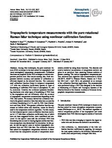
Figure 1: Brightness temperature as a function as of frequency in the of microwave spectrumin (V-Band: 50Fig. 1. Brightness temperature a function frequency the mi-
crowave (V-Band: 50–60 GHz). The spectrum (black line) 60 GHz). Thespectrum spectrum (black line) is calculated for the long-term average Payerne atmospheric state. is calculated for the long-term average Payerne atmospheric state. The colored, dashed vertical lines show the center frequencies of together with their band passes (normalized 1). the MWR HATPRO channelsto together with their band passes (normalized to 1). The colored, dashed vertical lines show the center frequencies of the MWR HATPRO channels
contain information on the vertical profile of temperature within the lower and middle troposphere due to the homogeneous mixing of O2 (Crewell and L¨ohnert, 2007). The receivers of each frequency band are designed as filter-banks in order to acquire each frequency channel in parallel. In addition, this approach allows setting each channel band pass individually. Typical HATPRO channel band passes are illustrated in Fig. 1. Unfortunately, the exact center frequencies and band passes for the instrument analysed in this study have not been determined yet. The band passes shown in Fig. 1 are from an identically constructed instrument operated by the University of Madison, WI, USA and are currently the best estimate available. A steerable parabolic mirror, covered by a microwave transparent radome, guarantees that radiation from ±90◦ elevation may be received at the radiometer. The radome is protected by a heated blower system to prevent the formation of dew and the accumulation of precipitation. The antenna beam width for the channels along the oxygen line is 2–2.5◦ full width at half maximum (FWHM) with a side lobe suppression of better than 30 dB so that 99.9 % of the received power stems from an angular range of ±3◦ . Additionally, falling precipitation is flagged by an automatic precipitation sensor and furthermore, environmental sensors for temperature, humidity and pressure as well as a GPS clock are part of the system. The measurement quantity of a MWR is brightness temperature (TB). Instead of calibrating in terms of radiance (W m−2 sr−1 Hz−1 ), where one would be dealing with very small numbers over a few degrees of magnitude, the DC radiometer output voltage is directly converted into a brightness temperature via the Planck function. This implies that Atmos. Meas. Tech., 5, 1121–1134, 2012
1124
U. L¨ohnert and O. Maier: Operational profiling of temperature using MWR
the range of measurements will be between 2.7 K (cosmic background) and ambient temperature. Absolute calibration for the channels of the V-band is performed using a liquid-nitrogen-cooled load that is attached externally to the radiometer box during maintenance. The cooled load can be considered as a black body at the LN2 boiling temperature of ∼77 K. This standard – together with an internal ambient black body load – is used for the absolute calibration procedure. Note that when looking at a perfect black body the physical temperature and the Planckequivalent brightness temperature are identical. Assuming a linear characteristic of the detector diode, these two points then lead to an absolute calibration of the MWR. During the time period from 2006 to 2009 five LN2 calibrations were performed at the dates listed in Table 1. Further details on the HATPRO calibration procedure, i.e. on the detector nonlinearity correction and the continuous gain adjustment are given by Rose et al. (2005). 3.2
Radiosonde
At Payerne a PTU (Pressure, Temperature, hUmidity) radiosonde is launched twice a day at 00:00 and 12:00 UTC. The radiosonde is launched one hour before the official time to cope with ascent times and data processing issues, however the exact launch time is coded within the sounding data. The radiosonde flies through the atmospheric Boundary Layer (BL) and reaches an elevation of approx. 3000 m within the first 10 min and reaches 10 km within approx. 30 min of flight. It then generally continues up to 30 km. After the first 20 s of flight, the time resolution of the samples varies from 1 s to 10 s, which gives a vertical resolution that ranges from 10 to a maximum of 80 m. The Swiss radiosonde SRS 400 used here was introduced in 1990. The sensors of this radiosonde include copperconstantan thermocouples of 0.063–0.050 mm diameter for temperature, a full range water hypsometer for pressure, and a carbon hygristor for relative humidity (Richner and H¨unerbein, 1999). The accuracies of the sensors are listed in Table 2. 3.3
Tower measurements
The 30 m BSRN-tower (Baseline Surface Radiation Network) is located 200 m to the south of the HATPRO site and radiosonde launch area. It has sensors for environmental measurements at 2, 10 and 30 m respectively. The temperature sensors have precisions better than 0.2 K throughout the whole dynamic range and deliver instant values every 10 min. The tower measurements were used as a comparison with the radiosonde to evaluate the differences between two in-situ methods, which can then be set into relation with the differences between radiosonde and MWR. At 30 m above ground, the BIAS between BSRN sensor and radiosonde and over the time period from 1993 to 2004 (7625 samples) is Atmos. Meas. Tech., 5, 1121–1134, 2012
Table 1. Absolute calibration times of the HATPRO instrument at Payerne between 2006 and 2009. Date
Time (UTC)
28 September 2006 24 April 2007 24 October 2007 28 March 2008 17 September 2009
12:00–13:00 13:00–14:00 07:00–08:00 13:00–15:00 12:00–14:00
0.07 K, whereas the standard deviation of the difference between BSRN and radiosonde is 0.53 K. Note that the differences include uncertainties due to the altitude of the radiosonde (±10 m according to the precision of the hypsometer) and due to linear interpolation in height, because the radiosonde rarely gives a value at exactly 30 m. 4
Data quality control
All radiosondes from 1992–2009 were quality controlled for physical consistency according to N¨orenberg et al. (2008). This resulted in 12 524 radiosondes that could be used for temperature retrieval development. During the time period of MWR measurements from August 2006–December 2009, a total of 2107 quality-controlled all-season, all-weather radiosondes could be matched in time to MWR measurements. This is far more than during previous studies, such as during the TUC experiment, which could only account for about 220 radiosondes. An MWR temperature retrieval was carried out every 12–13 min of which the closest in time was used for comparison against the radiosonde ascent. The study relies on ∼24 000 h of HATPRO measurements from August 2006 until December 2009. Most of the time the instrument operated continuously (average data availability >90 %), except for a longer period of maintenance from 11 May to 17 September 2009 following a 2 months period with intermittent failure. A number of quality checks, respectively correction procedures were applied to the MWR brightness temperatures to ensure that only trustworthy data flows into the analysis: – Cases where the MWR precipitation sensor detected rain (or snow) were excluded from the analysis. – Cases when the MWR recorded non-physical brightness temperatures (i.e. lower than 2.7 K or higher than a threshold value of 330 K) or retrieved non-physical air temperatures (i.e. lower than 180 K and higher than 330 K) were excluded from the analysis. – All the data were cross-checked “by eye” to exclude inconsistent spikes in the TB-channels, which may be caused by Radio Frequency Interference (RFI) or non-meteorological “disturbances” (sun, moon, humans, birds, aircraft, . . . ). www.atmos-meas-tech.net/5/1121/2012/
APRIL 2012 U. L¨ohnert and O. Maier: Operational profiling of temperature using MWR Table 2. Accuracies of the Swiss SRS400 radiosonde sensors. Sensor type
Temperature
copper-constantan thermocouples
±0.2 K
Pressure
water hypsometer
±2 hPa (accuracy increases with height)
Humidity
carbon hygristor until April 2009
±10 to 20 %
capacitive polymer starting May 2009
±5 to 10 %
MAIER
1125
Atmospheric profiles from radiosondes
Accuracy in the troposphere
Parameter
LÖHNERT AND
2006 - 2009
1992– 2009
T(z)
p(z), T(z), q(z), LWC(z) Radiative transfer model
TBs from radiometer 2006 - 2009
Calculated TBs
– Periods after strong precipitation where the dew blower was not powerful enough to evaporate the water on the radome immediately were also excluded “by eye” from the analysis.
615 These quality controls lead to a reduction of the total available MWR data for the radiosonde comparison of about 14 %, whereby 4 % were rejected due to cross-checking “by 616 eye”. The latter point still remains an open issue for all operational MWR applications: cross-checking “by eye” is cer617 tainly not an option for an operational MWR application, although necessary for the analysis of the current data set. 618 This clearly demands for sophisticated automatic RFI filters, as well as for quality controls concerning the sanity of the receiver system. 619 5 Temperature retrieval The retrieval algorithm (Fig. 2) uses simulated TBs at required frequencies and elevation angles (see below) derived from the 1992–2009 Payerne radiosonde data via radiative transfer calculations using pressure, temperature and humidity profiles of each sounding. Liquid clouds are assumed to be present at temperatures above −20 ◦ C and at relative humidity values higher than 95 %. The liquid water content is calculated with a modified liquid adiabatic model based on an empirical correction accounting for entrainment (Karstens et al., 1994). Temperature and pressure information was generally available up to 30 km height for the simulation, so that no systematic under-estimation is expected due to the omission of layers in the stratosphere, which contribute to the microwave signal. For the radiative transfer simulations, gaseous absorption is calculated according to Rosenkranz (1998), whereby the water vapor continuum is modified according to Turner et al. (2009) and the 22 GHz water vapor line width is modified according to Liljegren et al. (2005). The latter could show that the broadening of the line also has influence on the Vband channels. www.atmos-meas-tech.net/5/1121/2012/
Statistical multi-linear regression coefficients
Retrieval of profiles 2006 - 2009
comparison
Figure 2: chart Flowofchart of derivation retrieval and derivation andpercomparisons Fig. 2. Flow retrieval comparisons formed in this study. Note that the following input is needed in order tofollowing perform radiative calculations: temperature profile T (z), inputtransfer is needed in order to perform radiative transfer pressure profile p(z), humidity profile q(z), liquid water content profile LWC(z). pressure profile p(z), humidity profile q(z), liquid water content For retrieval derivation we have applied monochromatic simulations at the center frequencies of HATPRO (Fig. 1) assuming infinitively small antenna beam widths (pencil beam approximation) – both representing common approximations. The effects of these approximations are discussed in Sect. 5.2. 5.1
Theory
At the opaque center of the O2 absorption complex at 60 GHz, most of the temperature information originates from near the surface, whereas further away from the center, the atmosphere becomes less and less opaque so that more and more information also originates from higher atmospheric layers. Using the frequency dependent information alone at zenith results in the order of ∼2.5 independent pieces of vertical temperature information throughout the troposphere (L¨ohnert et al., 2009). Since the development of the BL is of special interest due to the large transfer of energy between the surface and the atmosphere, a higher vertical resolution, especially in the lower troposphere is desired. Therefore combined elevation scanning and multiple frequency methods have been developed by Crewell and L¨ohnert (2007). The retrieval presented here uses the same brightness temperature measurements at six elevation angles 90.0◦ , 42.0◦ , 30.0◦ , 19.2◦ , 10.2◦ and 5.4◦ Atmos. Meas. Tech., 5, 1121–1134, 2012
1126
U. L¨ohnert and O. Maier: Operational profiling of temperature using MWR
corresponding to air mass factors of about 1, 1.5, 2, 3, 5, and 10. By assuming horizontal homogeneity of the atmosphere, the observed radiation systematically originates from higher altitudes the higher the elevation angle. In case of an optically thick channel (i.e. when all of the radiation received at the radiometer originates from the closer environment of the instrument), the lower elevation angles can be attributed to the temperature in the lower layers, whereas higher elevation angles contain temperature information from multiple layers higher above. This fact leads to high accuracy temperature retrievals in the lowest 1 km and can enhance the number of independent pieces of vertical temperature information to ∼4. Since brightness temperatures of optically thick channels typically vary only slightly with elevation angle, elevation scanning temperature retrievals require highly sensitive radiometers, a fact which is realized in the HATPRO instrument by a high thermal stability and by using wide bandwidths up to 2 GHz in the optically thick channels 56.66– 58.00 GHz. In contrast, the lower four channels have bandwidths of 230 MHz in order to guarantee a higher degree of spectrally independent information. 5.2
Implementation
As performed by Crewell and L¨ohnert (2007), a multi-linear regression between the forward modelled TBs and atmospheric temperature as measured by the radiosonde at a defined height level is carried out. Temperature profiles are then retrieved from the TBs measured with the radiometer from 2006 to 2009, using the derived regression coefficients. Algorithms were developed up to a height of 10 km above ground level on a 50 m spacing vertical grid close to the ground gradually increasing to 1 km in the upper troposphere. Note that this grid is much finer than the true vertical resolution of the retrievals but similar to the one used by current weather forecast models. Elevation scans were performed every 12– 13 min, so that high-quality temperature profiles are available approximately four times an hour. In between, zenith observations are performed to infer atmospheric water vapor and liquid water path. Next to the random temperature errors, the retrievals are also almost always subject to systematic error. Such errors can originate from instrumental effects as well as from the radiative transfer simulation. In the following we show how systematic errors may be reduced through assessing the systematic TB offsets. We observe that during clear sky situations at Payerne, V-band HATPRO measurements and radiative transfer calculations using collocated radiosonde data show significant differences. For selecting sounding cases at clear sky conditions, the product APCADA (Duerr and Philipona, 2004) is used, that derives a global cloud coverage estimation from radiation measurements at Payerne, although it does not necessarily detect thin cirrus clouds, which is irrelevant here, because HATRPO measurements are insensitive to cirrus. Typically, APCADA values of 0 or Atmos. Meas. Tech., 5, 1121–1134, 2012
1 octa are considered as clear sky conditions. For the selected cases, the LWP values derived from the MWR are then cross checked one hour before and two hours after the radiosonde launch for being close to zero and stable. Principally we do not expect a perfect agreement because the MWR performs a point measurement in time and captures the whole atmospheric column within an instant, while the radiosonde is subject to wind drift and has an ascent time of ∼30 min before reaching the top of the troposphere. However, no significant systematic error is to be expected from this discrepancy. The results of these comparisons are shown in Fig. 3, which makes clear that large systematic offsets of up to 5 K and more are evident in the more transparent V-band channels. Note, that Hewison et al. (2006) also observed offsets on the same order of magnitude employing radiometers from a different manufactorer. TB offsets are also present in the off-zenith observing directions as shown in Table 3, where the necessity of considering the offset correction for the optically thinner frequency channels even down to low elevation angles becomes apparent. The temporal variation of the TB offsets (Table 3) is less than 0.5 K for the channels that are more optically thick. In contrast to this, the two optically thinner channels (51.26 and 52.28 GHz) show variations up to 2.5 K. Since these channels are more transparent, the effects of the time delay and the spatial drift of the radiosonde with respect to the instantaneous MWR measurement are more evident. Additionally, these variations arise from radiometric noise as well as from random uncertainties in the oxygen absorption model. The fact that some of the observed offsets seem to “jump” after each LN2 calibration, hints towards a problem with the calibration. Typical error sources in the LN2 calibration procedure are water condensate forming on the aluminium plate reflector connecting the cold load and the radiometer or on the radiometer radome itself, as well as a non-homogenous covering of the absorber material of the cold load with LN2 . TB offsets after the first, second and fourth calibrations resemble each other, while the TB offsets after the third and fifth calibration are also similar to each other. We here assume that the third and fifth calibrations were faulty in the sense that water condensate formed on the aluminium plate or the radome leading to an additional emission signal and in consequence to a underestimation of the TBs as shown in Fig. 3. In order to prevent this, MWR radome blowers and heaters should be operated with maximum power and continuous checks of the radome state should be carried out during calibration. Assuming that the first, second and fourth LN2 calibrations were performed correctly, the following possible sources remain to describe the TB offsets: Center-frequency offset: a systematic TB BIAS could results from the fact that the nominal center-frequency of a specific channel does not correspond to the actual center frequency the instrument is measuring at. In order to quantify this possible error, we have calculated the shift in www.atmos-meas-tech.net/5/1121/2012/
26
TB(MWR)-TB(radiosonde) [K]
TB(MWR)-TB(radiosonde) [K]
TB(MWR)-TB(radiosonde) [K]
APRILO.2012 AND M AIER U. L¨ohnert and Maier: Operational profilingLÖHNERT of temperature using MWR 51.26 GHz
52.28 GHz
5
5
0
0
-5
-5
-10
-10 01-Mar
01-Sep
01-Apr Date
01-Nov
01-Jun
01-Dec
01-Mar
01-Sep
53.86 GHz
01-Apr Date
01-Nov
01-Jun
01-Dec
01-Jun
01-Dec
01-Jun
01-Dec
54.94 GHz
5
5
0
0
-5
-5
-10
-10 01-Mar
01-Sep
01-Apr Date
01-Nov
01-Jun
01-Dec
01-Mar
01-Sep
56.66 GHz
01-Apr Date
01-Nov
58.00 GHz
5
5
0
0
-5
-5
-10
-10 01-Mar 2007
620
1127
01-Sep
01-Apr 2008
01-Nov
01-Jun
01-Dec
2009
01-Mar 2007
Date
01-Sep
01-Apr 2008
01-Nov 2009
Date
Fig. 3. TB offset time series at 90◦ elevation for 6 HATPRO V-band channels: TB(measured by MWR)-TB(simulated from sonde). The thick 621 Figure the 3: absolute TB offset time series 90°liquid elevation for 6 HATPRO V-band channels: TB(measured by vertical lines indicate calibration timesatwith nitrogen.
622
MWR)-TB(simulated from sonde). The thick vertical lines indicate the absolute calibration times with
Table 3. Clear sky offsets (MWR – simulated from sonde) and their 623deviations liquid(both nitrogen. standard in K) for the MWR elevation angles and optically thin V-band frequency channels during the period between the fourth 624 and fifth LN2 calibration (268 cases). Elevation angle/channel in GHz 90◦ 42◦ 30◦ 19.2◦ 10.2◦ 5.4◦
51.26
52.28
53.86
54.94
3.96/1.70 5.70/1.73 5.51/1.99 5.04/2.33 2.22/1.48 0.52/0.95
0.23/1.32 0.71/1.22 −0.01/1.26 −0.49/1.29 −0.89/0.62 −0.44/0.42
1.50/0.51 0.96/0.43 0.59/0.38 0.35/0.38 0.14/0.40 −0.10/0.41
−0.35/0.39 −0.03/0.47 −0.04/0.42 −0.08/0.44 −0.15/0.47 −0.20/0.46
mid-frequency necessary to match the observations to the simulations (Table 4). These calculations are based on the 1992–2009 mean atmospheric profiles of temperature, pressure and humidity of Payerne. Only monochromatic and infinitively narrow (pencil beam) radiative calculations have been considered. The highest shifts on the order of −140 to −80 MHz are necessary at the most transparent channel 51.26 GHz. At the other channels the necessary shifts are on the order of −30 to +20 MHz. Measurements of the exact center-frequencies from an identically constructed HATPRO www.atmos-meas-tech.net/5/1121/2012/
instrument have shown differences to the nominal frequencies on the order of −30 to +80 MHz, so that the incomplete knowledge on the exact mid-frequency may account for a large parts of the offset. However it must again be underlined, that no exact measurements of the mid-frequency are available for the instrument used here so that this is only a potential, while plausible error source. Note, in contrast to the older Generation 1 (G1) HATPRO type used in this study, the current Generation 2 (G2) of HATPRO exhibits exactly determined mid-frequencies with an accuracy of better than 1 MHz considering the complete receiver system response. RPG (T. Rose, personal communication, 2011) has compared multiple G2 instruments to a reference radiometer and found maximum TB differences of 0.5 K at the optically thin Vband channels. Band pass effect: Fig. 4 shows the effects of the consideration of HATPRO band passes given in Fig. 1. In order to calculate the band-pass-averaged TB, monochromatic radiative transfer calculations were carried at a total of 40–50 (depending on the channel) frequencies ranging from the minimum to the maximum of the bandpass and averaged accordingly. On average, the BIAS between bandpass-averaged and center-frequency monochromatic TB simulations is smaller than 0.4 K in the V-band, except at the 53.86 GHz channel, where the monochromatic approximation can lead to an
Atmos. Meas. Tech., 5, 1121–1134, 2012
LÖHNERT AND MAIER 27 using MWR U. L¨ohnert and O. Maier: Operational profiling of temperature
APRIL 2012
1128
TB (mc, pb) - TB (bdp, pb) [K]
0.5 0.0 -0.5 -1.0
TB (mc, pb) - TB (mc, bmw) [K]
50
52
54
Fre qu enc y [ GH z]
56
58
60
0.5 0.0 -0.5 -1.0 50
625
RMS-Difference
TB (mc, pb) - TB (mc, bmw) [K]
TB (mc, pb) - TB (bdp, pb) [K]
BIAS
52
54 56 Frequency [GHz]
58
60
0.14
Elev.: 90.0 Elev.: 42.0 Elev.: 30.0 Elev.: 19.2 Elev.: 10.2 Elev.: 5.4 N= 2579
0.12 0.10 0.08 0.06 0.04 0.02 0.00
50
52
5 4
Freq u enc y [GH z]
56
58
6 0
0.14 0.12 0.10 0.08 0.06 0.04 0.02 0.00 50
52
54 56 Frequency [GHz]
58
60
Fig. 4. Differences in simulated TBs: monochromatic (mc), infinitively narrow beam (pencil beam: pc) assumption minus realistic HATPRO 626 concerning Figure 4: in simulated TBs: monochromatic (mc),panels infinitively narrow beam (pencil beam: specifications theDifferences band pass (bdp) and beam width (bmw). The upper show the effects considering band pass characteristics, while the lower panels show the effects of actual beam width. Left: systematic differences, right: random differences. The calculations 627all-sky pc)radiosonde assumption minusand realistic HATPRO specifications concerning the bandpass (bdp) and beam rely on 2579 ascents are shown for different elevation angles (colored).
628
width (bmw). The upper panels show the effects considering band pass characteristics, while the lower
underestimation on the order 1 K at 90◦ elevation. ThisLeft: systematic higher than 54 GHz in the random temperature retrieval, we can ne629 panels show the of effects of actual beam width. differences, right: differences. high deviation can be explained by the width of the band glect the beam width effects from our current discussion. pass, which the absorption-line-peak at ∼53.6 GHz. ascentsGaseous absorption model:elevation studies angles comparing different 630 “sees” The calculations rely on 2579 all-sky radiosonde and are shown for different This effect, however, cannot explain the difference between oxygen absorption models for the microwave spectrum (e.g. 631 and (colored). measurement model – a consideration of this pheHewison et al., 2006 or Cadeddu et al., 2007) have shown nomenon leads to an even larger difference between measystematic offsets between model and measurement that are surement632 and model because of opposite signs. Note, that on the same order of magnitude as the differences shown the variability of the differences are rather small, i.e. behere. Thus, it is not possible in this study to discriminate below 0.1 K. It is important to note, that RPG has redesigned tween the possible sources of discrepancy. 633 (narrowed) the band passes of the first four HATPRO VRadiosonde: we do not expect the systematic differences band channels significantly for the G2 instruments leadto originate from the radiosonde measurements because these 634 ing to BIAS values between bandpass-averaged and centerwould imply unrealistically large temperature offsets (0.5 K) frequency monochromatic TB simulations lower the 0.2 K varying with height in the lower to middle troposphere. overall. 635 For each measurement period between two subsequent Beam width effect: radiative transfer calculations considLN2 calibrations, a separate offset correction procedure is 636 beam widths of 2.25◦ FWHM are compared ering realistic developed and applied to every TB measurement. This corto the mono-chromatic, pencil-beam calculations (Fig. 4). At rection is carried out via a linear relation depending on the 637 all frequencies and angles larger than 19.2◦ , the beam width measured TB itself and is also a function of frequency and effects are smaller than 0.15 K and thus mostly negligible in elevation angle. The TBs with and without the offset correccontrast 638 to other effects. However, at elevation angles lower tion are both applied to MWR measurements and the results than 19.2◦ and the lower two frequency channels, systemare discussed in Sect. 6 below. atic differences up to 0.7 K occur. These overestimations of the pencil beam approximation may be attributed to a higher 6 Data analysis degree of saturation in the lower part of the beam. Because lower elevation angles than 90◦ are used only at frequencies The following retrieval data analysis assesses the accuracies of MWR temperature retrievals under different conditions. Atmos. Meas. Tech., 5, 1121–1134, 2012
www.atmos-meas-tech.net/5/1121/2012/
U. L¨ohnert and O. Maier: Operational profiling of temperature using MWR
1129
Table 4. Necessary center frequency shifts [in MHz] to account for the systematic differences shown in Fig. 3.
51.26 GHz 52.28 GHz 53.86 GHz 54.94 GHz APRIL 2012
LÖHNERT AND
Before 1st calibration
After 1st calibration
After 2nd calibration
After 3rd calibration
After 4th calibration
After 5th calibration
−170 −10 +10 +90
−140 ±0 −20 +40
−80 +20 −20 +40
+190 +160 +30 +180
−140 −10 −30 +20
+100 +80 ±0 +180
APRIL 2012
28
MAIER
Temperature 4
294
LÖHNERT AND
29
MAIER
4
4
3
3
288 282 277
3
265
Kelvin
Height [km]
260
2
Height [km]
Height [km]
271
2
2
1 1
1
0 0
639
6
12 Hours on 20080908 [UTC]
18
24 0 265
640
Figure time-heighttime-height temperature contours between 0 and 4contours km on 09 September, Fig. 5:5.MWR-retrieved MWR-retrieved temperature between649
641
0 and 2008.
4 km on 9 September 2008.
642 643 644 645 646 647 648
275 280 285 Temperature 0 UTC [K]
290
0 265
270
275 280 285 290 Temperature 12 UTC [K]
295
650
Figure profile atprofile 0 (left) andat 12 00:00 (right) UTC on 09 and September 2008 (right) between 0 and 4 Fig. 6:6.Temperature Temperature (left) 12:00 UTC
651
onThe 9 September 2008 between km. shows the km. bold line shows the radiosonde profile, 0 theand dotted4line the The MWR bold retrievalline and the dashed line
652
radiosonde profile, thewith dotted line the MWR the radiosonde profile smoothed the averaging kernel.
We have chosen to divide the analysis into cases only dur-653 ing clear-sky and then for all-sky conditions. Additionally we look into the differences of retrieval performance during day and night and try to identify the reliability of MWR temperature retrievals during significant weather, i.e. frontalpassages and cold/warm extremes As an example of a continuous MWR temperature profile retrieval over 24 h, Fig. 5 shows a time-height contour of a late summer day with a typical development of the BL starting from a night-time inversion towards a well mixed daytime BL. After sunset, IR cooling induces again an inversion close to the surface. A warming of ∼4 K in the altitude range between 2 and 4 km can also be observed throughout the course of the day. Both at 00:00 and 12:00 UTC the MWR retrieval is able to accurately reproduce the radiosonde profile in the region below 1 km (Fig. 6). Especially the low-level inversion at night is nicely captured. Above 1 km, the limited vertical resolution of the MWR measurements become obvious, i.e. during both cases the lifted inversions are not retrieved. Using the average (1992–2009) Payerne profile of temperature, humidity and pressure, the number of independent pieces of information contained in the TB for retrieving the temperature profile (degrees of freedom for signal, DOF) can be determined following Rodgers (2000). The calculated averaging kernels for 6 distinct heights are shown www.atmos-meas-tech.net/5/1121/2012/
270
retrieval and the dashed line the radiosonde profile smoothed with the averaging kernel.
in Fig. 7, which are defined by the sensitivity of the retrieved value at height with index i to the true value at height j (δTretrieved,i /δTtrue,j ). Note, a perfect vertical resolution would give rise to a delta function with a value of 1 at height i = j and 0 at all other heights i 6= j . Thus, the broadness of the averaging kernels gives information on the vertical resolution. The diagonal components of the averaging kernel matrix A correspond to the DOF for each level and the trace of the averaging kernel matrix yields the total DOF, which are ∼4 in case of the temperature retrieval. If the cumulative distribution of the DOF with height is regarded (Fig. 7), one can conclude that about 85 % (95 %) of the temperature information originates from the lowest 2 km (4 km). The radiosonde profile can be brought onto the vertical resolution of the MWR temperature retrieval by the following multiplication (averaging kernel smoothing): T smoothed = T retrieved + A (T true − T retrieved )
(1)
This accounts for the limited vertical resolution of the MWR temperature retrieval and the resulting differences can now be analysed more precisely towards measurement, forward modelling or statistical representativeness error. In Fig. 6, the smoothed radiosonde profile is very close to the MWR Atmos. Meas. Tech., 5, 1121–1134, 2012
1130
APRIL 2012
LÖHNERT AND
MAIER
U. L¨ohnert and O. Maier: Operational profiling of temperature using MWR 30
APRIL 2012
LÖHNERT AND
31
MAIER
4
Height [km]
3
2
STDEV OC, AVK
1
BIAS OC, AVK STDEV OC
654
BIAS OC
655 656 657 658 659 660
Fig. Temperature kernels /δTprofile ) for Figure 7. 7: Temperature averagingaveraging kernels (δTretrieved,i /δTtrue,j) for(δT the mean temperature the true,jfrom retrieved,i the mean temperature profile from the complete Payerne data set complete Payerne data set (1992-2009) as a function of height shown for different heights of (1992–2009) as a function of height shown for different heights of perturbation (left). Cumulative Degrees of Freedom (DOF) for temperature with height (right). The perturbation (left). Cumulative Degrees of Freedom (DOF) for tem- 661 DOF at eachwith height height corresponds to the diagonal value of averaging kernel. The four different perature (right). The DOF attheeach height corresponds to 662 curves correspond to different seasons (summer/winter) and different radiosonde ascent (0/12 the diagonal value of the averaging kernel. The four differenttimes curves 663 correspond different (summer/winter) and different raUTC) derived fromtocomplete Payerneseasons data set (1992-2009). 664 diosonde ascent times (00:00/12:00 UTC) derived from complete 665 Payerne data set (1992–2009). 666 667
retrieval in the lowest 2 km, however it becomes clear that 668 the MWR retrieval cannot resolve the exact details shown within the radiosonde profile, i.e. the night-time isothermal layer from 1 to 1.3 km. During night above 2 km, a persistent underestimation (1–2 K) of the MWR retrieval occurs between radiosonde and retrieved profile as well between smoothed and retrieved profile. This points to the fact, that this underestimation is not due to vertical resolution effects but is more likely due to one of the error sources mentioned above. 6.1
Clear sky comparisons
In order to test the consistency of the TB offset correction procedure, a first clear-sky comparison is carried out. Here, the temperature retrieval coefficients are derived using exactly the same 487 clear-sky cases as for deriving the TBoffset corrections (Sect. 5.2). This retrieval was then again applied to the corresponding clear-sky MWR measurements: once applying the TB offset correction and once using the original TBs (Fig. 8). If the TB offset correction is not applied, systematic differences between −0.7 and +0.2 K arise in the lowest 4 km. The systematic difference is even similar in size to the random difference in the boundary layer. As expected, a clear positive influence of the TB-offset correction can be seen both with respect to BIAS as well as STDEV between MWR and radiosonde temperature. The BIAS has practically vanished throughout the profile and the STDEV values range within 0.4 and 1.3 K within the lowest 2 km increasing to 1.5 K at 4 km. The overall lowest STDEV can be observed at 250 m with a value of ∼0.4 K. The STDEV value decreases from 0.75 K at the surface to this value due to the high temperature variability directly close to the surface Atmos. Meas. Tech., 5, 1121–1134, 2012
STDEV BIAS
0 -0.5
0.0
0.5 1.0 Temperature difference [K] MWR - Sonde
1.5
2.0
2.5
Figure 8. 8: Temperature Temperature profile differences (BIAS and STDEV) during conditions from Fig. profile differences (BIAS andclear-sky STDEV) during clear-sky between August 2006 –conditions December 2009 from betweenAugust MWR and 2006–December radiosonde measurements.2009 The MWR retrieval MWR and radiosonde measurements. The MWR retrieval coefficoefficients and the TB-offset correction were derived using exactly the same clear-sky measurements cients and the TB-offset correction were derived using exactly the as considered in the evaluation. Black lines show the retrieval results without using the systematic TB same clear-sky measurements as considered in the evaluation. Black offset correction whileretrieval green lines show the results applyingusing the systematic TB offset correction lines show the results without the systematic TB (OC). offset correction while show the results profile applying sysAdditionally, in red the STDEVgreen is shownlines after smoothing the radiosonde with thethe averaging tematic TB offset correction (OC). Additionally, in red the STDEV kernel (AVK). A total number of 486 matching MWR/radiosonde cases are evaluated in the plot. is shown after smoothing the radiosonde profile with the averaging kernel (AVK). A total number of 486 matching MWR/radiosonde cases are evaluated in the plot.
coupled with the fact that MWR is sensitive to a volume of air, whereas the radiosonde measures at relatively fixed points in time and space. Additionally the radiosonde needs typically 50 m to reach an equilibrium temperature concerning its natural ventilation due to ascent speed. Additionally, Fig. 8 shows the BIAS and STDEV values using the smoothed radiosonde profiles (Eq. 1). Whereas the BIAS using the smoothed and non-smoothed radiosonde values do not differ, the STDEV values are much lower and range from 0.3 to 0.7 K in the lowest 4 km. These numbers are the errors to expect from the random uncertainty in TB measurement (0.2–0.5 K) as well as from the radiosonde measurement. Hereby, the latter is due not only to the sensor uncertainty of 0.2 K (Table 2), but also due to temporal delay and spatial drifts of the radiosonde with respect to the quasi-instantaneous MWR measurement. 6.2
All sky comparisons
Next, the retrieval performance is evaluated using 1816 simultaneous radiosonde/MWR measurements during all-sky conditions. Additionally to the clear-sky cases, this data set also contains cloudy cases. The retrieval algorithm coefficients, which are applied to this data set, are derived from all 1992–2009 radiosondes as seen in Fig. 2 and described in Sect. 5. Using 12 524 radiosondes from this time span allows to develop a much more robust algorithm that is applicable www.atmos-meas-tech.net/5/1121/2012/
APRIL 2012
LÖHNERT AND
33
MAIER
U. L¨ohnert and O. Maier: Operational profiling of temperature using MWR LÖHNERT AND MAIER 32 683
1131
APRIL 2012
4
Height [km]
3
2
STDEV OC, AVK
1
BIAS OC, AVK STDEV OC BIAS OC STDEV BIAS
0 -0.5
669
0.0
0.5 1.0 Temperature difference [K] MWR - Sonde
1.5
2.0
2.5
670
Figure profile differences and STDEV)(BIAS during all-sky from durAugust Fig. 9:9.Temperature Temperature profile (BIAS differences andconditions STDEV)
671
ing all-sky conditions from August 2006–December between 2006 – December 2009 between MWR and radiosonde measurements. 2009 The MWR retrieval
672
coefficients were derived from the whole 1992-2009 radiosonde data set, whereas and the TB
673 674 675 676 677 678 679 680 681 682
MWR and radiosonde measurements. The MWR retrieval coefficients were derived from the whole 1992–2009 radiosonde data set, correction was derived only from clear-sky measurements as in Fig. 8. Black lines show the retrieval whereas and the TB correction was derived only from clear-sky results without using the correction while green lines the results applying measurements assystematic in Fig.TB8.offset Black lines show the show retrieval results without using the systematic TB offset correction while green lines the systematic TB offset correction (BC). Additionally, in red the STDEV is shown after smoothing show the results applying the systematic TB offset correction (OC). the radiosonde profile with the averaging kernel (AVK). A total number of 684 2107 matching Additionally, in red the STDEV is shown after smoothing the raMWR/radiosonde cases were considered; in 1816 cases the MWR measurements passed the quality Fig. 10. Temperature error covariances calculated from all-sky condiosonde profile with the averaging kernel (AVK). A total 685number Figure 10: Temperature error covariances calculated from all-sky conditions from August 2006 – control and are evaluated in MWR/radiosonde the plot. ditions from August 2006–December 2009 between MWR and raof 1816 matching cases are evaluated in the plot. 686 Decemberdiosonde 2009 between MWR and radiosonde measurements. covariances measurements. The error covariancesThe areerror shown for six are shown for specific height levels. Asterisks show the reference heights. 687
six specific height levels. Asterisks show the reference heights.
for all cases between August 2006 and December 2009. Similar to the clear-sky comparison, systematic differences 688 range between −0.6 and +0.3 K in the lowest 4 km if the TB offset correction is not applied (Fig. 9). After applying the689correction the overall BIAS is smaller than ±0.1 K, except for the 690 offset surface point (+0.2 K). This makes clear that the TB correction derived from the clear-sky cases can also significantly help reducing the BIAS for all sky cases. Note691 that the STDEV values are very similar to the clear-sky values shown 692 in (Sect. 6.1, Fig. 8) underlining the potential of MWR for temperature profiling also during cloudy situations. For the TB-offset corrected values, the RMS values are within 0.4 to 1.4 K in the lowest 2 km and increase to 1.7 K at 4 km. The high accuracies below 1 km are primarily due to the information contained in the elevation scans (L¨ohnert et al., 2009). These long-term comparisons are also consistent with the predicted accuracies based on simulations by Crewell and L¨ohnert (2007) using an identical retrieval algorithm setup. Note, that BIAS and STDEV values using the smoothed radiosonde profiles in Fig. 9 are very similar to the clear sky values (Fig. 8) and range from 0.3 to 0.8 K in the lowest 4 km.
www.atmos-meas-tech.net/5/1121/2012/
In order to assess the retrieval uncertainty in a complete way, it is also necessary to calculate the level-to-level error covariances. These give information on the correlation of the temperature error in height i with the temperature error in height j as shown in Fig. 10 for six distinct heights. The relatively sharp and low maximum peak values below 1 km underline the high potential for BL temperature profiling, whereas increasing broadness and maximum peak values of the error covariance curves at heights above 2 km again underline decreasing vertical resolution and accuracy with increasing height. Such error covariance information is necessary for assimilating MWR temperature data into NWP models, i.e. within a 3DVAR or 4DVAR assimilation system. In order to correctly interpret Figs. 8 and 9, it is important to consider the availability of quality controlled MWR temperature data during the all-sky cases analysed. Within the period from August 2006 to December 2009, 2107 cases of simultaneous MWR and radiosonde measurements have been identified. 291 (∼14 %) of these cases are not included in the analysis of Fig. 9 because these did not pass the MWR measurement quality control due to reasons described in Sect. 4. In summary the Payerne MWR was able to deliver reliable and accurate temperature profiles in 86 % of all-sky cases, with an uncertainty ranging from 0.5 K in the lower boundary layer and rising up to 1.7 K at 4 km height. Atmos. Meas. Tech., 5, 1121–1134, 2012
1132 APRIL 2012
LÖHNERT AND
U. L¨ohnert and O. AMaier: Operational profiling of temperature using MWR PRIL 2012 LÖHNERT AND MAIER 35 34
MAIER
4
4
STDEV all STDEV front STDEV cold STDEV warm
3
Height [km]
Height [km]
3
2
STDEV inversion
2
1
1 BIAS day, Ts BIAS day BIAS night, Ts BIAS night
0 -0.2
693 694 695 696 697 698 699 700
-0.1
0.0
0.1 0.2 Temperature difference [K] MWR - Sonde
0.3
705
0.5
1.0 1.5 Temperature difference [K] MWR - Sonde
2.0
2.5
Figure profile differences during (STDEV) all-sky (1816), during frontal (252), warm Fig. 12: 12.Temperature Temperature profile (STDEV) differences all-sky
(1816), frontal (252), extreme (330), cold extreme (330), cold extreme (332)warm and temperature inversion (165) casesextreme (see text for(332) details) and from temperature inversion (165) cases (see text for details) from August 2006–December 2009 between radiosonde and MWR measurements.
August 2006 – December 2009 between radiosonde and MWR measurements.
6.4
Frontal and extreme conditions
712
6.3
Day vs. night effects
713 714
703 704
0 0.0
0.5
Figure11. 11: Temperature Temperature profileprofile differencesdifferences (BIAS) during (BIAS) all-sky conditions fromall-sky August 2006 –706 Fig. during conditions August 2009differentiated betweenbyMWR December from 2009 between MWR2006–December and radiosonde measurements day and and night; rared707 diosonde measurements differentiated by day and night; red lines lines show the retrieval results only at 12 UTC, whereas black lines only at 0 UTC. 920 12 UTC,708 show the retrieval results only at 12:00 UTC, whereas black lines respectively 896 0 UTC MWR measurements passed the quality control and are evaluated in the plot. only at 00:00 UTC. 920 12:00 UTC, respectively 896 00:00 UTC709 Dashed lines show retrieval results using 2m-temperature (Ts) as an additional predictor in the linear MWR measurements passed the quality control and are evaluated in 710 regression. the plot. Dashed lines show retrieval results using 2 m-temperature (Ts) as an additional predictor in the linear regression. 711
701 702
0.4
When analyzing TB offset corrected temperature retrievals715 for 00:00 and 12:00 UTC radiosondes separately, the STDEV 716 values are within 0.15 K of each other throughout the lowest 4 km. However, the BIAS shows a non-zero behavior as a717 function of height with opposite sign (Fig. 11). This behavior varies between −0.16 and +0.3 K at the surface and shows minima of ±0 K at 250, respectively 1300 m. This effect is due to the fact that the retrieval coefficients have been derived without discriminating between day and night. Systematic temperature offsets very similar in size and vertical structure are obtained when applying the retrieval exactly to those simulated TBs from the 1992–2009 data set from which the regression coefficients are derived. However, when differentiating again by day and night, the magnitude and height of the minimum/maximum bias depends strongly on the random TB uncertainty chosen when deriving the linear regression coefficients. As only radiosonde ascents at 00:00 and 12:00 UTC are available, BIAS errors will always be an issue, even if one would derive separate retrieval coefficients for day and night. A way to partially reduce these effects is to include 2 m temperature observations (Fig. 11). Instead of using only calculated TBs as predictors for the temperature profile in the multi-linear regression, the 2 m temperature is additionally included and the BIAS values are much lower at the surface. The positive amplitude of the BIAS values with height is also slightly reduced to 0.2 K throughout the lowest 4 km. Atmos. Meas. Tech., 5, 1121–1134, 2012
The so far shown results are valid for an average over all cases. However, it is also necessary to show how the MWR temperature retrieval performs in frontal or extreme atmospheric conditions, where it is especially important for models to receive accurate measurement input. The following subsets of cases are extracted from the radiosonde data set: Tables frontal conditions, warm extremes, cold extremes and extreme temperature inversions. A situation is classified as frontal when available records report a front or occlusion crossing Z¨urich (170 km NE of Payerne) up to 12 h before or after the launch of a Payerne radiosonde. The warm extremes are classified as cases when the surface temperature is outside of the 1-sigma range as a positive deviation, whereas cold extremes are classified as cases when the surface temperature is outside the 1sigma range as a negative deviation. If the radiosonde profile shows a continuous temperature rise with height below 4 km throughout a 500 m height interval, the profile is classified as an extreme temperature inversion case. As can be seen in Fig. 12 the STDEV can vary quite considerably with height depending on the subset of cases evaluated. Throughout the lowest 4 km the STDEV during frontal passages are even up to 0.5 K smaller than in the all-sky cases. This is due to missing inversions during frontal passages, in contrast to fair weather situations, i.e. during winter anti-cyclonic situations or when residual layers occur at night after a sunny day. This becomes clear when comparing to other extreme cases. In the 165 evaluated extreme inversion cases MWR temperature retrieval STDEV is smaller than 1 K below 400 m but is then larger than 2 K already at 2 km. www.atmos-meas-tech.net/5/1121/2012/
U. L¨ohnert and O. Maier: Operational profiling of temperature using MWR Inversions are detected, however their amplitude and sharpness are smoothed out, leading to large differences when comparing level-to-level with the vertically highly resolved soundings. The STDEV for the cold curve resembles the inversion curve because 45 % of the analysed inversion cases are also classified cold extremes (i.e. night-time inversion due to strong radiative cooling in winter). Warm extremes, which can be associated with well-mixed boundary layers, show up to 0.5 K better STDEV than the all-sky cases. For these cases, only less than 1 % are also classified as an inversion. Similarly, only less than 5 % of the frontal cases are classified as an extreme inversion event. This makes clear that the performance of the MWR temperature retrieval can be considered as reliable during frontal conditions. However, quality-controlled data availability decreases down to 60 % in these cases, which is a result of the activated internal HATPRO precipitation flag. Hence, temperature profiles during frontal passages can only be characterized well at times when precipitation is not reaching the surface and thus obscuring the MWR measurement. During all of the subsets analysed above, the BIAS between MWR and radiosonde varies between −0.5 and +0.5 K as a function of height.
7
Summary and conclusions
This study shows the current strengths and weaknesses of microwave radiometry for atmospheric temperature profiling using a unique set of collocated MWR and radiosonde measurements. While the advantages of high temporal resolution and un-manned routine observations must be stressed, a limited vertical resolution (with respect to radiosondes) and corresponding random error inherent within the measurement principle must be kept in mind. Random errors range on the order of 0.5 K in the lower boundary layer and rising up to 1.7 K at 4 km height. Above this height only 5 % independent information originates from the radiometer measurement itself. While MWR measurement may prove very valuable for NWP model applications considering the random error, this study has also quantified and corrected for systematic error. The different possible sources of the observed systematic differences are difficult to allocate in retrospective, but these are currently subject of intense study in the microwave remote sensing community (University of Cologne, NOAA-Severe Storm Laboratory, RPG). This study makes clear that future operational MWR measurements need to be monitored permanently during clear sky conditions, i.e. using simple nonscattering radiative transfer modelling. Such monitoring is necessary to identify possible TB-offsets. TB offset corrections are essential for providing an optimized temperature profile product. The observed “stability” (w.r.t. the radiosondes) between two LN2 calibrations makes clear that HATPRO type MWRs may only need LN2 calibrations on the time scale of one year or even less often. www.atmos-meas-tech.net/5/1121/2012/
1133
The quality control procedures and offset correction method described in this paper are currently subject of intense discussion within the newly-found “International network of ground-based microwave radiometers” (MWRnet; http://cetemps.aquila.infn.it/mwrnet/). It is currently a central platform for uniting European-wide MWR measurements under the aspect of harmonization of measurement modes, data formats, retrievals etc. and is embedded with the COST action ES0702 EG-CLIMET (European GroundBased Observations of Essential Variables for Climate and Operational Meteorology; http://www.eg-climet.org). Basics on MWR operations and advice for MWR users are given through this portal via an open WIKI site. Acknowledgements. The authors would like to thank the Meteo Swiss staff for their support of this work: Pierre Huguenin for installing and operating the HATPRO microwave radiometer at Payerne as part of the CN-MET project from 2006 to 2009, Pierre Jeannet, Gonzague Romanens, Gilbert Levrat and Roger Bersier for sharing their know-how on sounding practice and related science and Dominique Ruffieux, Bertrand Calpini and their teams, for their leadership in making advanced remote sensing techniques operational for meteorologists and modellers. We also thank Radiometer Physics GmbH (Thomas Rose) for providing instrument details leading to the insights gained in this study. We are also grateful to David D. Turner (formerly University of Wisconsin, Madison, Madison, USA, now NOAA Severe Storms Laboratory, Norman, Oklahoma, USA) for providing us with the HATPRO bandpass data and enlightening discussion. This work has been embedded in and partially sponsored by the European COST action ES0702 (EG-CLIMET) under the lead of Anthony Illingworth, who is driving the development of ground-based remote sensing networks for operational weather observation and forecasting. The Institute of Geophysics and Meteorology, research group Integrated Remote Sensing (Susanne Crewell) at the University of K¨oln has provided fruitful discussions as well as computing environment and evaluation tools for the success of this study. Edited by: C. von Savigny
References Cadeddu, M. P., Payne, V. H., Clough, S. A., Cady-Pereira, K., and Liljegren, J. C.: Effect of the Oxygen Line-Parameter Modeling on Temperature and Humidity Retrievals From Ground-Based Microwave Radiometers, IEEE T. Geosci. Remote, 45, 2216– 2222, 2007. Calpini, B., Ruffieux, D., Bettems, J.-M., Hug, C., Huguenin, P., Isaak, H.-P., Kaufmann, P., Maier, O., and Steiner, P.: Groundbased remote sensing profiling and numerical weather prediction model to manage nuclear power plants meteorological surveillance in Switzerland, Atmos. Meas. Tech., 4, 1617–1625, doi:10.5194/amt-4-1617-2011, 2011. Cimini, D., Hewison, T. J., Martin, L., G¨u ldner, J., Gaffard, C., and Marzano, F. S.: Temperature and humidity profile retrievals from groundbased microwave radiometers during TUC, Meteorol. Z., 15, 45–56, 2006.
Atmos. Meas. Tech., 5, 1121–1134, 2012
1134
U. L¨ohnert and O. Maier: Operational profiling of temperature using MWR
Crewell, S. and L¨ohnert, U.: Accuracy of boundary layer temperature profiles retrieved with multi-frequency, multi-angle microwave radiometry, IEEE T. Geosci. Remote, 45, 2195–2201, doi:10.1109/TGRS.2006.888434, 2007. Duerr, B. and Philipona, R.: Automatic cloud amount detection by surface longwave downward radiation measurements, J. Geophys. Res., 109, D05201, doi:10.1029/2003JD004182, 2004. G¨uldner, J. and Sp¨ankuch, D.: Remote Sensing of the Thermodynamic State of the Atmospheric Boundary Layer by GroundBased Microwave Radiometry, J. Atmos. Ocean. Tech., 18, 925– 933, 2001. Hewison, T. J., Cimini, D., Martin, L., Gaffard, C., and Nash, J.: Validating clear air absorption models using ground-based microwave radiometers and vice-versa, Meteorol. Z., 15, 27–36, 2011, 2006. Karstens, U., Simmer, C., and Ruprecht, E.: Remote sensing of cloud liquid water, Meteorol. Atmos. Phys., 54, 157–171, 1994. Lilgegren, J. C., Boukabara, S. A., Cady-Pereira, K., and Clough, S. A.: The Effect of the Half-Width of the 22-GhzWater Vapor Line on Retrievals of Temperature and Water Vapor Profiles with a Twelve-channel Microwave Radiometer, IEEE T. Geosci. Remote, 43, 1102–1108, 2005. L¨ohnert, U. and Crewell, S.: Accuraccy of cloud liquid water path from ground-based microwave radiometry. Part I. Dependency on Cloud model statistics, Radio Sci., 38, 8041, doi:10.1029/2002RS002654, 2003. L¨ohnert, U., Turner, D., and Crewell, S.: Ground-based temperature and humidity profiling using spectral infrared and microwave observations: Part 1. Simulated retrieval performance in clear sky conditions, J. Appl. Meteorol., 48, 1017–1032, doi:10.1175/2008JAMC2060.1, 2009.
Atmos. Meas. Tech., 5, 1121–1134, 2012
N¨orenberg, D., Crewell, S., L¨ohnert, U., and Rose, T.: Development of Ground Equipment for Atmospheric Propagation Conditions Assessment from 10 up to 90 GHz Frequency Bands (ATPROP) – ESA CONTRACT 19839/06/NL/GLC, Final Report, available through Institute for Geophysics and Meteorology, University of Cologne, Germany, 2008. Richner, H. and v. H¨unerbein, S.: Grundlagen aerologischer Messungen speziell mittels der Schweizer Sonde SRS 400, Ver¨offentlichungen der SMA-MeteoSchweiz Nr. 61, ISSN 1422-1381, available at: www.meteoswiss.ch (last access: 21 May 2012), 1999. Rodgers, C. D.: Inverse methods for atmospheric sounding: Theory and practice, World Scientific, 238 pp., 2000. Rose, T., Crewell, S., L¨ohnert, U., and Simmer, C.: A network suitable microwave radiometer for operational monitoring of the cloudy atmosphere, Atmos. Res., Special issue: CLIWA-NET: Observation and modelling of liquid water clouds, 75, 183–200, doi:10.1016/j.atmosres.2004.12.005, 2005. Rosenkranz, P.: Water vapor continuum absorption: A comparison of measurements and models, Radio Sci., 33, 919–928, 1998. Ruffieux, D., Nash, J., Jeannet, P., and Agnew, J. L.: The COST 720 temperature, humidity, and cloud profiling campaign: TUC, Meteorol. Z. , 15, 5–10, 2006 Turner, D., Caddedu, M. P., L¨ohnert, U., Crewell, S., and Vogelmann, A. M.: Modifications to the water vapor continuum in the Microwave suggested by ground-based 150 GHz Observations, IEEE T. Geosci. Remote, 47, 3326–3337, doi:10.1109/TGRS.2009.2022262, 2009.
www.atmos-meas-tech.net/5/1121/2012/