Operational Semantics of Hybrid Systems - Semantic Scholar

invited paper in Proc. of Hybrid Systems: Computation and Control (HSCC) LNCS 3414, Zurich, Switzerland, March 9-11, 2005

Operational Semantics of Hybrid Systems Edward A. Lee and Haiyang Zheng? Center for Hybrid and Embedded Software Systems (CHESS) University of California, Berkeley, 94720, USA [email protected], [email protected]

Abstract. This paper discusses an interpretation of hybrid systems as executable models. A specification of a hybrid system for this purpose can be viewed as a program in a domain-specific programming language. We describe the semantics of HyVisual, which is such a domain-specific programming language. The semantic properties of such a language affect our ability to understand, execute, and analyze a model. We discuss several semantic issues that come in defining such a programming language, such as the interpretation of discontinuities in continuous-time signals, and the interpretation of discrete-event signals in hybrid systems, and the consequences of numerical ODE solver techniques. We describe the solution in HyVisual by giving its operational semantics.

1

Introduction

Hybrid systems are heterogeneous systems that include continuous-time subsystems interacting with discrete events. They are effective models for physical systems interacting with software or undergoing discrete mode changes. Typically, the continuous subsystem is modeled by differential equations, while the discrete events are modeled by finite state machines. Transitions between states represent either discrete mode changes or actions taken by software subsystems. Most of the major contributions in hybrid systems have been in the construction of a systems theory, theories of control, and analysis and verification tools (see for example [1,2,3,4,5,6]). A few software tools have been built to support such analytical methods, such as Charon [7], CheckMate [8], d/dt [9], HyTech [10], Kronos [11], Uppaal [12], and a toolkit for level-set methods [13]. In addition, some software tools provide simulation of hybrid systems, including Charon [7], Hysdel [14], HyVisual [15], Modelica [16], Scicos [17], Shift [18], and Simulink/Stateflow (from The MathWorks). An excellent analysis and comparison of these tools is given by Carloni, et al. [19]. In this paper, we focus on the simulation tools, but take the perspective that hybrid systems are not so much “simulated” as “executed.” We view the ?

This paper describes work that is part of the Ptolemy project, which is supported by the National Science Foundation (NSF award number CCR-00225610), and Chess (the Center for Hybrid and Embedded Software Systems), which receives support from NSF and the following companies: Infineon, Hewlett-Packard, Honeywell, General Motors, and Toyota.

semantics of hybrid systems as a concurrent model of computation, and the “simulation” tools as compilers and/or interpreters for programming languages that happen to have a hybrid systems semantics. Although many of the issues are closely related to those that arise in the design of simulators (see for example [20]), the emphasis becomes one of modularity and predictable and understandable behavior, rather than one of accurate approximation of unachievable behavior. Of the above tools, Shift and Modelica probably come closest to reflecting this philosophy, since they are consistently presented as programming languages more than as simulation tools. The view of hybrid systems as executable computational artifacts was stimulated by the DARPA MoBIES project (model-based integration of embedded software), which undertook the challenging task of establishing an interchange format for hybrid systems. The goal was to facilitate exchange of models and techniques between tools. The effort was led by the key proponents of modelintegrated computing [21], the developers of Charon, CheckMate, and HyVisual, and users of Simulink/Stateflow. The result of this work was a formalism called HSIF (hybrid system interchange format) [22]. A proposal for the next generation of interchange format can be found in [19]. One of the key objectives of HSIF, that of model exchange among diverse tools, was at odds with another of its key objectives, that of defining an executable and complete hybrid systems semantics. The diverse tools represented by the HSIF community have significant differences in their semantics, often reflecting their differing objectives (e.g. verification vs. simulation). In this paper, we set aside the concern for interchange of models, and focus instead on defining a clean and complete hybrid systems semantics. The objective is to define behaviors, including subtle corner cases, by giving a complete semantics for a programming language. We have implemented the semantics in HyVisual [15] in a version scheduled to be released (in open-source form, as usual) concurrently with the publication of this paper.

2

Example Model

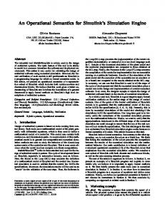
We start by considering a fairly typical hybrid system example shown in figure 1 that we can use to frame the discussion. The model is deliberately small and simple, making it easier to discuss semantic issues without the distracting complexity of a more “real-world” example. The figure shows the visual syntax of HyVisual [15], which is implemented within the Ptolemy II software framework [23]. The reader should not be misled by the visual syntax. While visual syntaxes are commonly used for models that approximate real systems, they can also be used as a programming language syntax, in which case the model is the real system (the program), in the same sense that the text of a C program is the program. We nonetheless call a visual program like that in figure 1 a “model” because calling it a “program” would confuse too many readers who assume that programs must have textual syntaxes. 2

Fig. 1. A hybrid system of two masses on springs.

The model in figure 1 is of a physical system consisting of two masses on springs that oscillate.1 When the masses collide, they stick together with an exponentially decaying stickiness. When the differential force of the springs exceeds the stickiness, the masses come apart. The three-dimensional rendition of the physical system shown in the figure is a snapshot of an animation created using the Ptolemy II graphics infrastructure [26]. The top-level of the hierarchy in the figure shows a continuous-time model, where boxes represent actors and connections between them represent continuous-time signals. The Masses block encapsulates the spring-masses model. The other three blocks are plotters. The next level of the hierarchy shows a finite-state machine with an (unimportant) initial state and two states representing the two modes of operation. Since states of this state machine represent modes of operation, we use the terms “state” and “mode” interchangeably for them. In the “Separate” mode, the masses are separately oscillating, and in the “Together” mode, they are stuck 1

This model was studied by Liu [24] and was inspired by microelectromechanical accelerometers [25].

3

together. The behavior in each of these modes is specified at the third level of the hierarchy shown in figure 2. Each mode is given by a signal-flow block diagram representing the ordinary differential equations that model the dynamics. The traces of an execution are shown in figure 3, where it can be seen that the masses start with separated positions, come together and collide, oscillate together for a short time, come apart, then again collide and come apart. The three plots, produced by the three plotter blocks at the top level in figure 1, represent the positions, velocities, and accelerations of the two masses as a function of time. The Masses block in figure 1 produces as outputs the positions of the two masses (p1 and p2 ), their velocities (v1 and v2 ), and their accelerations (a1 and a2 ). The state machine diagram at the bottom of figure 1 shows the mode logic. The state machine starts in the Init state, which has a single outgoing transition with guard expression true.2 This guard expression evaluates to true, so the transition is taken immediately, and the action expression (immediately below the guard expression) is executed. This action expression initializes the positions and velocities in the destination mode, Separate. The state machine remains in the Separate mode until the guard on its outgoing transition becomes true. The guard expression is “(p1 == p2) && (v1 - v2) > 0”, which becomes true when the two masses collide. At that point, the state machine transitions to the Together mode. The action (shown in the figure immediately below the guard) sets the position and velocity of the (now joined) masses in the destination mode, and also initializes the stickiness. The velocity in the destination mode is set to “(v1 + v2)/2”, which, assuming the two masses are the same, implements the law of conservation of momentum. The state machine will remain in the Together mode until the guard on its outgoing transition becomes true. That guard expression is stickiness < abs(force) which becomes true when the force pulling the masses apart exceeds the stickiness. The action on the transition again initializes the positions and velocities of the masses in the destination mode. In HyVisual, when a guard expression becomes true, the transition must be taken immediately. This is consistent with the physics being modeled in this spring-masses example. Many hybrid system formalisms, however, define a guard expression on a transition as an enabler. Rather than requiring that the transition be taken, it simply permits the transition to be taken. In a simulator, however, this typically results in the transition to be taken at an arbitrary time after the guard becomes true. In simulation, the time at which the transition is taken is typically dependent on the step-size control algorithm of the ODE (ordinary differential equation) solver. For this example, that behavior would be inappropriate. Such hybrid system formalisms associate with each state an 2

In the HyVisual syntax, each mode transition is annotated with two lines of text, where the first line is the guard, a predicate that determines when the transition is taken, and the second line is the action, a set of statements executed when the transition is taken.

4

Fig. 2. The refinements of the modes of the hybrid system in figure 1.

5

P os itions 3

p1 p2

2 1 0 0

2

4

6

8

10 time

12

14

16

18

20

V eloc ities v1 v2

1.0 0.5 0.0 -0.5 -1.0 -1.5 0

2

4

6

8

10 time

12

14

16

18

20

Ac c elerations a1 a2

1 0 -1 -2 0

2

4

6

8

10 time

12

14

16

18

20

Fig. 3. The plots resulting from executing the hybrid systems model in figure 1.

6

invariant, which like a guard is a predicate. When the invariant becomes false, a transition out of the state must be taken. In such a formalism, the springmasses example would be expressed by a combination of invariants and guard expressions that would achieve the same effect.

p1(t) p2(t)

Fig. 4. A schematic illustration of the system that is modeled in figure 1. The system is depicted schematically in figure 4. The physics of this problem is quite simple if we assume idealized springs. Let p1 (t) denote the right edge of the left mass at time t, and p2 (t) denote the left edge of the right mass at time t, as shown in figure 4. Let n1 and n2 denote the neutral positions of the two masses, i.e. when the springs are neither extended nor compressed, so the force is zero. For an ideal spring, the force at time t on the mass is proportional to n1 − p1 (t) (for the left mass) and n2 − p2 (t) (for the right mass). The force is positive to the right and negative to the left. Let the spring constants be k1 and k2 , respectively. Then the force on the left spring is k1 (n1 − p1 (t)), and the force on the right spring is k2 (n2 − p2 (t)). Let the masses be m1 and m2 respectively. Now we can use Newton’s law, which relates force, mass, and acceleration, f = ma. The acceleration is the second derivative of the position with respect to time, which we write p¨1 (t) and p¨2 (t) respectively. Thus, as long as the masses are separate, their dynamics are given by p¨1 (t) = k1 (n1 − p1 (t))/m1 p¨2 (t) = k2 (n2 − p2 (t))/m2 . If we integrate both sides twice, we get ¶ Z t µZ α k1 (n1 − p1 (τ ))dτ + v1 (t0 ) dα + p1 (t0 ) p1 (t) = t0 t0 m1 ¶ Z t µZ α k2 p2 (t) = (n2 − p2 (τ ))dτ + v2 (t0 ) dα + p2 (t0 ) t0 t0 m2

(1) (2)

(3) (4)

Figure 2 shows the hierarchical models contained by the two modes, Separate and Together. These models are called refinements of the modes. They give the 7

behavior of the modal component when the component is in the corresponding mode. The two equations above are depicted by the state refinements in figure 2, where it is assumed that k1 = 1, m1 = 1, n1 = 1, and k2 = 2, m2 = 1, n2 = 2. The initial values p1 (t0 ), p2 (t0 ), v1 (t0 ) and v2 (t0 ) are the initial states of the integrators in the figures, which are set by the actions upon entering the mode. When the masses collide, the situation changes. With the masses stuck together, they behave as a single object with mass m1 + m2 and positions p1 (t) = p2 (t). This single object is pulled in opposite directions by two springs. Let p(t) = p1 (t) = p2 (t). The dynamics are then given by p¨(t) =

k1 n1 + k2 n2 − (k1 + k2 )p(t) . m1 + m2

(5)

Again we can integrate both sides twice to get the relation represented by the mode refinement at the top of figure 2.

3

Discussion of the Example

The most notable feature of our example, and the one which distinguishes it most from other “programs,” is the continuous-time evolution of its “variables.” In the visual syntax of HyVisual, the lines connecting blocks (sometimes called “wires” in analogy with circuit diagrams) represent variables of the program. In a corresponding textual syntax, these variables would be given names and referred to by name. In a visual syntax, however, there is usually no need to name them, since their users can simply connect to them. Whereas in a textual syntax “scoping rules” would limit the visibility of such variables, in a visual syntax like HyVisual, visibility is limited by the constraints on wiring in the diagram, for example that the wires cannot cross levels of the hierarchy. In HyVisual, to make variables visible across levels of the hierarchy, we use named “ports.” In figure 2, the ports labeled p1, p2, v1, v2, a1, a2, force, and stickiness are the inside view of the same ports with the same names in figure 1. These ports represent the continuously evolving variables representing position, velocity, and acceleration of the masses, plus the force pulling them apart and the stickiness holding them together.3 The continuous evolution of the values of such variables, of course, is what presents the greatest challenge to a programming language designer, since continuous evolution of variables is outside the domain of discourse of today’s computers. Thus, while a denotational semantics for a hybrid systems language might embrace continuous evolution of the variable values, an operational semantics can only define values at discrete points in time. It is the relationship between 3

We use the term “continuously evolving” for signals whose values evolve continuously rather than in discrete steps. We do not require continuously evolving signals to be continuous. We will make this more precise below.

8

such a denotational semantics and operational semantics that is the principal topic of this paper. One solution to this conundrum is to simply disallow continuous evolution. We can invoke sampling theory to assert that any continuously evolving signal (with finite bandwidth) can be sampled uniformly at a sufficiently high rate without loss of information. Indeed, some of the tools mentioned above (notably Hysdel [14] and Shift [18]) operate only on models that have been discretized by sampling by the programmer. This greatly simplifies the programming language semantics, since now the semantics of the model easily matches well-known techniques for synchronous concurrent programming languages such as the synchronous/reactive languages [27]. The problem is that even an example as simple as our spring masses violates the finite bandwidth assumption. As shown in figure 3, the velocities and accelerations both have discontinuities that imply infinite bandwidth. In hybrid system modeling, these discontinuities are the principle subject of study, so a failure to properly represent them is a serious omission. We can do better than uniform sampling with non-uniform sampling, where we include the points of discontinuity in the samples. However, this is not quite enough. Non-uniform sampling, by itself, is not sufficient to unambiguously represent discontinuities. We examine this issue next.

4

Discontinuities in Continuously Evolving Signals

Continuous signals exhibit an intrinsic robustness under discretization. Mathematically, the continuously evolving variables of figure 3 are typically represented as functions of the form x : T → Rn , where T (called the time line) is a connected subset of the reals, R, and Rn is a normed vector space consisting of n-tuples of real numbers with some norm. This function is continuous at t ∈ T if for all ² > 0, there exists a δ > 0 such that for all τ in the open neighborhood (t − δ, t + δ) ⊂ R ||x(t) − x(τ )|| < ². This means that if we examine the value of the signal at a point in time, if the signal is continuous at that point in time, then small errors in the time at which we examine it result in small errors in the value. In a computational setting, signal values may have data types significantly different from Rn , in which case, if the set of data values form a topological space, then the topological form of continuity provides similar robustness. However, signals in hybrid systems are not typically continuous at all points in time. Specifically, let D ⊂ T be a discrete subset4 of T . A signal is piecewise continuous if it is continuous at all points in T \D, where D is some discrete 4

A discrete subset is a subset for which there exists an order embedding to the integers [28]. Note that “discrete” is a stronger condition than “countable.”

9

subset of T , and where the backslash represents set subtraction. However, this leaves open the question in an operational semantics about how to represent the signal at or near points in D. A typical approach in mathematical modeling of hybrid systems is to define signals to be continuous on the right at points in D. A function x : T → Rn is continuous on the right at t ∈ T if for all ² > 0, there exists a δ > 0 such that for all τ in the interval [t, t + δ) ||x(t) − x(τ )|| < ². This makes explicit the non-robustness of piecewise continuous signals. It is straightforward to generalize this to topological spaces rather than normed vector spaces, so that the same argument may be applied to other data types than Rn . An operational semantics must somehow represent that a signal value infinitesimally before some t ∈ D is significantly different from the value at t. Unfortunately, no discretized rendition can properly represent this. To make this concrete, assume that we seek an operational semantics for an execution of a hybrid system on a computer. This semantics can represent continuously evolving signals only on a discrete subset of real-valued times. Let D0 ⊂ T be the discrete subset of the reals where it will explicitly represent signal values. We can require that the points of discontinuity D be in this set, or D ⊂ D0 . However, how can we choose D0 to represent the discontinuity? Suppose t ∈ D. Then, since D0 is discrete,5 there is a t0 ∈ D0 where t0 < t and there is no τ ∈ D0 such that t0 < τ < t. We say that t0 immediately precedes t. Since t0 < t, there is a non-zero interval between the samples that span the discontinuity. Given only the discrete samples, therefore, the discontinuous signal is fundamentally indistinguishable from a continuous signal that simply changes sufficiently rapidly. This is not splitting hairs. It means that an operational semantics based on discrete samples cannot unambiguously represent discontinuities. In addition to semantic difficulties, this ambiguity creates practical problems for numerical ODE solvers. Variable step solvers typically adjust the spacing between sample points to be smaller where signals are varying rapidly and larger where they are varying more smoothly. With this ambiguity, such solvers must be made explicitly aware of the discontinuities or they will be forced to reduce step sizes down to resolution tolerances before giving up and deciding that the variability represents a discontinuity. The key problem here is the form of the function x : T → Rn . Whereas this form works well in a mathematics that embraces the continuum of R, it fails in the formal framework of computing, where continuums are not directly manageable. Figure 5 shows a portion of the velocities plot from figure 3 where at time approximately 9.965 the masses collide. The plot shows a dot 5

The existence of an order embedding to the integers is essential to this argument [28]. Countable sets would not be sufficient.

10

for each computed value of the velocities, showing the discretization that is not evident in figure 3. At time 9.965, the two velocity signals have more than one value. They have both the value just prior to the collision and the value just after the collision. Having two values at one time is semantically unambiguously distinct from having two distinct values closely spaced in time. But it requires augmenting the mathematical model for signals. We do that next.

5

The Semantics of Signals

To unambiguously represent discontinuities, we define a continuously evolving signal to be a function x : T × N → V, (6) where T ⊂ R is a connected subset (the time line), N is the non-negative integers, and V is some set of values (the data type of the signal, such as Rn for signals whose values are n-tuples of reals). In the terminology of the tagged signal model [29], T × N is the tag set. A particular tag is a member of T × N , a tuple with a time value and an index. This models that at each time t ∈ T , the signal x can have finitely many values. To ensure that the number of values at a time is finite, we require that for all t ∈ T , there exist an m ∈ N such that ∀n > m,

x(t, n) = x(t, m).

(7)

This constraint prevents what is sometimes called chattering Zeno conditions, where a signal takes on infinitely many values at a particular time. Such conditions would prevent an execution from progressing beyond that point in time, assuming the execution is constrained to produce values in chronological order. Assuming x has no chattering Zeno condition, then there is a least m satisfying (7). We call this least value of m the final index and x(t, m) the final value of x at t. We call x(t, 0) the initial value at time t. If m = 0, then we say that x has only one value at time t. Note that the values at time t are well ordered using the ordinary ordering of integers. Define the initial value function xi : T → V by ∀ t ∈ T,

xi (t) = x(t, 0).

Define the final value function xf : T → V by ∀ t ∈ T,

xf (t) = x(t, m),

where m is final index. Note that xi and xf are conventional continuous-time functions. A piecewise continuous signal is a function x of the above form satisfying three conditions: 1. the initial value function xi is continuous on the left; 2. the final value function xf is continuous on the right; and 3. x has only one value at all t ∈ T \D, where D is a discrete subset of T . It is easy to see that if D = ∅, then xi = xf is a continuous function. Otherwise each of these functions is piecewise continuous. 11

6

Ideal Solver Semantics

In this section, we consider the semantics of a discrete representation of a hybrid system under a simple idealization, which is that over time intervals that are sufficiently small, the differential equations giving the dynamics can be solved exactly. This finesses the issue of approximate executions based on numerical solutions, which we will address below. This ideal solver semantics was introduced in [30]. Note that it is not as far-fetched as it might sound. Many of the differential equations in hybrid systems can be solved exactly (including those for the spring masses example) by finding a closed form expression for the solution over the intervals of continuous behavior. Even when we don’t have closed form solutions, for many special cases numerical solutions yield exact answers (using appropriate solvers). But even in cases where the solution must be approximated, we would like to separate the issue of approximate ODE solutions from the other semantic issues in hybrid systems. Hence, the idealization remains useful. In general, a hybrid systems model is a set of piecewise continuous signals and a set of actors that establish relations between these signals. Examining figures 1 and 2 we see that while the state machine is in any state, the actors relating signals are integrators and Expression actors. For Expression actors, the output is a memoryless function of the inputs. More general actors are allowable, as we will discuss below, but for now, let’s assume that the actors are either integrators or memoryless functions. In this case, a hybrid system can be restructured to have the form shown in figure 6, which has two components: a vector integrator and a function g giving the input to the integrator as a function of its output and the current time. The function g encapsulates the effects of all actors that are not integrators in the model. Notice that in order for this abstraction to work, every directed cycle in the model must have at least one integrator. The abstraction also requires that data precedences be satisfied. That is, the two paths shown in figure 7 must be semantically equivalent. This requires that the run-time execution engine analyze the data dependencies and invoke actors in the order implied by those data dependencies. Specifically, at each tag (t, n) ∈ T × N , actor Expression1 must be invoked before actor Expression2. This point might seem obvious, but some hybrid systems simulators have assumed the order of invocation of these actors to be nondeterministic at a particular time. The framework in figure 6 ignores the index portion of the tag. Indeed, this conceptual framework is only valid over time intervals where signals have only one value. Over these regions of the time line, x is differentiable, so the framework in the figure is equivalent to the vector differential equation x(t) ˙ = g(x(t), t),

(8)

with some initial condition x(t0 ). Let D ⊂ T be a discrete set that includes the times at which signals have more than one value. Let D0 be a superset that includes D and the initial time, t0 . A discrete trace of the hybrid system is the set {x(t, n) | t ∈ D0 , and n ∈ N }. 12

(9)

Fig. 5. A portion of the plot of velocities in figure 3, showing multiple values at one time.

x : T → Rn

T = [t0 , ∞) ⊂ R

x&

x (t ) = x (t0 ) + ∫ x& ( τ )d τ

g ( x (t ), t )

t

x

t0

g : Rn ×T → Rn

x& (t ) = g ( x (t ), t )

Fig. 6. Schematic of the ODE solver problem.

Fig. 7. The abstraction of figure 6 requires that these two paths be semantically equivalent.

13

The discrete trace includes the values at each discontinuity plus the values at the initial time and (possibly) some additional values. To be a valid trace, we require that for each interval between times in D0 , that (8) have a unique and continuous solution, and that the endpoints of the solution in this interval be in the trace. Notice that as long as there is no chattering Zeno condition, a trace can be fully represented by a discrete subset of (9). Specifically, consider the interval [ti , ti+1 ) where ti , ti+1 ∈ D and ti immediately precedes ti+1 . Assume xf (ti ) is known (our induction starts, obviously, with xf (t0 ), which we assume we can obtain). We take this to be the initial condition for x in figure 6, and we require that (8) have a unique solution over the interval [ti , ti+1 ). Such a unique solution is assured if the interval is “sufficiently small” and the function the function g : Rn × T → Rn is continuous in the interval and satisfies a local Lipschitz condition (see [31] or [32], for example). The details of these conditions are not important for our purposes here. It is sufficient to know that there are such conditions and that the conditions are checkable. The value at the end of the interval will be taken to be the initial value x(ti+1 , 0) at time ti+1 . We now can begin to give an operational semantics under the ideal solver assumption. Begin with the initial condition x(t0 , 0), which we assume is given (in figure 2 it is a parameter of the integrators). We then execute the model until the final index at t0 (we discuss the semantics of this execution, which we call the discrete phase of execution, below in section 8.3). The final value of xf (t0 ) is the initial value x(t0 ) for the differential equation (8). We identify a t1 such that the continuity and local Lipschitz condition of g is satisfied over [t0 , t1 ) (this is assured of not traversing a discontinuity, and therefore will not miss any points in time where the signal has multiple values). We then solve the differential equation to determine xi (t1 ) = x(t1 , 0). We then perform a discrete phase execution at t1 to get xf (t1 ) and repeat the process. In this description of the ideal solver semantics, there are two key issues that we have not fully resolved. The first is the semantics of the discrete phase execution. The second is how to determine the step size, which takes us from one time ti ∈ D0 to the next time ti+1 ∈ D0 . We address these issues next, in turn.

7

Discrete Events

Hybrid systems mix continuous and discrete phenomena. The discontinuities in the spring-masses example are the result of discrete mode transitions in system that evolves in the time continuum. At these mode transitions, the behavior of a system may be considerably more complex than in the spring-masses example. In systems that mix software with physical systems, sequences of mode transitions can be used to model the software. The events in such sequences are ordered but not timed. This fits the realities of software, where timing is not part of the semantics, and is consistent with abstractions for software that are increasingly used for embedded software such as synchronous languages [27] 14

and time-triggered languages [33]. Then we take a step further, and introduce intrinsically discrete signals within the semantics. 7.1

Transient States

The piecewise continuous signals in our semantics are continuous at all points on the time line T except for a discrete subset D. At these discontinuities, a signal may take on a finite sequence of values. An operational semantics needs to define the construction of these sequences of values.

Fig. 8. Variation of the model in figure 1 that has a transient state. The first mechanism we will consider is transient states. Consider the modification of the spring-masses example that is shown in figure 8. In that example, an additional state has been added (called “Time”) that has a refinement that produces on one of the output ports the current time. The transition coming out of the Time state has a guard expression “true”, which of course is always true. Since in HyVisual semantics, when guard is true the transition must be taken, the time spent in the state is zero. Such a state is called a transient state.6 6

Many hybrid system simulators will remain in a transient state for at least one time step of the ODE solver. This effectively results in nondeterministic behavior, since

15

A plot of the signal v1 with the additional output is shown in figure 9. At any time t that the masses collide, there are three distinct values of the signal v1, each in a well-defined order. Moreover, since this value is held for zero time, it has no impact on the signal p1, which is the integral of v1. The zero-width pulse integrates to zero. Although the example in figure 8 has no particular usefulness, it is easy to imagine using this capability to model a sequence of software-based actions, which could, for example, be used to model software-based controllers. 7.2

Discrete Signals

So far, we have considered only continuously-evolving signals, which have a value for all (t, n) ∈ T ×N . In mixed hardware/software systems, however, some signals are intrinsically discrete, and it makes little sense to talk about their values at all points in time. HyVisual semantics supports such signals by augmenting the set of possible values to Vd = V ∪ {ε}, where ε represents “absent” (equivalently, we could define signals to be partial functions from T × N to V ). A discrete signal is a function x : T ×N → Vd , where x(t, n) = ε for all n ∈ N and t ∈ / D, where D ⊂ T is a discrete set. Moreover, as with continuouslyevolving signals, discrete signals are constrained to have no chattering Zeno condition, but in this case, the final value is required to be ε. Hence, the tags where a discrete signal is not absent are a discrete subset of T × N . In HyVisual, a discrete signal is indicated by annotating a port that produces or consumes it with an attribute named DISCRETE. HyVisual performs a simple consistency check to ensure that ports that produce discrete signals are connected only to ports that consume discrete signals. A port that requires a continuously-evolving signal (such the integrator input or output) is annotated with an attribute named CONTINUOUS. If there is no annotation, then HyVisual assumes the port is agnostic, in which case HyVisual will infer whether it is operating on a discrete or continuous signal. The ports of the Expression actor used in figure 2, for example, are agnostic. In the operational semantics, discrete signals are involved only in the discrete phases of execution. If all the ports of an actor are discrete, then the actor itself is called discrete. Discrete actors are invoked only in the discrete phases of execution. Of course, as with continuous actors, we require that data precedences be satisfied. As discussed in section 6, the actors in figure 7, if provided with discrete inputs, must react to those inputs in data-precedence order. Again, some hybrid systems simulators assume this order to be nondeterministic. the programmer is typically unaware of the mechanisms that is used to define the time steps. In our semantics, this would be incorrect behavior. Moreover, it is a poor model for the behavior of software, since it neither models the actual time taken by software nor provides a usable abstraction, such as the synchrony hypothesis [27].

16

It is possible in HyVisual to create models that have directed cycles that consist entirely of discrete signals. Such cycles are required to have a delay. The delay is detected by a dependence analysis. Each actor that introduces delay declares as part of its interface definition that the value at a particular output port does not depend on the value at a particular input port at a particular tag. The scheduler uses this dependence information to determine the data precedences, and hence determine the order in which actors must be invoked. Recall from section 6 that directed cycles with continuous signals require at least one integrator. We can now state the overall requirement on a model precisely. Every directed cycle must have either a delay on a discrete signal or an integrator on a continuous signal. Thus, mixed signal cycles are supported. Note that we have left unsaid how an execution engine decides when a discrete phase is complete. Recall that each signal can have any number of values at a particular time, but it is required to have a final value after some finite number of values. We will explain this below in section 8.3. HyVisual provides a small library of actors to create discrete signals from continuously-evolving ones, and vice versa. Some of these are shown in figure 10. The EventSource actor produces one or more discrete events at specified (possibly periodic) times. The LevelCrossingDetector produces a discrete event on the output when the continuous-evolving input crosses a specified threshold. The PeriodicSampler produces discrete events whose values are the initial values of the continuously-evolving input signal at multiples of a specified sampling period. Note that the HyVisual semantics give this actor an unambiguous semantics even for samples at discontinuities. The TriggeredSampler actor uses a discrete input signal to specify when to take samples of a continuously-evolving input signal. Whereas the PeriodicSampler uses the initial value of the input, the TriggeredSampler uses whatever value has the same tag as the trigger event. The example in figure 11 illustrates the use of a LevelCrossingDetector actor combined with transient states. The result of an execution is shown in figure 12. Note that although outputs produced by transient states integrate to nothing, they nonetheless trigger level-crossing detectors. This predictable and understandable behavior is a result of the clean semantics. The FirstOrderHold and ZeroOrderHold actor take discrete input signals and produce continuously-evolving output signals. In the case of ZeroOrderHold, the output signal value in the interval t ∈ [ti , ti+1 ) is equal to the final value of the input signal at ti , where ti and ti+1 are discrete times when the input is not absent and ti immediately precedes ti+1 . The FirstOrderHold actor linearly extrapolates from the final value xf (ti ) given its derivative x˙ f (ti ). Notice that the tagged signal model semantics of HyVisual, which unambiguously defines initial and final values, makes it easy to give predictable and understandable behaviors for these actors. Note that some hybrid system simulators, such as Simulink/Stateflow, do not have discrete signals. Instead, discrete signals are approximated as piecewiseconstant signals. This is adequate for many purposes, but we believe that gen17

Fig. 9. Plot of the output of the model in figure 8.

Fig. 10. A portion of the HyVisual library of conversions between discrete and continuously-evolving signals.

18

Fig. 11. A simple model that illustrates discrete signals.

19

P iecewise Continuous Signal 2 1 0 -1 0.0

0.5

1.0 time

1.5

2.0

D etec ted T hres hold Cros s n i gs 1.0 0.5 0.0 -0.5 0.6

0.8

1.0 time

1.2

1.4

I ntegral of the Signal 1.5 1.0 0.5 0.0 0.0

0.5

1.0 time

1.5

2.0

Fig. 12. A simple model that illustrates discrete signals.

20

uinely discrete signals are a better model for the externally visible actions of software. 7.3

Zeno Conditions

We have already discussed chattering Zeno conditions, where a signal fails to reach a final value at some t ∈ T . It is also possible to get Zeno conditions where a discrete signal has infinitely many events at distinct times within a finite time interval. A classic example is the bouncing ball model, shown in figure 13. In the idealized bouncing ball example, there are infinitely many events in a finite amount of time. An event is a collision of the ball with the surface on which it bounces. Let D ⊂ T be the times at which the ball collides with the surface. Notice that even though this is a Zeno system, the set D is discrete. That is, there is an order embedding from D to the integers. However, “discreteness” of sets is not a compositional property. In particular, let D0 = N , the non-negative integers. Then D ∪ D0 is not a discrete set. We say that a model is non-Zeno if it is free of chattering Zeno conditions and if D ∪ D0 is discrete, where D ⊂ T is the times at which the model has discrete events. A sufficient condition for a model to be non-Zeno is that there is a lower bound δ > 0 on the time between events, and that there be no chattering Zeno conditions. Although this statement is rather obvious, the classical approach to proving it leverages some fairly sophisticated mathematics, constructing a metric space of signals using the so-called Cantor metric, and then invoking the Banach fixed point theorem [28].

8

Actor Semantics

So far, our examples have included a limited library of actors consisting of integrators, state machines to represent modal behavior, Expression actors, and a library of actors for converting between discrete and continuously-evolving signals. In principle one could define a primitive library set that is sufficiently expressive to represent many useful hybrid systems. But this would not be sufficient. Modern software systems require both (1) user-defined components and (2) compositionality. To support user-defined components, we need to define exactly what is required of an actor for it to be usable in a hybrid system model. To support compositionality, we need to define how a hybrid system model itself can become an actor within another hybrid system model. We address both of these problems by defining what we call an abstract semantics for actors. It is abstract in that it omits details of execution that are not relevant, such as how the actor actually performs computation. It strives for maximal “information hiding,” imposing just enough constraints on actor designers to enable our two objectives, and no more. First, we leverage our ideal-solver semantics to observe that actors in model will be required to react to inputs only at a discrete subset D0 of the time line T . The memoryless actors (like the Expression actor), need only to provide a 21

Fig. 13. A classic example of a Zeno system, the bouncing ball.

22

function that can be evaluated where, given the values of the inputs and the current time, the actor asserts the values of the outputs. Some actors, however, need to be able to affect what times are present in D0 . The LevelCrossingDetector and PeriodicSampler in figure 10 are two examples. So is the modal actor Masses in figure 1, and in fact any modal model constructed hierarchically in HyVisual. Discrete events are either predictable or unpredictable. For predictable events, the time of the event is known before the execution has advanced to that time. To support both of these, HyVisual uses the mechanism developed by Liu [24]. First, an actor provides a function that, given the state of the actor and the current time, returns a “suggested” step size. The step size taken by the execution engine is guaranteed to not exceed this suggestion. So an actor with predictable events simply has to implement this function return appropriate suggestions. Second, an actor provides a predicate that given the state of the actor and the current time, returns true if the step taken to reach this current time was sufficiently small. Actors with unpredictable events will return false if the execution has missed an event. The execution engine is then required to backtrack and re-execute the model with a smaller step size. Note that exactly the same mechanism is used to implement variable step-size ODE solvers. There are two consequences to this strategy. First, events may be missed. Consider for example a guard on a mode transition that fails to become true only because the step size was too large. Second, every actor must be able to backtrack. We deal with these two issues next, in turn. 8.1

Event Detection

Considering the first consequence, the event detection problem for differentialalgebraic models (of which hybrid systems are examples) is studied in [34]. Methods specifically for hybrid systems are considered in [35], where a method is proposed that under certain assumptions that are often satisfied, an event is guaranteed to be detected. Moreover, the method guarantees that the boundary is not crossed in the process of detecting it (which could result in attempting to evaluate the function g in a region where it is undefined). This method is implemented in Charon [7]. However, this mechanism requires that the solver be able to identify and support the mechanisms that create the events. For example, when guards on mode transitions are threshold checks on linear functions of the continuously-evolving variables, the methods work well. At a minimum, the technique requires that the guard expressions have a finite Taylor series expansion, or that they be closely approximated by a finite Taylor series expansion. This makes it more difficult to support user-defined actors that detect events. It also makes compositionality more difficult, and the computational cost is high. The method for event detection used in HyVisual allows for implementation of such techniques because components can provide constraints on step sizes. As discussed above, every actor can implement a function that suggests the next step size, and that step size will not be exceeded by the solver. Note that this mechanism would be implemented by an actor, not by the core infrastructure, 23

so its expensive computation would only be incurred when the model designer chooses to use an actor that implements it. Although we agree that such methods could be useful, we have not implemented the mechanism suggested in [35] in any actor in HyVisual, and most particularly we have not implemented it in the modal model actor, which defines the semantics of the state machines like that shown in figure 1. The mechanism we have implemented for event detection in the state machines is more computationally lightweight, but it does not offer any assurance that the model will not be evaluated in regions where the guard has been crossed. However, it is adequate for many applications.

8.2

Backtracking

Since any actor can implement a predicate that rejects the last executed step size, all actors must be able to backtrack after having provided outputs at a specified time. To accomplish this, we require that actors follow a stateful abstract semantics, which we now define. An actor with a stateful abstract semantics provides two functions f and g, where f is an output function and g is a state update function. For an actor with n input ports and m output ports, these functions have the form f : Vdn × T × Σ → Vdm g : Vdn × T × Σ → Σ,

(10) (11)

where Vd is the set of possible values at the input ports (including, possibly, the absent value ε), T is the time line, and Σ is the state space of the actor. Given these two functions, the execution engine controls the state of the actor, and does not commit an actor to a new state until all actors have “approved” the step size. In the Ptolemy II infrastructure, on which HyVisual is based, this mechanism is implemented by actor by providing two distinct methods, fire() and postfire(), the first of which reacts to inputs by providing outputs, and the second of which commits the state changes (if any) of the actor. However, as we will see below in section 10, this mechanism is not rich enough to fully support compositionality.

8.3

Fixed Point Iteration

Making the state of an actor explicit also helps us solve the problem raised in section 7.2, which is to determine when signals have reached their final value at a time stamp. Suppose that an actor is defined by functions f and g of the forms given by (10) and (11). Let the input be x : T × N → Vdn and the output be y : T × N → Vdm . Let the state of the actor at each tag be given by a function 24

σ : T × N → Σ. Then at time t ∈ T , execution proceeds as follows: y(t, 0) = f (σ(t, 0), t, x(t, 0)) σ(t, 1) = g(σ(t, 0), t, x(t, 0)) y(t, 1) = f (σ(t, 1), t, x(t, 1)) σ(t, 2) = g(σ(t, 1), t, x(t, 1)) ··· When all actors in the model have reached a point where their state no longer changes, then the final values have been reached for all signals and the execution at the time t is complete.

9

ODE Solvers

So far, we have assumed an ideal ODE solver. Fortunately, the semantic framework we have developed under this assumption accomodates, with some care, practical numerical ODE solvers. These solvers typically include algorithms for dynamically adjusting the step sizes. These step size adjustments typically require backtracking because they try a step size and then estimate the error. If the error is too large, they reduce the step size and redo the calculation. The abstract semantics for actors given in the previous section supports such backtracking. The key desired properties of an ODE solver are consistency (the error divided by the integration step size goes to zero as the step size goes to zero) and stability (errors do not accumulate as integration steps increase). We consider two popular classes of ODE solvers, linear multistep methods (LMS) and Runge-Kutta methods (RK). Assume a model of the form given by figure 6, where again we ignore the index, assuming that the solver is applied over regions of time where the signals involved have only one value. LMS methods require solving the following equation at each time step tn , k−1 X

αi x(tn−i ) + hn

i=0

k−1 X

βi x(t ˙ n−i ) = 0,

(12)

i=0

where hn = tn − tn−1 , and k, αi , and βi are parameters of the particular LMS method being used. For example, the well-known trapezoidal rule is a two-step (k = 2) LMS method with the form x(tn ) − x(tn−1 ) −

hn (x(t ˙ n ) + x(t ˙ n−1 )) = 0. 2

(13)

This method has been proved stable and the most accurate among two-step LMS methods. Notice that in order to compute the output of an integrator at time tn , an LMS method generally needs to have access to the input of the integrator x(t ˙ n) at that same time. In a model with no directed cycles, this poses no difficulty. 25

However, in a model of the form given in figure 6, the input to the integrator cannot generally be known until its output is known. Such methods are called implicit methods because the solution depends on itself. One possible solution to this self-referential conundrum is to use iterative solution techniques like the Newton-Raphson method [36]. A second problem with LMS methods is that when there are more than two steps, past values of the signal x and its derivative must be known. At the start time of a model and after any discontinuity, these values are not known in any useful way. Another common solution is to use an RK method. RK methods perform interpolation at each integration step to approximate the derivative. An explicit k stage RK method has the form x(tn ) = x(tn−1 ) +

k−1 X

ci Ki ,

(14)

i=0

where K0 = hn g(x(tn−1 ), tn−1 ), Ki = hn g(x(tn−1 ) +

i−1 X

Ai,j Kj , tn−1 + hbi ),

i ∈ {1, · · · , k − 1}

j=0

and Ai,j , bi and ci are algorithm parameters calculated by comparing the form of a Taylor expansion of x with (14). The first order RK method, also called the forward Euler method, has the (much simpler) form x(tn ) = x(tn−1 ) + hn x(t ˙ n−1 ).

(15)

Notice that there is no difficulty with self referentiality here, and the only past information required is x(t ˙ n−1 ), which can always be computed from x(tn−1 ), which is known, even at the execution start time and after a discontinuity. The so-called RK2-3 ODE solver is a k = 3 step method used by default in HyVisual and given by 2 3 4 x(tn ) = x(tn−1 ) + K0 + K1 + K2 , 9 9 9

(16)

where K0 = hn g(x(tn−1 ), tn−1 ) K1 = hn g(x(tn−1 ) + 0.5hn K0 , tn−1 + 0.5hn ) K2 = hn g(x(tn−1 ) + 0.75hn K1 , tn−1 + 0.75hn ). Notice that this method requires evaluation of the function g in figure 6 at intermediate times tn−1 + 0.5hn and tn−1 + 0.75hn , in addition to the times tn−1 . This fact has significant consequences for compositionality of this method, considered below in section 10. In summary, the RK2-3 ODE solver performs the following steps: 26

1. 2. 3. 4.

Evaluate g(x(tn−1 ), tn−1 ) to get x(t ˙ n−1 ). Evaluate g again to get an estimate of x(t ˙ n−1 + 0.5hn ). Evaluate g a third time to get an estimate of x(t ˙ n−1 + 0.75hn ). Combine these estimates to get an estimate of x(tn ).

In addition, after these steps are complete, the RK2-3 method estimates the local truncation error as follows, K3 = g(x(tn ), tn ) 1 1 −1 −5 ε = hn K0 + K1 + K2 + K3 . 72 12 9 8 This estimate will be larger when the derivative of the signal varies more over the interval [tn−1 , tn ). If the error estimate exceeds some specified threshold, then the whole process needs to be repeated with a smaller step size. A key consequence is that since g in figure 6 is a function representing the combined effect of a composition of actors, it is necessary to be able to repeatedly execute these actors without altering the state of the actors. The abstract actor semantics in section 8.2 supports this. However, this has unfortunate consequences for compositionality, discussed next.

10

Compositionality

Compositionality is property of programming languages where compositions of language primitives can themselves be treated as a language primitive. Given a composition of actors, if that composition conforms with the abstract semantics that we have outlined, then the composition itself is an actor, and can be used in a model like any other actor. The hierarchy we have seen in the various HyVisual examples exploits this fact. However, when considering ODE solvers, there is a more subtle issue. Notice in figures 1 and 2 that each level of the hierarchy has its own director (the director is not shown explicitly in the FSM levels, but it is there). A director implements the ODE solver, so this fact means that we can use diverse ODE solvers at different levels of the hierarchy. This can be very useful, since different solvers are better for different models. The subtle issue, however, is that intuition dictates that if we use the same solver, then the behavior of a model should be the same whether we use hierarchy or not. So, for example, in figures 1 and 2, if we eliminated the FSM level and constructed a flat model (no hierarchy) that only included the behavior of the masses when they are separate, then an execution should yield exactly the same result as the hierarchical model during the times that the masses are separate. In other words, hierarchy alone should not change behavior. This seeming simple objective turns out to be hard to achieve. In particular, the RK2-3 solver described in the previous section requires that actors be evaluated not just at the discrete times in the trace, but also at intermediate times that play a role in the approximation. With hierarchical solvers, when we ask 27

for an evaluation at time tn−1 + 0.5h, for example, the inner solver will treat this as the desired step, and will therefore evaluate the inner model at additional intermediate times tn−1 + 0.5 · 0.5h and tn−1 + 0.5 · 0.75h. In a flat model, these evaluations will not occur. As a consequence, the numerical results of the hierarchical model will differ from the results of the flat model. This is neither expected nor desirable. The solution that we have come up with violates information hiding across levels of the hierarchy, but only in a disciplined way. When the same kind of solver is being used across levels of the hierarchy, the solvers coordinate their actions to behave as if the hierarchy were flat. This yields the invariant that hierarchy does not change behavior as long as the same kind of solver is used. But it leaves open the possibility of using multiple solvers.

11

Nondeterminism

All the examples here are all determinate systems. A key design objective in HyVisual is to give deterministic execution to determinate models. We have achieved that. Sometimes, however, useful models are nondeterministic. One possible form of nondeterminsm is when a state machine has two or more enabled transitions at some time. A key question, however, is how to assign an execution to such a model. It is incorrect to choose an arbitrary enabled transition because this could result in a model producing misleading traces. They appear determinate, but are in fact nondeterminate. A better solution is Monte Carlo execution, where probabilities are assigned to the outcomes and the execution uses random numbers to make the choices. However, this requires that the probabilities be assigned as part of the modeling process. In fact, HyVisual fully supports Monte Carlo execution of nondeterminate models, where the probabilities are explicitly included in the model. An intriguing possibility, not yet implemented in HyVisual, is to use model checking to simultaneously explore all traces of a nondeterministic model. As with many applications of model checking, scalability will be a key issue.

12

Conclusions

We have approached hybrid systems as a model of computation, and have presented HyVisual as a domain-specific programming language with hybrid systems semantics. We have introduced a tagged signal model for hybrid systems that embraces discontinuities and discrete events along with the usual piecewise continuous signals, and we have given a clear and simple executable semantics. The semantics separates concerns for the accuracy of numerical approximation techniques from other semantic issues. The result is a predictable, understandable, and composable semantics for executable models of hybrid systems. 28

References 1. Deshpande, A., Varaiya, P.: Information structures for control and verification of hybrid systems. In: American Control Conference (ACC). (1995) 2. Henzinger, T.A.: The theory of hybrid automata. In Inan, M., Kurshan, R., eds.: Verification of Digital and Hybrid Systems. Volume 170 of NATO ASI Series F: Computer and Systems Sciences. Springer-Verlag (2000) 265–292 3. Kopke, P., Henzinger, T., Puri, A., Varaiya, P.: What’s decidable about hybrid automata? In: 27th Annual ACM Symposioum on Theory of Computing (STOCS). (1995) 372–382 4. Lygeros, J., Tomlin, C., Sastry, S.: Controllers for reachability specifications for hybrid systems. Automatica (1999) 5. Puri, A., Varaiya, P.: Verification of hybrid systems using abstractions. In: Hybrid Systems Workshop. Volume Hybrid Systems II, LNCS 999., Springer-Verlag (1994) 359–369 6. Lynch, N., Segala, R., Vaandrager, F., Weinberg, H.: Hybrid I/O automata. In Alur, R., Henzinger, T., Sontag, E., eds.: Hybrid Systems III. Volume LNCS 1066. Springer-Verlag (1996) 496–510 7. Alur, R., Dang, T., Esposito, J., Hur, Y., Ivancic, F., Kumar, V., Lee, I., Mishra, P., Pappas, G.J., Sokolsky, O.: Hierarchical modeling and analysis of embedded systems. Proceedings of the IEEE 91 (2003) 11–28 8. Silva, B.I., Richeson, K., Krogh, B., Chutinan, A.: Modeling and verifying hybrid dynamic systems using checkmate. In: Automation of Mixed Processes : Dynamic Hybrid Systems (ADPM), Dortmund Germany, Shaker Verlag, Aachen (2000) 9. Asarin, E., Bournez, O., Dang, T., Maler, O.: Approximate reachability analysis of piecewise-linear dynamical systems. In: Hybrid Systems: Computation and Control (HSCC). Volume LNCS 1790., Springer-Verlag (2000) 2131 10. Henzinger, T.A., Ho, P.H., Wong-Toi, H.: (hytech): A model checker for hybrid systems. International Journal on Software Tools for Technology Transfer 1 (1997) 110–122 11. Daws, C., Olivero, A., Tripakis, S., Yovine, S.: The tool kronos. In: Hybrid Systems III: Verification and Control. Volume LNCS 1066., Springer-Verlag (1996) 208219 12. Larsen, K., Pettersson, P., Yi, W.: Uppaal in a nutshell. International Journal on Software Tools for Technology Transfer 1 (1997) 13. Mitchell, I., Tomlin, C.: Level set methods for computation in hybrid systems. In: Hybrid Systems: Computation and Control (HSCC). Volume LNCS 1790., Springer-Verlag (2000) 310323 14. Torrisi, F.D., Bemporad, A., Bertini, G., Hertach, P., Jost, D., Mignone, D.: Hysdel 2.0.5 - user manual. Technical report, ETH (2002) 15. Cataldo, A., Hylands, C., Lee, E.A., Liu, J., Liu, X., Neuendorffer, S., Zheng, H.: Hyvisual: A hybrid system visual modeler. Technical Report Technical Memorandum UCB/ERL M03/30, University of California, Berkeley (2003) 16. Tiller, M.M.: Introduction to Physical Modeling with Modelica. Kluwer Academic Publishers (2001) 17. Djenidi, R., Lavarenne, C., Nikoukhah, R., Sorel, Y., Steer, S.: From hybrid simulation to real-time implementation. In: 11th European Simulation Symposium and Exhibition (ESS99). (1999) 7478 18. Deshpande, A., Gollu, A., Varaiya, P.: The shift programming language for dynamic networks of hybrid automata. IEEE Trans. on Automatic Control 43 (1998)

29

19. Carloni, L.P., DiBenedetto, M.D., Pinto, A., Sangiovanni-Vincentelli, A.: Modeling techniques, programming languages, and design toolsets for hybrid systems. Technical Report IST-2001-38314 WPHS, Columbus Project (2004) 20. Mosterman, P.: An overview of hybrid simulation phenomena and their support by simulation packages. In Varager, F., Schuppen, J.H.v., eds.: Hybrid Systems: Computation and Control (HSCC). Volume LNCS 1569., Springer-Verlag (1999) 165177 21. Sztipanovits, J., Karsai, G.: Model-integrated computing. IEEE Computer (1997) 110112 22. University of Pennsylvania MoBIES team: HSIF semantics (version 3, synchronous edition). Technical Report Report, University of Pennsylvania (2002) 23. Lee, E.A.: Overview of the ptolemy project. Technical Report Technical Memorandum UCB/ERL M03/25, University of California, Berkeley (2003) 24. Liu, J.: Continuous Time and Mixed-Signal Simulation in Ptolemy II. M.s. thesis, University of California, Berkeley (1998) 25. Lemkin, M.A.: Micro Accelerometer Design with Digital Feedback Control. Ph.d., University of California, Berkeley (1997) 26. Fong, C.: Discrete-Time Dataflow Models for Visual Simulation in Ptolemy II. Master’s report, University of California, Berkeley (2001) 27. Benveniste, A., Berry, G.: The synchronous approach to reactive and real-time systems. Proceedings of the IEEE 79 (1991) 1270–1282 28. Lee, E.A.: Modeling concurrent real-time processes using discrete events. Annals of Software Engineering 7 (1999) 25–45 29. Lee, E.A., Sangiovanni-Vincentelli, A.: A framework for comparing models of computation. IEEE Transactions on CAD 17 (1998) 30. Liu, J., Lee, E.A.: On the causality of mixed-signal and hybrid models. In: 6th International Workshop on Hybrid Systems: Computation and Control (HSCC ’03), Prague, Czech Republic (2003) 31. Sastry, S.: Nonlinear Systems: Analysis, Stability, and Control. Springer (1999) 32. Callier, F.M., Desoer, C.A.: Linear System Theory. Springer-Verlag (1991) 33. Henzinger, T.A., Horowitz, B., Kirsch, C.M.: Giotto: A time-triggered language for embedded programming. In: EMSOFT 2001. Volume LNCS 2211., Tahoe City, CA, Springer-Verlag (2001) 34. Park, T., Barton, P.I.: State event location in differential-algebraic models. ACM Transactions on Modeling and Computer Simulation (TOMACS) 6 (1996) 137–165 35. Esposito, J., Kumar, V., Pappas, G.J.: Accurate event detection for simulating hybrid systems. In: Hybrid Systems: Computation and Control (HSCC). Volume LNCS 2034., Springer-Verlag (2001) 204217 36. Press, W.H., Teukolsky, S., Vetterling, W.T., Flannery, B.P.: Numerical Recipes in C: the Art of Scientific Computing. Cambridge University Press (1992)

30