Operator Product Expansion, Renormalization Group and Weak Decays

TUM-HEP-343/99 hep-ph/9901409

arXiv:hep-ph/9901409v1 26 Jan 1999

January 1999

Operator Product Expansion, Renormalization Group and Weak Decays ∗ Andrzej J. Buras Technische Universit¨ at M¨ unchen Physik Department D-85748 Garching, Germany

Abstract A non-technical description of the Operator Product Expansion and Renormalization Group techniques as applied to weak decays of mesons is presented. We use this opportunity to summarize briefly the present status of the next-to-leading QCD corrections to weak decays and their implications for the unitarity triangle, the ratio ε′ /ε, the radiative decay B → Xs γ, and the rare decays K + → π + ν ν¯ and KL → π 0 ν ν¯.

∗

Dedicated to the 70th birthday of Wolfhart Zimmermann.

To appear in Recent Developments in Quantum Field Theory, Springer Verlag, eds. P. Breitenlohner, D. Maison and J. Wess.

1

Preface

It is a great privilege and a great pleasure to give this talk at the symposium celebrating the 70th birthday of Wolfhart Zimmermann. The Operator Product Expansion [1] to which Wolfhart Zimmermann contributed in such an important manner [2, 3, 4] had an important impact on my research during the last 20 years. I do hope very much to give another talk on this subject in 2008 at a symposium celebrating Wolfhart Zimmermanns 80th birthday. I am convinced that OPE will play an important role in the next 10 years in the field of weak decays as it played already in almost 25 years since the pioneering applications of this very powerful method by Gaillard and Lee [5] and Altarelli and Maiani [6].

2

Operator Product Expansion

The basic starting point for any serious phenomenology of weak decays of hadrons is the effective weak Hamiltonian which has the following generic structure GF X i Hef f = √ VCKM Ci (µ)Qi . 2 i

(2.1)

Here GF is the Fermi constant and Qi are the relevant local operators which govern the i decays in question. The Cabibbo-Kobayashi-Maskawa factors VCKM [7, 8] and the Wilson

Coefficients Ci [1] describe the strength with which a given operator enters the Hamiltonian. In the simplest case of the β-decay, Hef f takes the familiar form GF (β) Hef f = √ cos θc [¯ uγµ (1 − γ5 )d ⊗ e¯γ µ (1 − γ5 )νe ] , 2

(2.2)

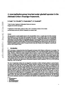
where Vud has been expressed in terms of the Cabibbo angle. In this particular case the Wilson Coefficient is equal unity and the local operator, the object between the square brackets, is given by a product of two V − A currents. This local operator is represented by the diagram

(b) in fig. 1. Equation (2.2) represents the Fermi theory for β-decays as formulated by Sudarshan and Marshak [9] and Feynman and Gell-Mann [10] forty years ago, except that in (2.2) the quark language has been used and following Cabibbo a small departure of Vud from unity has been incorporated. In this context the basic formula (2.1) can be regarded as a generalization of the Fermi Theory to include all known quarks and leptons as well as their strong and electroweak interactions as summarized by the Standard Model. It should be stressed that the formulation of weak decays in terms of effective Hamiltonians is very suitable for the inclusion of new physics effects. We will discuss this issue briefly later on.

d

u d

u

ν

e

W

ν

e

(a)

(b)

Figure 1: β-decay at the quark level in the full (a) and effective (b) theory. Now, I am aware of the fact that the formal operator language used here is hated by experimentalists and frequently disliked by more phenomenological minded theorists. Consequently the literature on weak decays, in particular on B-meson decays [11], is governed by Feynman diagram drawings with W-, Z- and top quark exchanges, rather than by the operators in (2.1). In the case of the β-decay we have the diagram (a) in fig. 1. Yet such Feynman diagrams with full W-propagators, Z-propagators and top-quark propagators really represent the situation at very short distance scales O(MW,Z , mt ), whereas the true picture

of a decaying hadron with masses O(mb , mc , mK ) is more properly described by effective

point-like vertices which are represented by the local operators Qi . The Wilson coefficients Ci can then be regarded as coupling constants associated with these effective vertices. Thus Hef f in (2.1) is simply a series of effective vertices multiplied by effective coupling

constants Ci . This series is known under the name of the operator product expansion (OPE) [1]-[4], [12]. Due to the interplay of electroweak and strong interactions the structure of the local operators (vertices) is much richer than in the case of the β-decay. They can be classified with respect to the Dirac structure, colour structure and the type of quarks and leptons relevant for a given decay. Of particular interest are the operators involving quarks only. They govern the non-leptonic decays. To be specific let us list the operators relevant for non-leptonic B–meson decays. They are: Current–Current : Q1 = (¯ cα bβ )V −A (¯ sβ cα )V −A

Q2 = (¯ cb)V −A (¯ sc)V −A

(2.3)

QCD–Penguins : Q3 = (¯ sb)V −A

X

(¯ q q)V −A

Q4 = (¯ sα bβ )V −A

X

(¯ qβ qα )V −A

q=u,d,s,c,b

q=u,d,s,c,b

2

(2.4)

X

Q5 = (¯ sb)V −A

(¯ q q)V +A

X

Q6 = (¯ sα bβ )V −A

(¯ qβ qα )V +A

(2.5)

q=u,d,s,c,b

q=u,d,s,c,b

Electroweak–Penguins : Q7 =

Q9 =

X 3 eq (¯ q q)V +A (¯ sb)V −A 2 q=u,d,s,c,b

Q8 =

X 3 eq (¯ q q)V −A (¯ sb)V −A 2 q=u,d,s,c,b

Q10 =

X 3 eq (¯ qβ qα )V +A (¯ sα bβ )V −A 2 q=u,d,s,c,b

(2.6)

X 3 eq (¯ qβ qα )V −A . (¯ sα bβ )V −A 2 q=u,d,s,c,b

(2.7)

Here, α and β are colour indices and eq denotes the electrical quark charges reflecting the electroweak origin of Q7 , . . . , Q10 . Q2 , Q3−6 and Q7,9 originate in the tree level W ± -exchange, gluon penguin and (γ, Z 0 )-penguin diagrams respectively. These are the diagrams a)–c) in fig. 2. To generate Q1 , Q8 and Q10 additional gluonic exchanges are needed. The operators given above have dimension six. Of interest are also operators of dimension five which are responsible for the B → sγ decay. They originate in the diagram d) in fig. 2 where γ and

the gluon are on-shell. They will be given in Section 7. In what follows we will neglect the higher dimensional operators as their contributions to weak decays are marginal. b

c

b

c

b

s W

W

g

u,c,t

W

u,c,t g

c

s

c

s

q

q

(a) b

(b) b

s

b

s

s W

u,c,t

W u,c,t

W

u,c,t

t

t

γ,Z

γ,Z q

W

g,γ

q

q

q (d)

(c) d

b

b,s

s W

W u,c,t

t

u,c,t

t γ,Z

W b,s

l

d

l (f)

(e)

Figure 2: Typical Penguin and Box Diagrams. 3

Now what about the couplings Ci (µ) and the scale µ? The important point is that Ci (µ) summarize the physics contributions from scales higher than µ and due to asymptotic freedom of QCD they can be calculated in perturbation theory as long as µ is not too small. Ci include the top quark contributions and contributions from other heavy particles such as W, Z-bosons and charged Higgs particles or supersymmetric particles in the supersymmetric extensions of the Standard Model. At higher orders in the electroweak coupling the neutral Higgs may also contribute. Consequently Ci (µ) depend generally on mt and also on the masses of new particles if extensions of the Standard Model are considered. This dependence can be found by evaluating the box and penguin diagrams with full W-, Z-, top- and new particles exchanges shown in fig. 2 and properly including short distance QCD effects. The latter govern the µ-dependence of the couplings Ci (µ). The value of µ can be chosen arbitrarily. It serves to separate the physics contributions to a given decay amplitude into short-distance contributions at scales higher than µ and long-distance contributions corresponding to scales lower than µ. It is customary to choose µ to be of the order of the mass of the decaying hadron. This is O(mb ) and O(mc ) for B-decays

and D-decays respectively. In the case of K-decays the typical choice is µ = O(1 − 2 GeV )

instead of O(mK ), which is much too low for any perturbative calculation of the couplings Ci .

Now due to the fact that µ ≪ MW,Z , mt , large logarithms ln MW /µ compensate in the

evaluation of Ci (µ) the smallness of the QCD coupling constant αs and terms αns (ln MW /µ)n , αns (ln MW /µ)n−1 etc. have to be resummed to all orders in αs before a reliable result for Ci can

be obtained. This can be done very efficiently by means of the renormalization group methods [13, 14, 15]. Indeed solving the renormalization group equations for the Wilson coefficients Ci (µ) summs automatically large logarithms. The resulting renormalization group improved perturbative expansion for Ci (µ) in terms of the effective coupling constant αs (µ) does not involve large logarithms and is more reliable. It should be stressed at this point that the construction of the effective Hamiltonian Hef f

by means of the operator product expansion and the renormalization group methods can be done fully in the perturbative framework. The fact that the decaying hadrons are bound states of quarks is irrelevant for this construction. Consequently the coefficients Ci (µ) are independent of the particular decay considered in the same manner in which the usual gauge couplings are universal and process independent. Having constructed the effective Hamiltonian we can proceed to evaluate the decay amplitudes. An amplitude for a decay of a given meson M = K, B, .. into a final state

4

F = πν ν¯, ππ, DK is simply given by GF X i A(M → F ) = hF |Hef f |M i = √ VCKM Ci (µ)hF |Qi (µ)|M i, 2 i

(2.8)

where hF |Qi (µ)|M i are the hadronic matrix elements of Qi between M and F. As indicated

in (2.8) these matrix elements depend similarly to Ci (µ) on µ. They summarize the physics contributions to the amplitude A(M → F ) from scales lower than µ.

We realize now the essential virtue of OPE: it allows to separate the problem of calcu-

lating the amplitude A(M → F ) into two distinct parts: the short distance (perturbative) calculation of the couplings Ci (µ) and the long-distance (generally non-perturbative) calcu-

lation of the matrix elements hQi (µ)i. The scale µ, as advertised above, separates then the

physics contributions into short distance contributions contained in Ci (µ) and the long distance contributions contained in hQi (µ)i. By evolving this scale from µ = O(MW ) down to lower values one simply transforms the physics contributions at scales higher than µ from the

hadronic matrix elements into Ci (µ). Since no information is lost this way the full amplitude cannot depend on µ. Therefore the µ-dependence of the couplings Ci (µ) has to cancel the µdependence of hQi (µ)i. In other words it is a matter of choice what exactly belongs to Ci (µ)

and what to hQi (µ)i. This cancellation of µ-dependence involves generally several terms in

the expansion in (2.8).

Clearly, in order to calculate the amplitude A(M → F ), the matrix elements hQi (µ)i have

to be evaluated. Since they involve long distance contributions one is forced in this case to use non-perturbative methods such as lattice calculations, the 1/N expansion (N is the number of colours), QCD sum rules, hadronic sum rules, chiral perturbation theory and so on. In the case of certain B-meson decays, the Heavy Quark Effective Theory (HQET) turns out to be a useful tool. Needless to say, all these non-perturbative methods have some limitations. Consequently the dominant theoretical uncertainties in the decay amplitudes reside in the matrix elements hQi (µ)i.

The fact that in most cases the matrix elements hQi (µ)i cannot be reliably calculated at

present, is very unfortunate. One of the main goals of the experimental studies of weak decays

i is the determination of the CKM factors VCKM and the search for the physics beyond the

Standard Model. Without a reliable estimate of hQi (µ)i this goal cannot be achieved unless

these matrix elements can be determined experimentally or removed from the final measurable quantities by taking the ratios or suitable combinations of amplitudes or branching ratios. However, this can be achieved only in a handful of decays and generally one has to face directly the calculation of hQi (µ)i.

Now in the case of semi-leptonic decays, in which there is at most one hadron in the

final state, the chiral perturbation theory in the case of K-decays and HQET in the case of 5

B-decays have already provided useful estimates of the relevant matrix elements. This way it was possible to achieve satisfactory determinations of the CKM elements Vus and Vcb in K → πeν and B → D∗ eν respectively. Similarly certain rare decays like K → πν ν¯ and B → µ¯ µ can be calculated very reliably.

The case of non-leptonic decays in which the final state consists exclusively out of hadrons

is a completely different story. Here even the matrix elements entering the simplest decays, the two-body decays like K → ππ, D → Kπ or B → DK cannot be calculated in QCD reliably at present. More promising in this respect is the evaluation of hadronic matrix ¯ 0 and B 0 − B ¯ 0 mixings. elements relevant for K 0 − K d,s d,s Returning to the Wilson coefficients Ci (µ) it should be stressed that similar to the effective

coupling constants they do not depend only on the scale µ but also on the renormalization scheme used: this time on the scheme for the renormalization of local operators. That the local operators undergo renormalization is not surprising. After all they represent effective vertices and as the usual vertices in a field theory they have to be renormalized when quantum corrections like QCD or QED corrections are taken into account. As a consequence of this, the hadronic matrix elements hQi (µ)i are renormalization scheme dependent and this

scheme dependence must be cancelled by the one of Ci (µ) so that the physical amplitudes are renormalization scheme independent. Again, as in the case of the µ-dependence, the cancellation of the renormalization scheme dependence involves generally several terms in the expansion (2.8). Now the µ and the renormalization scheme dependences of the couplings Ci (µ) can be evaluated efficiently in the renormalization group improved perturbation theory. Unfortunately the incorporation of these dependences in the non-perturbative evaluation of the matrix elements hQi (µ)i remains as an important challenge and most of the non-perturbative methods

on the market are insensitive to these dependences. The consequence of this unfortunate situation is obvious: the resulting decay amplitudes are µ and renormalization scheme de-

pendent which introduces potential theoretical uncertainty in the predictions. On the other hand in certain decays these dependences can be put under control. So far I have discussed only exclusive decays. It turns out that in the case of inclusive decays of heavy mesons, like B-mesons, things turn out to be easier. In an inclusive decay one sums over all (or over a special class) of accessible final states so that the amplitude for an inclusive decay takes the form: GF X i A(B → X) = √ VCKM Ci (µ)hf |Qi (µ)|Bi . 2 f ∈X

(2.9)

At first sight things look as complicated as in the case of exclusive decays. It turns out, however, that the resulting branching ratio can be calculated in the expansion in inverse 6

powers of mb with the leading term described by the spectator model in which the B-meson decay is modelled by the decay of the b-quark: Br(B → X) = Br(b → q) + O(

1 ). m2b

(2.10)

This formula is known under the name of the Heavy Quark Expansion (HQE) [16]-[18]. Since the leading term in this expansion represents the decay of the quark, it can be calculated in perturbation theory or more correctly in the renormalization group improved perturbation theory. It should be realized that also here the basic starting point is the effective Hamiltonian (2.1) and that the knowledge of the couplings Ci (µ) is essential for the evaluation of the leading term in (2.10). But there is an important difference relative to the exclusive case: the matrix elements of the operators Qi can be ”effectively” evaluated in perturbation theory. This means, in particular, that their µ and renormalization scheme dependences can be evaluated and the cancellation of these dependences by those present in Ci (µ) can be explicitly investigated. Clearly in order to complete the evaluation of Br(B → X) also the remaining terms in

(2.10) have to be considered. These terms are of a non-perturbative origin, but fortunately

they are suppressed by at least two powers of mb . They have been studied by several authors in the literature with the result that they affect various branching ratios by less than 10% and often by only a few percent. Consequently the inclusive decays give generally more precise theoretical predictions at present than the exclusive decays. On the other hand their measurements are harder. There is of course an important theoretical issue related to the validity of HQE in (2.10) which appear in the literature under the name of quark-hadron duality. I will not discuss it here. Recent discussions of this issue can be found in [19]. We have learned now that the matrix elements of Qi are easier to handle in inclusive decays than in the exclusive ones. On the other hand the evaluation of the couplings Ci (µ) is equally difficult in both cases although as stated above it can be done in a perturbative framework. Still in order to achieve sufficient precision for the theoretical predictions it is desirable to have accurate values of these couplings. Indeed it has been realized at the end of the eighties that the leading term (LO) in the renormalization group improved perturbation theory, in which the terms αns (ln MW /µ)n are summed, is generally insufficient and the inclusion of next-to-leading corrections (NLO) which correspond to summing the terms αns (ln MW /µ)n−1 is necessary. In particular, unphysical left-over µ-dependences in the decay amplitudes and branching ratios resulting from the truncation of the perturbative series are considerably reduced by including NLO corrections. These corrections are known by now for the most important and interesting decays and will be briefly reviewed below.

7

3

Penguin–Box Expansion and OPE

The FCNC decays, in particular rare and CP violating decays are governed by various penguin and box diagrams with internal top quark and charm quark exchanges. Some examples are shown in fig. 2. These diagrams can be evaluated in the full theory and are summarized by a set of basic universal (process independent) mt -dependent functions Fr (xt ) [20] where 2 . Explicit expressions for these functions can be found in [21, 22, 23]. xt = m2t /MW

It is useful to express the OPE formula (2.8) directly in terms of the functions Fr (xt ) [25]. To this end we rewrite the A(M → F ) in (2.8) as follows X GF ˆki (µ, MW ) Ci (MW ), A(M → F ) = √ VCKM hF | Ok (µ) | M i U 2 i,k

(3.11)

ˆkj (µ, MW ) is the renormalization group transformation from MW down to µ. Explicit where U formula for this transformation will be given below. In order to simplify the presentation we i have removed the index “i” from VCKM

Now Ci (MW ) are linear combinations of the basic functions Fr (xt ) so that we can write Ci (MW ) = ci +

X

hir Fr (xt )

(3.12)

r

where ci and hir are mt -independent constants. Inserting (3.12) into (3.11) and summing over i and k we find A(M → F ) = P0 (M → F ) +

X r

Pr (M → F ) Fr (xt ),

(3.13)

with ˆki (µ, MW )ci , hF | Ok (µ) | M i U

(3.14)

ˆki (µ, MW )hir , hF | Ok (µ) | M i U

(3.15)

P0 (M → F ) =

X

Pr (M → F ) =

X

i,k

i,k

√ where we have suppressed the overall factor (GF / 2)VCKM . I would like to call (3.13) Penguin-Box Expansion (PBE) [25]. The coefficients P0 and Pr are process dependent. This process dependence enters through hF | Ok (µ) | M i. In certain cases like K → πν ν¯ these matrix elements are very simple implying simple formulae for the coefficients P0 and Pr . In other situations, like ε′ /ε, this is

not the case. Originally PBE was designed to expose the mt -dependence of FCNC processes [25]. After the top quark mass has been measured precisely this role of PBE is less important. On the other hand, PBE is very well suited for the study of the extentions of the Standard Model in which new particles are exchanged in the loops. We know already that these particles are 8

heavier than W-bosons and consequently they can be integrated out together with the weak bosons and the top quark. If there are no new local operators the mere change is to modify the functions Fr (xt ) which now acquire the dependence on the masses of new particles such as charged Higgs particles and supersymmetric particles. The process dependent coefficients P0 and Pr remain unchanged. This is particularly useful as the most difficult part is the ˆkj (µ, MW ) and of the hadronic matrix elements, both contained in these evaluation of U coefficients. However, if new effective operators with different Dirac and colour structures are present the values of P0 and Pr are modified. Examples of the applications of PBE to physics beyond the Standard Model can be found in [26, 27, 28]. The universality of the functions Fr (xt ) can be violated partly when QCD corrections to one loop penguin and box diagrams are included. For instance in the case of semi-leptonic FCNC transitions there is no gluon exchange in a Z 0 -penguin diagram parallel to the Z 0 propagator but such an exchange takes place in non-leptonic decays in which the bottom line is a quark-line. Thus the general universality of Fr (xt ) present at one loop level is reduced to two universality classes relevant for semi-leptonic and non-leptonic transitions. However, the O(αs ) corrections to the functions Fr (xt ) are generally rather small when the top quark

mass mt (mt ) is used and consequently the inclusion of QCD effects plays mainly the role in reducing various µ-dependences. In order to see the general structure of A(M → F ) more transparently let us write it as

follows:

A(M → F ) = BM →F VCKM ηQCD F (xt ) + Charm

(3.16)

where the first term represents the internal top quark contribution and ”Charm” stands for remaining contributions, in particular those with internal charm quark exchanges. F (xt ) represents one of the universal functions and ηQCD the corresponding short distance QCD corrections. The parameter BM →F represents the relevant hadronic matrix element, which can only be calculated by means of non-perturbative methods. However, in certain lucky situations BM →F can be extracted from well measured leading decays and when it enters also other decays, the latter are then free from hadronic uncertainties and offer very useful means for extraction of CKM parameters. One such example is the decay K + → π + ν ν¯ for which one has

+

+

Br(K → π ν ν¯) =

"

α2QED Br(K + → π 0 e+ ν) 4

2 2π 2 sin θ Vus W

#



2

t c · Vts∗ Vtd ηQCD F (xt ) + Vcs∗ Vcd ηQCD F (xc )

(3.17)

The factor in square brackets stands for the ”B − f actor” in (3.16), which is given in terms

of well measured quantities. Since Vcs , Vcd and Vts are already rather well determined and 9

i F (xi ) and ηQCD can be calculated in perturbation theory, the element Vtd can be extracted

from Br(K + → π + ν ν¯) without essentially any theoretical uncertainties. We will be more

specific about this in Section 7.

4

Motivations for NLO Calculations

Going beyond the LO approximation for Ci (µ) is certainly an important but a non-trivial step. For this reason one needs some motivations to perform this step. Here are the main reasons for going beyond LO: • The NLO is first of all necessary to test the validity of the renormalization group improved perturbation theory.

• Without going to NLO the QCD scale ΛM S [29] extracted from various high energy processes cannot be used meaningfully in weak decays.

• Due to renormalization group invariance the physical amplitudes do not depend on the scales µ present in αs or in the running quark masses, in particular mt (µ), mb (µ) and mc (µ). However, in perturbation theory this property is broken through the truncation of the perturbative series. Consequently one finds sizable scale ambiguities in the leading order, which can be reduced considerably by going to NLO. • The Wilson Coefficients are renormalization scheme dependent quantities. This scheme dependence appears first at NLO. For a proper matching of the short distance contributions to the long distance matrix elements obtained from lattice calculations it is essential to calculate NLO. The same is true for inclusive heavy quark decays in which the hadron decay can be modeled by a decay of a heavy quark and the matrix elements of Qi can be effectively calculated in an expansion in 1/mb . • In several cases the central issue of the top quark mass dependence is strictly a NLO effect.

5

General Structure of Wilson Coefficients

We will give here a formula for the Wilson coefficient C(µ) of a single operator Q including NLO corrections. The case of several operators which mix under renormalization is much more complicated. Explicit formulae are given in [21, 23]. C(µ) is given by C(µ) = U (µ, MW )C(MW ) 10

(5.18)

where U (µ, MW ) = exp

"Z

γQ (gs′ ) dg′ β(gs′ ) gs (MW ) gs (µ)

#

(5.19)

is the evolution function, which allows to calculate C(µ) once C(MW ) is known. The latter can be calculated in perturbation theory in the process of integrating out W ± , Z 0 and top quark fields. Details can be found in [21, 23]. Next γQ is the anomalous dimension of the operator Q and β(gs ) is the renormalization group function which governs the evolution of the QCD coupling constant αs (µ). At NLO we have

αs (MW ) B 4π

C(MW ) = 1 +

γQ (αs ) =

2

(5.21)

gs5 gs3 − β 1 16π 2 (16π 2 )2

(5.22)

(0) αs γQ

4π

β(gs ) = −β0

(5.20)

+

(1) γQ



αs 4π

Inserting the last two formulae into (5.19) and expanding in αs we find αs (µ) U (µ, MW ) = 1 + J 4π 

with



αs (MW ) αs (µ)

d 

αs (MW ) J 1− 4π

(1)



(5.23)

(0)

γQ d J = β1 − β0 2β0

d=

γQ

2β0

.

(5.24)

Inserting (5.23) and (5.20) into (5.18) we find an important formula for C(µ) in the NLO approximation: 

C(µ) = 1 +

6

αs (µ) J 4π



αs (MW ) αs (µ)

d 

1+

αs (MW ) (B − J) . 4π 

(5.25)

Status of NLO Calculations

Since the pioneering leading order calculations of Wilson coefficients for current–current [5, 6] and penguin operators [30], enormous progress has been made, so that at present most of the decay amplitudes are known at the NLO level. We list all existing NLO calculations for weak decays in table 1. In addition to the calculations in the Standard Model we list the calculations in two-Higgs doublet models and supersymmetry. In table 2 we list references to calculations of two-loop electroweak contributions to rare decays. The latter calculations allow to reduce scheme and scale dependences related to the definition of electroweak parameters like sin2 θW , αQED , etc. Next, useful techniques for three-loop calculations can be found in [77] and a very 11

general discussion of the evanescent operators including earlier references is presented in [78]. Further details on these calculations can be found in the orignal papers, in the review [21] and in the Les Houches lectures [23]. Some of the implications of these calculations will be analyzed briefly in subsequent sections.

7 7.1

Applications: News Preliminaries

There is a vast literature on the applications of NLO calculations listed in table 1. As they are already reviewed in detail in [21, 22, 23] there is no point to review them here again. I will rather discuss briefly some of the most important applications in general terms. This will also give me the opportunity to update some of the numerical results presented in [23]. ¯s0 mixing This update is related mainly to the improved experimental lower bound on Bs0 − B

((∆M )s > 12.4/ps) and a slight increase in |Vub |/|Vcb |: 0.091 ± 0.016, both presented at the last Rochester Conference in Vancouver [79].

A=(ρ,η) α ρ+i η

1−ρ−i η

γ

β

C=(0,0)

B=(1,0) Figure 3: Unitarity Triangle.

7.2

Unitarity Triangle

The standard analysis of the unitarity triangle (see fig. 3) uses the values of |Vus |, |Vcb |, |Vub /Vcb | extracted from tree level K- and B- decays, the indirect CP-violation in KL → ππ ¯ 0 mixings described by the mass differences represented by the parameter ε and the B 0 − B d,s

d,s

(∆M )d,s . From this analysis follows the allowed range for (¯ ̺, η¯) describing the apex of the unitarity triangle. Here [81] ̺¯ = ̺(1 −

λ2 ), 2

η¯ = η(1 − 12

λ2 ). 2

(7.26)

where λ, ̺ and η are Wolfenstein parameters [82] with |Vus | = λ = 0.22. We have in particular Vub = λ|Vcb |(̺ − iη),

Vtd = λ|Vcb |(1 − ̺¯ − i¯ η ).

(7.27)

η 6= 0 is responsible for CP violation in the Standard Model.

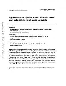
The allowed region for (¯ ̺, η¯) is presented in fig. 4. It is the shaded area on the right

hand side of the solid circle which represents the upper bound for (∆M )d /(∆M )s . The hyperbolas give the constraint from ε and the two circles centered at (0, 0) the constraint from |Vub /Vcb |. The white areas between the lower ε-hyperbola and the shaded region are ¯ 0 mixing. We observe that the region ̺¯ < 0 is practically excluded. The excluded by Bd0 − B d

main remaining theoretical uncertainties in this analysis are the values of non-perturbative √ √ √ parameters: BK in ε, FBd Bd in (∆M )d and ξ = FBs Bs /FBd Bd in (∆M )d /(∆M )s . I √ have used BK = 0.80 ± 0.15, FBd Bd = 200 ± 40 MeV and ξmax = 1.2. On the experimental side |Vub /Vcb | and (∆M )s should be improved.

−1

(ξ,(∆M)s)=(1.2,12.4ps )

0.8 −1

(1.2,15ps )

0.6 −1

(1.2,25ps )

η

|

0.4

0.2

0.0

−0.6

−0.4

−0.2

0.0 − ρ

0.2

0.4

0.6

Figure 4: Unitarity Triangle 1998. From this analysis we extract |Vtd | = (8.6 ± 1.6) · 10−3 ,

Im(Vts∗ Vtd ) = (1.38 ± 0.33) · 10−4

(7.28)

and sin 2β = 0.71 ± 0.13,

7.3

sin γ = 0.83 ± 0.17

(7.29)

ε′ /ε

ε′ /ε is the ratio of the direct and indirect CP violation in KL → ππ. A measurement of

a non-vanishing value of ε′ /ε would give the first signal for the direct CP violation ruling 13

out the superweak models [83]. In the Standard Model ε′ /ε is governed by QCD penguins and electroweak (EW) penguins. The corresponding operators are given in (2.4)-(2.7). With increasing mt the EW penguins become increasingly important [84, 85], and entering ε′ /ε with the opposite sign to QCD penguins suppress this ratio for large mt . For mt ≈ 200 GeV

the ratio can even be zero [85]. Because of this strong cancellation between two dominant contributions and due to uncertainties related to hadronic matrix elements of the relevant local operators, a precise prediction of ε′ /ε is not possible at present. A very simplified formula (not to be used for any serious numerical analysis) which exhibits

main uncertainties is given as follows "

ε′ ηλ|Vcb |2 = 15 · 10−4 ε 1.3 · 10−4

#

120 M eV ms (2 GeV)

2

 

(4)

ΛMS 300 MeV

0.8 

[B6 − Z(xt )B8 ]

(7.30)

where Z(xt ) ≈ 0.18(mt /MW )1.86 represents the leading mt -dependence of EW penguins. B6 and B8 represent the hadronic matrix elements of the dominant QCD-penguin operator

Q6 and the dominant electroweak penguin operator Q8 (see (2.5) and (2.6)) respectively. Together with ms (2 GeV) the values of these parameters constitute the main theoretical uncertainty in evaluating ε′ /ε. Present status of ms , B6 and B8 is reviewed in [86, 23]. Roughly one has B6 = 1.0 ± 0.2 and B8 = 0.7 ± 0.2. Taking these values, η of fig. 4 and |Vcb | = 0.040 ± 0.003, I find:

  (5.7 ± 3.6) · 10−4 , ε′ /ε =  (9.1 ± 5.7) · 10−4 ,

ms (2 GeV) = 130 ± 20 MeV

ms (2 GeV) = 110 ± 20 MeV.

(7.31)

where the chosen values for ms are in the ball park of various QCD sum rules and lattice estimates [86]. This should be compared with the result of NA31 collaboration at CERN which finds (ε′ /ε) = (23 ± 7) · 10−4 [87] and the value of E731 at Fermilab, (ε′ /ε) = (7.4 ±

5.9) · 10−4 [88].

The Standard Model expectations are closer to the Fermilab result, but due to large

theoretical and experimental errors no firm conclusion can be reached at present. The new improved data from CERN and Fermilab in 1999 and later from DAΦNE should shed more light on ε′ /ε. In this context improved estimates of B6 , B8 and ms are clearly desirable.

7.4

B → Xs γ

A lot of efforts have been put into predicting the branching ratio for the inclusive decay B → Xs γ including NLO QCD corrections and higher order electroweak corrections. The

relevant references are given in table 1 and in [23], where details can be found. The final

14

result of these efforts can be summarized by Br(B → Xs γ)th = (3.30 ± 0.15(scale) ± 0.26(par)) · 10−4

(7.32)

where the first error represents residual scale dependences and the second error is due to uncertainties in input parameters. The main achievement is the reduction of the scale dependence through NLO calculations, in particular those given in [61] and [40]. In the leading order the corresponding error would be roughly ±0.6 [89, 90].

The theoretical result in (7.32) should be compared with experimental data: Br(B → Xs γ)exp

  (3.15 ± 0.35 ± 0.41) · 10−4 , =  (3.11 ± 0.80 ± 0.72) · 10−4 ,

CLEO ALEPH,

(7.33)

which implies the combined branching ratio:

Br(B → Xs γ)exp = (3.14 ± 0.48) · 10−4

(7.34)

Clearly, the Standard Model result agrees well with the data. In order to see whether any new physics can be seen in this decay, the theoretical and in particular experimental errors should be reduced. This is certainly a very difficult task. Most recent analyses of B → Xs γ in supersymmetric models and two–Higgs doublet models are listed in table 1.

7.5

KL → π 0 ν ν¯ and K + → π + ν ν¯

KL → π 0 ν ν¯ and K + → π + ν ν¯ are the theoretically cleanest decays in the field of rare Kdecays. KL → π 0 ν ν¯ is dominated by short distance loop diagrams (Z-penguins and box

diagrams) involving the top quark. K + → π + ν ν¯ receives additional sizable contributions

from internal charm exchanges. The great virtue of KL → π 0 ν ν¯ is that it proceeds almost

exclusively through direct CP violation [91] and as such is the cleanest decay to measure this important phenomenon. It also offers a clean determination of the Wolfenstein parameter η and in particular offers the cleanest measurement of ImVts∗ Vtd [92]. K + → π + ν ν¯ is CP conserving and offers a clean determination of |Vtd |. Due to the presence of the charm

contribution and the related mc dependence it has a small scale uncertainty absent in KL →

π 0 ν ν¯.

The next-to-leading QCD corrections [49, 50, 53, 51, 52] to both decays considerably reduced the theoretical uncertainty due to the choice of the renormalization scales present in the leading order expressions, in particular in the charm contribution to K + → π + ν ν¯.

Since the relevant hadronic matrix elements of the weak currents entering K → πν ν¯ can be related using isospin symmetry to the leading decay K + → π 0 e+ ν, the resulting theoretical

expressions for Br( KL → π 0 ν ν¯) and Br(K + → π + ν ν¯) are only functions of the CKM 15

parameters, the QCD scale ΛMS and the quark masses mt and mc . The isospin braking corrections have been calculated in [93]. The long distance contributions to K + → π + ν ν¯ have

been considered in [94] and found to be very small: a few percent of the charm contribution to the amplitude at most, which is safely neglegible. The long distance contributions to KL → π 0 ν ν¯ are negligible as well [95].

The explicit expressions for Br(K + → π + ν ν¯) and Br(KL → π 0 ν ν¯) can be found in

[21, 22, 23]. Here we give approximate expressions in order to exhibit various dependences:

+

+

−10

Br(K → π ν ν¯) = 0.7 · 10

"

|Vtd | 0.010

2 

Br(KL → π 0 ν ν¯) = 3.0 · 10−11



| Vcb | 0.040

η 0.39

2 

2 

mt (mt ) 170 GeV

mt (mt ) 170 GeV

2.3

2.3 

+ cc + tc

| Vcb | 0.040

#

4

(7.35)

(7.36)

where in (7.35) we have shown explicitly only the pure top contribution. The impact of NLO calculations is the reduction of scale uncertainties in Br(K + → π + ν ν¯)

from ±23% to ±7%. This corresponds to the reduction in the uncertainty in the determination

of |Vtd | from ±14% to ±4%. The remaining scale uncertainties in Br(KL → π 0 ν ν¯) and in

the determination of η are fully negligible.

Updating the analysis of [23] one finds [52]: Br(K + → π + ν ν¯) = (8.2 ± 3.2) · 10−11

,

Br(KL → π 0 ν ν¯) = (3.1 ± 1.3) · 10−11

(7.37)

where the errors come dominantly from the uncertainties in the CKM parameters. As stressed in [92] simultaneous measurements of Br(K + → π + ν ν¯) and Br(KL → π 0 ν ν¯)

should allow a clean determination of the unitarity triangle as shown in fig. 5. In particular the measurements of these branching ratios with an error of ±10% will determine |Vtd |, ImVts∗ Vtd and sin 2β with an accuraccy of ±10%, ±5% and ±0.05 respectively. The comparision of this determination of sin 2β with the one by means of the CP-asymmetry in B → ψKS should offer a very good test of the Standard Model. Experimentally we have [96] BR(K + → π + ν ν¯) = (4.2+9.7−3.5) · 10−10

(7.38)

BR(KL → π 0 ν ν¯) < 1.6 · 10−6 .

(7.39)

and the bound [97]

Moreover from (7.38) and isospin symmetry one has [98] BR(KL → π 0 ν ν¯) < 6.1 · 10−9 .

The central value in (7.38) is by a factor of 4 above the Standard Model expectation

but in view of large errors the result is compatible with the Standard Model. The analysis 16

( %;  )

 KL

K+

! o 

! +



(0; 0)

(1; 0)

Figure 5: Unitarity triangle from K → πν ν¯. of additional data on K + → π + ν ν¯ present on tape at BNL787 should narrow this range in the near future considerably. In view of the clean character of this decay a measurement

of its branching ratio at the level of 2 · 10−10 would signal the presence of physics beyond the Standard Model [52]. The Standard Model sensitivity is expected to be reached at AGS around the year 2000 [99]. Also Fermilab with the Main Injector could measure this decay [100]. The present upper bound on Br(KL → π 0 ν ν¯) is about five orders of magnitude above

the Standard Model expectation (7.37). FNAL-E799 expects to reach the accuracy O(10−8 )

and a very interesting new experiment at Brookhaven (BNL E926) [99] expects to reach the single event sensitivity 2 · 10−12 allowing a 10% measurement of the expected branching ratio.

There are furthermore plans to measure this gold-plated decay with comparable sensitivity at Fermilab [101] and KEK [102].

8

Summary

We have given a general description of OPE and Renormalization Group techniques as applied to weak decays of mesons. Further details can be found in [21, 22, 23, 103]. One of the outstanding and important challanges for theorists in this field is a quantitative description of non–leptonic meson decays. In the field of K–decays this is in particular the case of the ∆I = 1/2 rule for which some progress has been made in [104]. In the field of B– decays progress in a quantitative description of two–body decays is very desirable in view of forthcoming B-physics experiments at Cornell, SLAC, KEK, DESY, FNAL and later at LHC. 17

Recent reviews on non-leptonic two-body decays are given in [105, 106, 107] where further references can be found. I would like to thank Peter Breitenlohner, Dieter Maison and Julius Wess for inviting me to such a pleasant symposium.

References [1] K.G. Wilson, Phys. Rev. 179 (1969) 1499; [2] W. Zimmermann, in Proc. 1970 Brandeis Summer Institute in Theor. Phys, (eds. S. Deser, M. Grisaru and H. Pendleton), MIT Press, 1971, p.396; [3] K.G. Wilson and W. Zimmermann, Comm. Math. Phys. 24 (1972) 87. [4] W. Zimmermann, Ann. Phys. 77 (1973) 570. [5] M.K. Gaillard and B.W. Lee, Phys. Rev. Lett. 33 (1974) 108. [6] G. Altarelli and L. Maiani, Phys. Lett. B 52 (1974) 351. [7] N. Cabibbo, Phys. Rev. Lett. 10 (1963) 531. [8] M. Kobayashi and K. Maskawa, Prog. Theor. Phys. 49 (1973) 652. [9] E.C.G. Sudarshan and R.E. Marshak, Proc. Padua-Venice Conf. on Mesons and Recently Discovered Particles (1957). [10] R.P. Feynman and M. Gell-Mann, Phys. Rev. 109 (1958) 193. [11] D. Zeppenfeld, Z. Phys. C 8 (1981) 77; L.L. Chau, Phys. Rev. D 43 (1991) 2176; M. Gronau, J.L. Rosner and D. London, Phys. Rev. Lett. 73 (1994) 21; O.F. Hernandez, M. Gronau, J.L. Rosner and D. London, Phys. Lett. B 333 (1994) 500, Phys. Rev. D 50 (1994) 4529. [12] E. Witten, Nucl. Phys. B 120 (1977) 189. [13] E.C.G. Stueckelberg and A. Petermann, Helv. Phys. Acta 26 (1953) 499; M. Gell–Mann and F.E. Low, Phys. Rev. 95 (1954) 1300; N.N. Bogoliubov and D.V. Shirkov, Dokl. Acad. Nauk SSSR 103 (1955) 203, 391; L.V. Ovsyannikov, Dokl. Acad. Nauk SSSR 109 (1956) 1112; K. Symanzik, Comm. Math. Phys. 18 (1970) 227; C.G. Callan Jr, Phys. Rev. D 2 (1970) 1541. [14] G. ’t Hooft, Nucl. Phys. B 61 (1973) 455. 18

[15] S. Weinberg, Phys. Rev. D 8 (1973) 3497. [16] J. Chay, H. Georgi and B. Grinstein, Phys. Lett. B 247 (1990) 399. [17] I.I. Bigi, N.G. Uraltsev and A.I. Vainshtein, Phys. Lett. B 293 (1992) 430 [E: B 297 (1993) 477]. I.I. Bigi, M.A. Shifman, N.G. Uraltsev and A.I. Vainshtein, Phys. Rev. Lett. 71 (1993) 496; B. Blok, L. Koyrakh, M.A. Shifman and A.I. Vainshtein, Phys. Rev. D 49 (1994) 3356 [E: D 50 (1994) 3572]. [18] A.V. Manohar and M.B. Wise, Phys. Rev. D 49 (1994) 1310. [19] Z. Ligeti and A.V. Manohar, Phys. Lett. B 433 (1998) 396; I. Bigi, M. Shifman, N. Uraltsev and A. Vainshtein, hep-ph/9805241; B.Grinstein and R.F. Lebed, hepph/9805404; N. Isgur, hep-ph/9811377. [20] T. Inami and C.S. Lim, Progr. Theor. Phys. 65 (1981) 297. [21] G. Buchalla, A.J. Buras and M. Lautenbacher, Rev. Mod. Phys 68 (1996) 1125. [22] A.J. Buras and R. Fleischer, hep-ph/9704376, page 65 in [24]. [23] A.J. Buras, hep-ph/9806471, to appear in Probing the Standard Model of Particle Interactions, eds. F. David and R. Gupta (Elsevier Science B.V., Amsterdam, 1998). [24] A.J. Buras and M. Lindner, Heavy Flavours II, World Scientific, 1998. [25] G. Buchalla, A.J. Buras and M.K. Harlander, Nucl. Phys. B 349 (1991) 1. [26] G. Buchalla, A.J. Buras, M.K. Harlander, M.E. Lautenbacher and C. Salazar, Nucl. Phys. B 355 (1991) 305. [27] P. Cho, M. Misiak and D. Wyler, Phys. Rev. D 54 (1996) 3329. [28] A. Ali, Th. Mannel and Ch. Greub, Zeit. Phys. C 67 (1995) 417. [29] W.A. Bardeen, A.J. Buras, D.W. Duke and T. Muta, Phys. Rev. D 18 (1978) 3998. [30] A.I. Vainshtein, V.I. Zakharov, and M.A. Shifman, JTEP 45 (1977) 670. F. Gilman and M.B. Wise, Phys. Rev. D 20 (1979) 2392; B. Guberina and R. Peccei, Nucl. Phys. B 163 (1980) 289. [31] G. Altarelli, G. Curci, G. Martinelli and S. Petrarca, Nucl. Phys. B 187 (1981) 461. [32] A.J. Buras and P.H. Weisz, Nucl. Phys. B 333 (1990) 66.

19

[33] A.J. Buras, M. Jamin, M.E. Lautenbacher and P.H. Weisz, Nucl. Phys. B 370 (1992) 69; Nucl. Phys. B 400 (1993) 37. [34] A.J. Buras, M. Jamin and M.E. Lautenbacher, Nucl. Phys. B 400 (1993) 75. [35] A.J. Buras, M. Jamin and M.E. Lautenbacher, Nucl. Phys. B 408 (1993) 209. [36] M. Ciuchini, E. Franco, G. Martinelli and L. Reina, Phys. Lett. B 301 (1993) 263. [37] M. Ciuchini, E. Franco, G. Martinelli and L. Reina, Nucl. Phys. B 415 (1994) 403. [38] K. Chetyrkin, M. Misiak and M¨ unz, Nucl. Phys. B520 (1998) 279. [39] M.Misiak and M. M¨ unz, Phys. Lett. B344 (1995) 308. [40] K.G. Chetyrkin, M. Misiak and M. M¨ unz, Phys. Lett. B400 (1997) 206; Erratum ibid. B425 (1998) 414. [41] G. Buchalla, Nucl. Phys. B 391 (1993) 501. [42] E. Bagan, P.Ball, V.M. Braun and P.Gosdzinsky, Nucl. Phys. B 432 (1994) 3; E. Bagan et al., Phys. Lett. B 342 (1995) 362; B 351 (1995) 546. [43] A. Lenz, U. Nierste and G. Ostermaier, Phys. Rev. D 56 (1997) 7228. [44] M. Jamin and A. Pich, Nucl. Phys. B425 (1994) 15. [45] S. Herrlich and U. Nierste, Nucl. Phys. B419 (1994) 292. [46] A.J. Buras, M. Jamin, and P.H. Weisz, Nucl. Phys. B347 (1990) 491. [47] J. Urban, F. Krauss, U.Jentschura and G. Soff, Nucl. Phys. B523 (1998) 40. [48] S. Herrlich and U. Nierste, Phys. Rev. D52 (1995) 6505; Nucl. Phys. B476 (1996) 27. [49] G. Buchalla and A.J. Buras, Nucl. Phys. B 398 (1993) 285. [50] G. Buchalla and A.J. Buras, Nucl. Phys. B 400 (1993) 225. [51] M. Misiak and J. Urban, hep-ph/9901278. [52] G. Buchalla and A.J. Buras, hep-ph/9901288. [53] G. Buchalla and A.J. Buras, Nucl. Phys. B 412 (1994) 106. [54] G. Buchalla and A.J. Buras, Phys. Lett. B 336 (1994) 263. 20

[55] A. J. Buras, M. E. Lautenbacher, M. Misiak and M. M¨ unz, Nucl. Phys. B423 (1994) 349. [56] M. Misiak, Nucl. Phys. B393 (1993) 23; Erratum, Nucl. Phys. B439 (1995) 461. [57] A.J. Buras and M. M¨ unz, Phys. Rev. D 52 (1995) 186. [58] A. Ali, and C. Greub,

Z.Phys. C49 (1991) 431;

Phys. Lett. B259 (1991) 182;

Phys. Lett. B361 (1995) 146. [59] K. Adel and Y.P. Yao, Modern Physics Letters A8 (1993) 1679; Phys. Rev. D 49 (1994) 4945. [60] N. Pott, Phys. Rev. D 54 (1996) 938. [61] C. Greub, T. Hurth and D. Wyler, Phys. Lett. B380 (1996) 385; Phys. Rev. D 54 (1996) 3350; [62] C. Greub and T. Hurth, Phys. Rev. D 56 (1997) 2934; hep-ph/9809468. [63] A.J. Buras, A. Kwiatkowski and N. Pott, Phys. Lett. B 414 (1997) 157, Nucl. Phys. B 517 (1998) 353. [64] M. Ciuchini, G. Degrassi, P. Gambino and G.F. Giudice, Nucl. Phys. B 527 (1998) 21. [65] F.M. Borzumati and Ch. Greub, Phys. Rev. D 58 (1998) 07004; hep-ph/9809438. [66] P. Ciafaloni, A. Romanino, and A. Strumia, Nucl. Phys. B 524 (1998) 361. [67] M. Beneke, G. Buchalla, C. Greub, A. Lenz and U. Nierste, hep-ph/9808385. [68] M. Beneke, F. Maltoni and I.Z. Rothstein, hep-ph/9808360. [69] M. Ciuchini, E. Franco, V. Lubicz, G. Martineli, I. Scimeni and L. Silvestrini, Nucl. Phys. B 523 (1998) 501. [70] M. Ciuchini, et al. JHEP 9810 (1998) 008. [71] M. Ciuchini, G. Degrassi, P. Gambino and G.F. Giudice, Nucl. Phys. B 534 (1998) 3. [72] G. Buchalla and A.J. Buras, Phys. Rev. D57 (1998) 216. [73] A. Czarnecki and W.J. Marciano, Phys. Rev. Lett. 81 (1998) 277. [74] A. Strumia, Nucl. Phys. B532 (1998) 28. 21

[75] A.L. Kagan and M. Neubert, hep-ph/9805303. [76] P. Gambino, A. Kwiatkowski and N. Pott, hep-ph/9810400. [77] K. Chetyrkin, M. Misiak and M¨ unz, Nucl. Phys. B518 (1998) 473. [78] S. Herrlich and U. Nierste, Nucl. Phys. B 445 (1995) 39. [79] J. Alexander; D. Karlen; P. Rosnet; talks given at the 29th International Conference on High Energy Physics (ICHEP 98), Vancouver, Canada, 23-29 July 1998, to appear in the proceedings. [80] Particle Data Group, Phys. Rev. D 54 (1996) 1. [81] A.J. Buras, M.E. Lautenbacher and G. Ostermaier, Phys. Rev. D 50 (1994) 3433. [82] L. Wolfenstein, Phys. Rev. Lett. 51 (1983) 1945. [83] L. Wolfenstein, Phys. Rev. Lett. 13 (1964) 562. [84] J. M. Flynn and L. Randall, Phys. Lett. B224 (1989) 221; erratum ibid. Phys. Lett. B235 (1990) 412. [85] G. Buchalla, A. J. Buras, and M. K. Harlander, Nucl. Phys. B337 (1990) 313. [86] R. Gupta, hep-ph/9801412; R.S. Sharpe, hep-lat/9811006. [87] G. D. Barr et al., Phys. Lett. B317 (1993) 233. [88] L. K. Gibbons et al., Phys. Rev. Lett. 70 (1993) 1203. [89] A. Ali, and C. Greub, Z.Phys. C60 (1993) 433. [90] A. J. Buras, M. Misiak, M. M¨ unz and S. Pokorski, Nucl. Phys. B424 (1994) 374. [91] L. Littenberg, Phys. Rev. D39 (1989) 3322. [92] G. Buchalla and A.J. Buras, Phys. Lett. B333 (1994) 221; Phys. Rev. D54 (1996) 6782. [93] W. Marciano and Z. Parsa, Phys. Rev. D53, R1 (1996). [94] D. Rein and L.M. Sehgal, Phys. Rev. D39 (1989) 3325; J.S. Hagelin and L.S. Littenberg, Prog. Part. Nucl. Phys. 23 (1989) 1; M. Lu and M.B. Wise, Phys. Lett. B324 (1994) 461; S. Fajfer, Nuovo Cim. 110A (1997) 397; C.Q. Geng, I.J. Hsu and Y.C. Lin, Phys. Rev. D54 (1996) 877. 22

[95] G. Buchalla and G. Isidori, hep-ph/9806501. [96] S. Adler et al., Phys. Rev. Lett. 79, (1997) 2204. [97] J. Adams et al., hep-ex/9806007. [98] Y. Grossman, Y. Nir and R. Rattazzi, [hep-ph/9701231] in [24]; Y. Grossman and Y. Nir, Phys. Lett. B398 (1997) 163; [99] L. Littenberg and J. Sandweiss, eds., AGS2000, Experiments for the 21st Century, BNL 52512. [100] P. Cooper, M. Crisler, B. Tschirhart and J. Ritchie (CKM collaboration), EOI for measuring Br(K + → π + ν ν¯) at the Main Injector, Fermilab EOI 14, 1996. [101] K. Arisaka et al., KAMI conceptual design report, FNAL, June 1991. [102] T. Inagaki, T. Sato and T. Shinkawa, Experiment to search for the decay KL → π 0 ν ν¯ at KEK 12 GeV proton synchrotron, 30 Nov. 1991.

[103] R. Fleischer, Int. J. of Mod. Phys. A12 (1997) 2459. [104] W. A. Bardeen, A. J. Buras and J.-M. G´erard, Phys. Lett. B192 (1987) 138; A. Pich and E. de Rafael, Nucl. Phys. B358 (1991) 311; M. Neubert and B. Stech, Phys. Rev. D 44 (1991) 775; M. Jamin and A. Pich, Nucl. Phys. B425 (1994) 15; J. Kambor, J. Missimer and D. Wyler, Nucl. Phys. B346 (1990) 17; Phys. Lett. B261 (1991) 496; V. Antonelli, S. Bertolini, M. Fabrichesi, and E.I. Lashin, Nucl. Phys. B469 (1996) 181; J. Bijnens and J. Prades, hep-ph/9811472. [105] M. Neubert and B. Stech, [hep-ph/9705292], page 294 in [24]; B. Stech [hepph/9706384]; M.Neubert, Nucl. Phys. B ph/9801269]. [106] A.J. Buras and L. Silvestrini, hep-ph/9812392. [107] A. Ali, hep-ph/9812434.

23

(Proc. Suppl.) 64 (1998) 474, [hep-

Table 1: References to NLO Calculations Decay

Reference

∆F = 1 Decays current-current operators

[31, 32]

QCD penguin operators

[33, 35, 36, 37, 38]

electroweak penguin operators

[34, 35, 36, 37]

magnetic penguin operators

[39, 40]

Br(B)SL

[31, 41, 42, 43]

inclusive ∆S = 1 decays

[44]

Particle-Antiparticle Mixing η1

[45]

η2 , ηB

[46, 47]

η3

[48] Rare K- and B-Meson Decays

KL0 → π 0 ν ν¯, B → l+ l− , B K + → π + ν ν¯, KL → µ+ µ− K+

→

KL →

→ Xs ν ν¯

[49, 50, 51, 52] [53, 52]

π + µ¯ µ

[54]

π 0 e+ e−

[55]

B → Xs µ+ µ−

[56, 57]

B → Xs γ

[58]-[65]

∆ΓBs

[67]

inclusive B → Charmonium

[68]

B → Xs γ

[64, 66, 65]

Two-Higgs Doublet Models Supersymmetry

∆MK and εK

[69, 70]

B → Xs γ

[71]

Table 2: Electroweak Two-Loop Calculations Decay KL0

→

π 0 ν ν¯,

B→

B → Xs γ ¯ 0 mixing B0 − B

l+ l− ,

Reference B → Xs ν ν¯

[72] [73, 74, 75] [76]

24