Opinion dynamics model with domain size dependent dynamics: novel

arXiv:1104.4696v1 [physics.soc-ph] 25 Apr 2011

Opinion dynamics model with domain size dependent dynamics: novel features and new universality class Soham Biswas1 , Parongama Sen1 , Purusattam Ray2 1

Department of Physics, University of Calcutta, 92 Acharya Prafulla Chandra Road, Kolkata 700009, India 2 Institute of Mathematical Sciences, CIT Campus Taramani, Chennai 600 113, India. E-mail: [email protected], [email protected], [email protected] Abstract. A model for opinion dynamics (Model I) has been recently introduced in which the binary opinions of the individuals are determined according to the size of their neighboring domains (population having the same opinion). The coarsening dynamics of the equivalent Ising model shows power law behavior and has been found to belong to a new universality class with the dynamic exponent z = 1.0 ± 0.01 and persistence exponent θ ≃ 0.235 in one dimension. The critical behavior has been found to be robust for a large variety of annealed disorder that has been studied. Further, by mapping Model I to a system of random walkers in one dimension with a tendency to walk towards their nearest neighbour with probability ǫ, we find that for any ǫ > 0.5, the Model I dynamical behaviour is prevalent at long times.

1. Introduction Sociophysics has emerged as one of the important areas of research during recent times. The concepts of statistical physics find application to many situations that occur in a social system with the assumption that individual free will or feelings do not take crucial role in these situations [1, 2]. One of the major issues that has attracted lots of attention is how opinions evolve in a social system. Starting from random initial opinions, dynamics often leads to a consensus which means a major fraction of the population support a certain cause, for example a motion or a candidate in an election etc. Simulating human behaviour by models effectively implies quantifying the outcome of the behavior by suitable variables having continuous or discrete values. Different dynamical rules are proposed for the evolution of these variables, depending on how these variables change with time following social interactions. Thus, a social system can be treated like a physical system. For example, in case of opinion dynamics, if the opinions have only discrete binary values, the social system can be regarded as a magnetic system of Ising spins. In this context, Schelling model [3], proposed in 1971, seems to be the very first model of opinion dynamics. Since then, a number of models describing the formation of opinions in a social system have been proposed [4]. While on one hand these models attempt an understanding of how a society behaves and social viewpoints evolve, on the other hand, these provide rich complex dynamical physical systems suitable for theoretical studies. Dynamics of complex systems has become a subject of extensive research from several aspects. For many such systems, e.g., traffic or agent based models, one cannot define a conventional

Hamiltonian or energy function. The only method by which one can study the steady state behaviour of such systems is by looking at the long time dynamics. Nonequilibrium dynamics involves the evolution of a system from a completely random initial configuration and associated with this evolution are several phenomena of interest like domain growth or persistence that have been studied, for example, in spin systems. Since in many sociophysics model, one can have variables analogous to spin variables, these phenomena can be readily studied here. An important objective is to identify dynamical universality classes by estimating the relevant dynamical exponents. Another point of interest in studying dynamics is that many systems may have identical equilibrium behaviour but behave differently as far as dynamics is concerned. For example, Ising spin dynamics with or without conservation belong to different dynamic universality class although their equilibrium behaviour is identical. Apart from the dynamical behaviour, different kinds of phase transitions have also been observed in these models by introducing suitable parameters. One such phase transition can be from a homogeneous society where everyone has the same opinion to a heterogeneous one with mixed opinions [5]. Change in the opinion of an individual takes place in different ways in different models. For example in the Voter model [6], an individual simply follows the opinion of a randomly chosen neighbour while in the Sznajd model [7], the opinion of one or more individuals are changed following more complicated rules. In this article, we review the dynamical studies in a recently introduced model [8] (to be referred to as Model I henceforth) and its variants in which a new rule of updating (discussed in detail in section 2) is introduced. In one dimension, Model I can be visualized as an Ising spin chain (the binary opinions are represented by Ising spins) with a Glauber-like dynamics, where a spin only at the domain boundary can flip. In this new model, the state of the spin is determined by the state of the neighboring domain larger in size (detailed description is given in the next section). Model I shows strikingly different dynamical behavior compared to known models of opinion dynamics or spin dynamics. Several observables show power law decay and the exponents strongly suggest a new universality class. The introduction of disorder in various forms have also been considered which shows that the Model I dynamical behaviour is not affected by annealed disorder. We also report (in section 3) new results when a mapping of this model is made to an equivalent reaction diffusion model where the walkers move towards their nearest neighbour with probability ǫ. Once again Model I dynamical behaviour is seen to exist at long times for any ǫ > 0.5 (which means a bias towards the nearest neighbour) showing the extreme robustness of the model. 2. Description of the Model I In a model of opinion dynamics, the key feature is the interaction of the individuals. Usually, in all the models, it is assumed that an individual is influenced by its nearest neighbours. Model I is a one dimensional model of binary opinion in which the dynamics is dependent on the size of the neighbouring domains as well. Here an individual changes his/her opinion in two situations: first when the two neighbouring domains have opposite polarity, and in this case the individual simply follows the opinion of the neighbouring domain with the larger size. This case may arise only when the individual is at the boundary of the two domains. An individual also changes his/her opinion when both the neighbouring domains have an opinion which opposes his/her original opinion, i.e., the individual is sandwiched between two domains of same polarity. It may be noted that for the second case, the size of the neighbouring domains is irrelevant. When the two neighbouring domains are of the same size but have opposite polarity, the individual will change his/her orientation with fifty percent probability. The binary opinions can be represented by a system of Ising spins where the up and down

states correspond to the two possible opinions. The two rules followed in the dynamical evolution in the equivalent spin model are shown schematically in Fig. 1 as case I and II. In the first case the spins at the boundary between two domains will choose the state of the left side domain (as it is larger in size). For the second case the down spin flanked by two neighbouring up spins will flip.

CASE−I

CASE−II

Figure 1. Dynamical rules for Model I: in both cases the encircled spins may change state; in case I, the boundary spins will follow the opinion of the left domain of up spins which will grow. For case II, the down spin between the two up spins will flip irrespective of the size of the neigbouring domains. The main idea in Model I is that the size of a domain represents a quantity analogous to ‘social pressure’ which is expected to be proportional to the number of people supporting a cause. An individual, sitting at the domain boundary, is most exposed to the competition between opposing pressures and gives in to the larger one. This is what happens in case I shown in Fig.1. The interaction in case II on the other hand implies that it is difficult to stick to one’s opinion if the entire (immediate) neighbourhood opposes it. Defining the dynamics in this way, one immediately notices that case II corresponds to what would happen for spins in a nearest neighbour Ferromagnetic Ising Model (FIM) in which the dynamics at zero temperature is simply an energy minimization scheme. However, the boundary spin in the FIM behaves differently in case I; it may or may not flip as the energy remains same. In the present model, the dynamics is deterministic even for the boundary spins (barring the rare instance when the two neighbourhoods have the same size in which case the spin flips with fifty percent probability). In this model, the important condition of changing one’s opinion is the size of the neighbouring domains which is not fixed either in time or space. This is the unique feature of this model. In the most familiar models of opinion dynamics like the Sznajd model [7] or the voter model [6], one takes the effect of nearest neighbours within a given radius and even in the case of models defined on networks [9], the influencing neighbours may be nonlocal but always fixed in identity. In the equivalent spin model, if L+ is the number of up spins and L− is the number down spins, the order parameter is defined as m = |L+ − L− |/L. This is identical to the (absolute value of) magnetization. Starting from a random initial configuration, the dynamics in Model I showed that it leads to a final state with m = 1, i.e. a homogeneous state where all spins have the same value (either +1 or -1). It is not difficult to understand this result; in absence of any fluctuation, the dominating neighbourhood (domain) simply grows in size ultimately spanning the entire system. In the spin picture, the dynamics can be described in terms of the movement of the domain walls and as the dynamics progresses, number of domain walls goes on decreasing. Monte Carlo simulations showed that the domain dynamics and the dynamics of the order parameter obey conventional power law variations: the fraction of domain walls D(t) ∝ t−1/z with z = 1.00±0.01 and order parameter m(t) ∝ t1/2z (Fig. 2).

L=5000 L=1000 slope=0.51

10-1 D

Order Parameter

100

10-5 0 10 101 102 103 104 Time

-2

10

100

100 10-1 10-2 10-3

101

102

Time

103

104

Figure 2. Variation of the order parameter m with time for two different system sizes along with a straight line (slope 0.51) shown in a log-log plot. Inset shows the decay of fraction of domain wall D with time.

The persistence measure (i.e., probability that a spin has not flipped till time t) [10] showed the familiar power law behaviour: P (t) ∝ t−θ , where θ is the persistence exponent. For finite system of size L, P (t, L) is known to behave as [11, 12] P (t, L) ∝ t−θ f (L/t1/z ),

(1)

and at large times, the persistence probability saturates at a value ∝ L−α . Therefore, for x t1 is indeed diffusive. The saturation time to reach equilibrium was found to be tsat = apL + b(1 − p)3 L2 ,

(2)

which also showed that for L → ∞, z = 2. The persistence behaviour, however, does not show any power law behaviour corresponding to the diffusive behaviour, i.e., it does not decay like t−0.375 as in a usual reaction diffusion system. This is because of the special configurations in which the system is left at time t1 . However, the long time behaviour showed that the persistence probability saturates in time and decays with the system size as L−α with α = 0.235, which is the Model I value. In fact one can obtain a collapse for the persistence data using α = 0.235 in both the regions t < t1 (with z = 1) and t > t1 (with z = 2) for any p 6= 0. Thus the crossover phenomenon occurs with a novel characteristic behaviour. 2.2. Effect of disorder The Model I described so far has no disorder, which can be introduced in several possible ways. We discuss three cases in the following. 2.2.1. Effect of rigidity parameter: Since every individual is not expected to succumb to social pressure, Model I can be modified by introducing a parameter ρ called rigidity coefficient which denotes the probability that people are completely rigid and never change their opinions [8]. This means there are ρN rigid individuals (chosen randomly at time t = 0), who retain their initial state throughout the time evolution. Thus the disorder is quenched in nature. Such rigid individuals had been considered earlier in [18]. The limit ρ = 1 corresponds to the unrealistic noninteracting case when no time evolution takes place; ρ = 1 is in fact a trivial fixed point. For other values of ρ, the system evolves to a equilibrium state. The time evolution changes drastically in nature (compared to Model I) with the introduction of ρ. All the dynamical variables like order parameter, fraction of domain wall and persistence attain a saturation value at a rate which increases with ρ. Power law variation with time can only be observed for ρ < 0.01 with the exponent values same as those for ρ = 0. The saturation or equilibrium values on the other hand show the following behaviour: ms ∝ N −α1 ρ−β1 Ds ∝ ρ−β2 Ps = a + bρ−β3

(3)

where in the last equation a is a constant ≃ 0.06 independent of ρ. The values of the exponents are α1 = 0.500 ± 0.002, β1 = 0.513 ± 0.010, β2 = 0.96 ± 0.01 and β3 = 0.430 ± 0.01. It can be naively assumed that the N ρ rigid individuals will dominantly appear at the domain boundaries such that in the first order approximation (for a fixed population), D ∝ 1/ρ. This √ would give m ∝ 1/ ρ indicating β1 = 0.5 and β2 = 1. The numerically obtained values are in fact quite close to these estimates. The results obtained above can be explained in the following way: with ρ 6= 0, the domains cannot grow freely and domains with both kinds of opinions survive making the equilibrium ms less than unity. Thus the society becomes heterogeneous for any ρ > 0 when people do

not follow the same opinion any longer. The variation of ms with N shows that ms → 0 in the thermodynamic limit for ρ > 0. Thus not only does the society become heterogeneous at the onset of ρ, it goes to a completely disordered state analogous to the paramagnetic state in magnetic systems. Thus one may conclude that a phase transition from a ordered state with m = 1 to a disordered state (m = 0) takes place for ρ = 0+ . Since the role of ρ is similar to domain wall pinning, one can introduce a depinning probability factor µ which in this system represents the probability for rigid individuals to become non-rigid during each Monte Carlo step. µ relaxes the rigidity criterion in an annealed manner in the sense that the identity of the individuals who become non-rigid is not fixed (in time). If µ = 1, one gets back Model I whatever be the value of ρ, and therefore µ = 1 signifies a line of (Model I) fixed points, where the dynamics leads the system to a homogeneous state. µ=1

µ

ρ=0

+

ρ

ρ=1

Figure 5. The flow lines in the ρ − µ plane: Any non-zero value of ρ with µ = 0 drives the system to the disordered fixed point ρ = 1. Any nonzero value of µ drives it to the ordered state (µ = 1, which is a line of fixed points) for all values of ρ. With the introduction of µ, one has effectively a lesser fraction ρ′ of rigid people in the society, where ρ′ = ρ(1 − µ). (4) The difference from the previous model with quenched rigidity is, of course, that this effective fraction of rigid individuals is not fixed in identity (over time). Thus when ρ 6= 0, µ 6= 0, we have a system in which there are both quenched and annealed disorder. It is observed that for any nonzero value of µ, the system once again evolves to a homogeneous state (m = 1) for all values of ρ. Moreover, the dynamic behaviour is also same as Model I with the exponent z and θ having identical values. This shows that the nature of randomness is crucial as one cannot simply replace a system with parameters {ρ 6= 0, µ 6= 0} by one with only quenched randomness {ρ′ 6= 0, µ′ = 0} as in the latter case one would end up with a heterogeneous society. We therefore conclude that the annealed disorder wins over the quenched disorder; µ effectively drives the system to the µ = 1 fixed point for any value of ρ. This is shown schematically in a flow diagram (Fig. 5). It is worth remarking that it looks very similar to the flow diagram of the one dimensional Ising model with nearest neighbour interactions in a longitudinal field and finite temperature. 2.2.2. Effect of thermal-noise like disorder : In thermodynamical systems, the effect of thermal disorder is a highly important issue. In Model I which describes a social system, a disorder analogous to thermal noise has been introduced [19].

Let dup and ddown be the sizes of the two neighbouring domains of type up and down of a spin at the domain boundary (excluding itself). In Model I, probability P (up) that the said spin is up is 1 if dup > ddown , 0.5 if dup = ddown and zero otherwise. In the simplest possible way to introduce disorder, one may take the probability of a boundary spin to be up as P (up) = dup /(dup + ddown ). However, there is no parameter controlling the stochasticity here and moreover, the results are identical to the original Model I and therefore this kind of stochasticity is not of much importance. In order to introduce a noise like parameter which can be tuned, the probability that a spin at the domain boundary is up was taken to be P (up) ∝ eβ(dup −ddown ) ,

(5)

P (down) ∝ eβ(ddown −dup ) .

(6)

and it is down with probability

100

100

90

90

80

80

70

70

60

60 Time

Time

The normalized probabilities are therefore P (up) = exp β∆/(exp(β∆) + exp(−β∆)) and P (down) = 1 − P (up), where ∆ = (dup − ddown ).

50

50

40

40

30

30

20

20

10

10

0

0 0

10

20

30

40

50

60

70

80

90

100

0

10

20

30

40

50

60

70

80

90

100

50 60 sites

70

80

90

100

sites

100

100

90

90

80

80

70

70

60

60 Time

Time

sites

50

50

40

40

30

30

20

20

10

10

0

0 0

10

20

30

40

50 60 sites

70

80

90

100

0

10

20

30

40

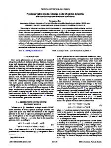
Figure 6. Snapshots of the system in time for different values of β = 0.0, 0.005, 0.1, and β → ∞ (top to bottom) showing that even for very small non-zero β, the system equilibrates towards a homogeneous state much faster compared to the β = 0 case. These snapshots are for a L = 100 system. Obviously, β → ∞ corresponds to Model I while letting β = 0 we have equal probabilities of the up and down states, making it equivalent to the zero temperature dynamics of the nearest neighbour Ising model. Since the equilibrium states for the extreme values β → ∞ and β = 0 are homogeneous (all up or all down states), it is expected that for all values of β they will remain so as is indeed the case.

It is useful to show the snapshots of the evolution of the system over time for different β (Fig.6): to be noted is the fact that for any non-zero β however small, the system equilibrates very fast compared to the Ising limit β = 0. The detailed dynamical studies in fact showed that the system belongs to the Model I dynamical class for any finite β and a dynamic transition takes place exactly at β = 0. Certain subtleties in this model need to be mentioned: with respect to Model I, β = 0 is the maximum noise and its inverse may be thought of an effective temperature. On the other hand, from the Ising model viewpoint, β plays the role of noise. However it is not equivalent to thermal fluctuations which can affect the state of any spin. With β, flipping of spins can still occur at the domain boundaries only. Hence, even with this noise, the equilibrium behaviour is not disturbed for any value of β (even for β → ∞ which corresponds to Model I) while in contrast, any non-zero temperature can destroy the order of a one dimensional Ising model. 2.2.3. Model with random cutoffs : Previously we have discussed the case when a uniform cutoff is introduced to the system. One can introduce randomness in the cutoff parameter p varying from 0 to 1, (chosen randomly from a uniform distribution) and associated with each individual a different value of p [17]. The randomness is quenched as the value of p assumed by any individual is fixed for all times. In this case, the variation of the magnetization, domain walls and persistence show power law scalings with exponents corresponding to Model I only for an initial range of time; however, calculation of z from the saturation times gives z = 1. The later time behaviour appears to deviate from the Model I behaviour and further studies are required to analyses the exact dynamical behaviour. 140

80

70

120

60 100

Time

Time

50 80

60

40

30 40 20 20

10

0

0 0

10

20

30

40

50

Sites

(a)

60

70

80

90

100

0

10

20

30

40

50

60

70

80

90

100

Sites

(b)

Figure 7. Snapshots of the system in time for (a) random cutoff parameter p varying from 0 to 1, and (b) uniform cutoff parameter p. These snapshots are for a L = 100 system.

Even snapshots of the system (when compared to the uniform cutoff or infinite cutoff cases) do not help in understanding the phenomenon much (Fig 7). 3. Mapping of the opinion dynamics model to reaction diffusion system The opinion dynamics model discussed so far are models where the dynamics is described in terms of the Ising spins that mimic the binary opinions an individual can have. In this model, a spin deep inside a domain does not flip. The dynamics is governed by the flipping of the spins only at the domain walls. The dynamics, in this respect, is reminiscent of the zero temperature Glauber dynamics of the kinetic Ising model. The motions of the domain walls can be viewed as the motions of the particles A with the reaction A+ A → ∅. This means the particles are walkers

and when two particles come on top of each other they are annihilated. The annihilation reaction ensures domain coalescence and coarsening. Unlike that in Glauber Ising model, the walkers A corresponding to Model I do not perform random walks. These walkers move ballistically towards their nearest neighbours. This bias, as we have seen before, gives rise to a new universality class than that of conventional reaction diffusion system [20]. We have also studied A + A → ∅ model with the particles A performing random walk with a bias ǫ towards their nearest neighbors. We have taken ǫ as the probability that a walker walks towards its nearest neighbour. Clearly, ǫ = 0.5 corresponds to usual reaction diffusion system with the particles performing random walk. On the other hand, ǫ = 1 is equivalent to our Model I as has been described above. We have studied the dynamics of the reaction diffusion system for different values of ǫ in the range [0+ , 1.0]. In reaction diffusion systems, the growth of domains is given by the number of surviving walkers. Persistence P (t) in these systems is defined as the fraction of sites unvisited by any of the walkers A till time t. Figures 8 and 9 show the decay of persistence and fraction of walkers with time for different values of ǫ > 0.5. 1 L=500,ε=0.7 L=1000,ε=0.7 L=1000,ε=0.55 L=500,ε=0.55 slope=-0.23

0.7

Persistence

0.5 0.3

0.1

100

101

102

103

104

105

Time

Figure 8. Decay of persistence with time for ǫ = 0.7 and ǫ = 0.55

We find that for ǫ > 0.5, the Model I behaviour is observed, namely: z ≃ 1.0 and θ ≃ 0.235, with some possible correction to the scaling which becomes weaker as ǫ is increased. For example, there is a logarithmic correction to scaling for the decay of the fraction of domain walls which takes the form t−1 (1 + α(ǫ) log(t)) where α(ǫ) → 0 as ǫ → 1. One can compare the above model with the cases discussed in section 2.2.3, where the introduction of stochastic dynamics also occurred with a bias towards the larger domain. In case of thermal disorder, the parameter comparable to ǫ is β. In the present case, the exact sizes of the domains do not matter (which is important for the case with β) but the results are consistent in the sense that any bias towards the larger domain (or nearest walker) makes the system behave like Model I. In this model, we have also studied the ǫ < 0.5 region where the opposite happens, the walker has a bias towards the further neighbour. Obviously domain annihilations take place very slowly now, even slower than 1/ log(t) and the dynamics continues for very long times. Consequently, the persistence probability no longer shows a power law variation now but falls exponentially to zero (Fig 10).

Fraction of walkers

100

L=500,ε=0.7 L=1000,ε=0.7 L=1000,ε=0.55 L=500,ε=0.55 slope=-1.0 f(t)

10-1

10-2

10-3

100

101

102

103

104

105

Time

Figure 9. Decay of number of walkers with time for ǫ = 0.7 and ǫ = 0.55. There is a logarithmic correction to scaling for the value of ǫ = 0.55. The form of f (t) is t−1 (1 + α log(t)) with α = 3.92 100

Dw(t)*0.4,ε=0.3 Dw(t)*0.4,ε=0.45 P(t),ε=0.45 P(t),ε=0.3 g(t)

10-1

10-2

10-3

10-4 100

101

102

103

104

105

Time

Figure 10. Decay of persistence and number of walkers with time for ǫ = 0.3 and ǫ = 0.45. The form of g(t) is a(1/ log(t)) where a is any constant.

4. Summary and Discussions We have reviewed the dynamics of a recently proposed opinion dynamics model (Model I and its variations) [8]. Model I in one dimension belongs to a new dynamical universality class with novel dynamical features not encountered in any previous models of dynamic spin system or opinion dynamics. In the corresponding reaction diffusion system A + A → ∅, we have introduced a probability ǫ of random walkers A moving towards their nearest neighbors. ǫ = 0.5 corresponds to the particles A performing unbiased random walks and the system belongs to the dynamical universality class of zero temperature Glauber Ising model. We find that for ǫ > 0.5, the system still shows power law behavior of domain growth and persistence but with a universality class of that of Model I. For ǫ < 0.5, the domain grows logarithmically and the persistence decays exponentially in time. We have discussed quite a few variations on Model I with quenched and annealed disorders

and cutoffs in the interaction range. In presence of quenched disorders, like the presence of few rigid spins which do not flip, the dynamics changes drastically. The dynamics ends up in heterogeneous equilibrium phases, which is fully disordered in the sense that no consensus can be reached as the order parameter goes to zero in the thermodynamic limit, with identical behaviour irrespective of the percentage of the rigid spins in the system. However, the dynamics shows extreme robustness against annealed disorder. We have also discussed the crossover phenomena in the dynamics in presence of cutoffs in the range over which a spin recognizes its neighboring domains. All the models discussed in the present article can easily be extended to higher dimensions and its universality class determined. Phase transitions occurring at non-extreme values of suitably defined parameters may also be expected in higher dimensions. Acknowledgements: SB and PS acknowledge financial support from DST project SR/S2/CMP-56/2007. Partial computational help has been provided by UPE project. SB acknowledges the hospitality of IMSc where part of the work was done. PR acknowledges the Department of Physics, University of Calcutta for hospitality. References [1] Econophysics and Sociophysics: Trends and Perspectives, Eds. Chakrabarti B K, Chakrabarti A and Chatterjee A, Wiley VCH, Berlin (2006). [2] Castellano C, Fortunato S and Loreto V (2009) Rev. Mod. Phys. 81 591. [3] Schelling T C (1971) J. Math. Sociol. 1: 143 [4] Stauffer D, in Encyclopedia of Complexity and Systems Science edited by Meyers R A (Springer, New York, 2009); [5] Baronchelli A, Dall’Asta L, Barrat A, and Loreto V, Phys. Rev. E 76, 051102 (2007); Castellano C, Marsili M and Vespignani A, Phys. Rev. Lett. 85 3536 (2000). [6] Liggett T M Interacting Particle Systems: Contact, Voter and Exclusion Processes (Springer-Verlag Berlin 1999). [7] Sznajd-Weron K and Sznajd J, Int.J.Mod.Phys C 11 1157 (2000). [8] Biswas S and Sen P, Phys. Rev. E 80, 027101 (2009). [9] Castellano C, Vilone D and Vespignani A, Europhys. Lett. 63 153 (2003). [10] Derrida B, Bray A J and Godreche C, J.Phys. A 27 L357 (1994). [11] Manoj G and Ray P, Phys. Rev. E 62 7755 (2000); Manoj G and Ray P, J. Phys A 33 5489 (2000). [12] Biswas S, Chandra A K and Sen P, Phys. Rev. E 78, 041119 (2008) [13] Derrida B in Lecture notes in Physics 461 165 (Springer, 1995); Derrida B, Hakim V, Pasquier V, Phys. Rev. Lett. 75 751 (1995) [14] Stauffer D and de Oliveira P M C, Eur. Phys. J B 30 587 (2002.) [15] Sanchez J R, arXiv:cond-mat/0408518v1 [16] Shukla P, J. Phys. A Math. Gen. 38 5441 (2005). [17] Biswas S and Sen P, Journal of Physics A 44 145003 (2011). [18] Galam S, Physica A 381 366 (2007) [19] Sen P, Phys. Rev. E 81, 032103 (2010) [20] Redner S, in Nonequilibrium Statistical Mechanics in One Dimension edited by Privman V (Cambridge University Press, Cambridge, 1997)