call this joint time-slot and power allocation power scheduling. As pointed out in ...... We assume that the base-station is located at the center of the cell and that ...
Opportunistic Power Scheduling for Multi-server Wireless Systems with Minimum Performance Constraints Jang-Won Lee, Ravi R. Mazumdar, and Ness B. Shroff School of Electrical and Computer Engineering Purdue University West Lafayette, IN 47907, USA {lee46, mazum, shroff}@ecn.purdue.edu
Abstract— In this paper, we present a power scheduling scheme, i.e., a joint time-slot and power allocation method for wireless cellular systems. We allow multiple transmissions in a timeslot that can interfere with each other. Hence, it is important to not only select the mobiles to be scheduled in a time-slot, but also important to allocate an appropriate power level for transmission to these scheduled mobiles in order to achieve high system performance and quality of service. We model the timevarying wireless channel as a stochastic process and formulate a stochastic programming problem that attempts to maximize the expected total system utility, with constraints on the minimum expected utility for each mobile. The power scheduling algorithm is obtained by using stochastic duality and implemented via stochastic subgradient techniques.
I. I NTRODUCTION The continued increase in demand for wireless services as well as the scarcity of radio resources makes it imperative to efficiently utilize network resources and achieve high system performance. A unique characteristic of wireless systems is that, due to fading and mobility, the wireless channel is timevarying and location-dependent. Although at first this appears to be a drawback, one can actually exploit the variations in the channel condition to improve network performance [1], [2], [3], [4]. It is well known that by giving a higher transmission priority to a mobile experiencing a better channel condition (e.g., a mobile that is closer to a base-station), one can increase the system throughput. However, as pointed out in [1], [2], [3], this naive strategy results in unfair resource allocation, thus potentially violating the performance or Quality of Service (QoS) requirements of some mobiles. Hence, one has to carefully consider the trade-off between system efficiency and fairness among mobiles when scheduling mobiles in wireless networks. Recently, various “opportunistic” scheduling schemes have been developed for wireless networks (see [1], [2], [3], [4], [5], [6], [7], [8] and references therein). These schemes exploit the characteristics of the changing wireless channel and at the same time provide certain fairness or performance guarantees. This research has been supported in part by NSF grants ANI-0073359, ANI-9805441, and ANI-0207728.
0-7803-8356-7/04/$20.00 (C) 2004 IEEE
We can classify these scheduling schemes as either “singleserver” scheduling or “multi-server” scheduling based on the underlying multiple access scheme used. In “single-server” scheduling, only one mobile is served at a time (e.g., a Time Division Multiple Access (TDMA) type of the multiple access scheme is used). For this class of scheduling schemes, a fixed power level is allocated to the scheduled mobile in the current time-slot in general. Hence, one only has to consider time-slot allocation without taking into account power allocation among mobiles. In contrast to “single-server” scheduling, in “multi-server” scheduling, multiple mobiles can be served simultaneously (e.g., a Code Division Multiple Access (CDMA) type of the multiple access scheme is used to allow simultaneous user transmissions). For this class of scheduling schemes, the transmission power of simultaneously scheduled mobiles could, in general, interfere with each other. Hence, one must simultaneously consider the problems of power allocating power as well as time-slot among the scheduled mobiles. Since the procedure to allocate time-slots is equivalent to allocating zero power to unscheduled mobiles and positive power to the scheduled mobiles in the corresponding time-slot, we simply call this joint time-slot and power allocation power scheduling. As pointed out in [7] and [8], in contrast to “singleserver” scheduling, there has been relatively little work on “multi-server” scheduling problems. However, “multi-server” transmission (e.g., CDMA) is adopted as a multiple-access scheme in third generation systems [9] and continues to be a strong candidate for future generation systems. Further, as shown in [10], a static TDMA type of multiple access scheme, i.e., “single-server” scheduling can be inefficient, since the optimal multiple access scheme depends on the dynamic system environment. Hence, it is quite important to develop an efficient power scheduling scheme for “multi-server” systems. In this paper, we will study the opportunistic power scheduling problem for “multi-server” wireless systems. Our work has similarity to works in [1], [2], [3], [5], [6] in the sense that they model the channel condition as a stochastic process and develop appropriate scheduling strategies. However, in these works only the mobile selection problem
IEEE INFOCOM 2004
is considered (i.e., which mobiles should be scheduled to transmit in a given time-slot) without considering the power that should be allocated to each mobile (the reason is that only a single mobile can be selected for transmission at a time in [1], [2], [3], [6] and mobiles that are selected for transmission are assumed to communicate using independent interfaces with each other in [5]). Our work also has similarity to the work in [4]. In [4], a scheduling problem that attempts to maximize the total expected throughput with constraints on fairness and on the maximum total transmission power is studied. In this work, since multiple mobiles can be scheduled in a time-slot and the maximum total transmission power is also constrained, both mobile selection and power allocation problems are considered. However, in [4], each link is assumed to be orthogonal and not to interfere with each other. Further, it is assumed that there is a linear relationship between the scheduled rate and the power consumed. These assumptions are not required in our work. Moreover, we consider a problem with constraints on minimum performance for each mobile, which is different from the fairness constraints in [4]. Hence, the algorithm developed in [4] is not applicable to our problem. The paper is organized as follows. In Section II, we introduce the system model. In Section III, we present our scheduling algorithm. In Section IV, we discuss some implementation issues. We provide numerical results in Section V and conclude in Section VI.
P¯s :
Power allocation vector for all mobiles when the system is in state s. Ps,i : Power allocation for mobile i when the system is in state s. Ni : A constant for mobile i. Gs,i : Path gain from the base-station to mobile i when the system is in state s. Is,i : Background noise and intercell interference at mobile i when the system is in state s. θ: Orthogonality factor. M : Number of mobiles in the cell. In this equation, if Ni = 1, then the signal quality metric γs,i represents the signal to interference and noise ratio (SINR) for mobile i. If Ni is the processing gain for mobile i, which is defined by W/Ri , where W is the chip rate and Ri is the data rate, then γs,i represents the bit energy to interference density ratio of mobile i, (Eb /I0 )s,i in the CDMA system, and if Ni = W , then γs,i = (Eb /I0 )s,i Ri of mobile i in the CDMA system. We assume that the utility function, Ui , has the following properties that cover most practical types of utility functions for wireless systems. (A1) (A2) (A3) (A4)
II. S YSTEM M ODEL We focus on the downlink of a cell that consists of a single base-station and M mobiles. We assume that the wireless system is time-slotted. A time-slot in our system is an arbitrary interval of time and could consist of one packet or several packets. In each time-slot, mobiles are selected for transmission and the transmission power for each selected mobile is determined. The base-station has a maximum transmission power limit, PT . In wireless systems, interference, background noise, and path gain are time-varying and they can be modeled as stochastic processes. We assume that they are fixed during a time-slot. However, we allow that they vary across timeslots and model them as stationary stochastic processes. In a time-slot, the system is assumed to be in one of several possible states, in which each state represents one of several possible levels of interference, background noise and path gain for all mobiles. Each state takes a value from a finite set {1, 2, · · · , S}1 . We denote the probability that the system is in state s as πs . We first define the “generic” signal quality for mobile i when the system is in state s: γs,i (P¯s )
=
Ni Gs,i Ps,i , �M θGs,i ( j=1 Ps,j − Ps,i ) + Is,i
(1)
where 1 Note
that this assumption is not so restrictive, since in a real system interference and path gain are mapped into a level set with a finite number of levels by using quantization.
0-7803-8356-7/04/$20.00 (C) 2004 IEEE
Ui is an increasing and continuous function of γs,i . Ui (0) = 0. is bounded above. Ui � M If j=1 Ps,j = PT , then Ui (γs,i (Ps,i )) is one of three types: a sigmoidal-like 2 , a strictly concave, or a strictly convex function of its own power allocation, Ps,i .
III. O PPORTUNISTIC P OWER S CHEDULING WITH THE M INIMUM P ERFORMANCE C ONSTRAINT In this section, we study a power scheduling problem that attempts to maximize the expected total system utility with constraints on the maximum transmission power limit of the base-station, PT , and the minimum expected utility for each mobile i, Ci . Then, the optimization problem is formulated as: (A)
max
S �
πs
s=1
s. t.
S � s=1 M � i=1
M �
Us,i (Ps,i )
i=1
πs Us,i (Ps,i ) ≥ Ci , i = 1, 2, · · · , M, Ps,i ≤ PT ,
0 ≤ Ps,i ≤ PT ,
s = 1, 2, · · · , S, s = 1, 2, · · · , S, i = 1, 2, · · · , M,
�
where Us,i (Ps,i )= Ui (γs,i (Ps,i )) and by using a simple observation that to maximize the total system utility, the base-station sigmoidal-like function means a function fi (x) that has one inflection d2 f (x) d2 f (x) point, xo and dxi 2 > 0 for x < xo and dxi 2 < 0 for x > xo , i.e., fi (x) is strictly convex for x < xo and strictly concave for x > xo . 2A
IEEE INFOCOM 2004
always has�to transmit at its maximum transmission power M limit, i.e., i=1 Ps,i = PT [11], [12], we redefine γs,i (P¯s ) in (1) as Ni Gs,i Ps,i � . γs,i (Ps,i )= θGs,i (PT − Ps,i ) + Is,i �M Remark 1: Since i=1 Ps,i = PT , by (A4), Us,i (Ps,i ) is one of three types: a sigmoidal-like, a strictly concave, or a strictly convex function of Ps,i . The above can be formulated as a stochastic programming problem [13], [14]. We assume that there exists at least one interior feasible solution in the above problem. Then, the first question that arises before solving this problem, is how to ensure feasibility, i.e., how do we ensure that there exists a scheduling policy that satisfies the constraints. This can be achieved by adopting an appropriate call admission control strategy. In this paper, we assume that the system has a call admission control policy in place that ensures the feasibility of the problem and focus on the scheduling problem. Note that if instead of an absolute QoS constraint on the utility received by each user, if we used a relative constraint (either in terms of time-slots or utility), as in [3], then there would be no issue of infeasibility. In solving problem (A), there exist two main difficulties: one is that since we allow non-concave utility functions, problem (A) may not be a convex programming problem (note that, in general, the utility function in wireless networks need not be formulated as concave functions [10], [11], [12], [15], [16], [17]). The other is that, in practice, we do not have information for the state of the system a priori, i.e., we do not have knowledge of the underlying probability space. Hence, the main effort in this paper will be devoted to overcome these two difficulties. To deal with the non-convexity of the problem, we consider the dual of problem (A). The dual is always a convex programming problem and, thus, it has more structure than the primal problem (A). We first define a Lagrangian function associated with problem (A). � To that end, we use that the M constraint on the power limit, i=1 Ps,i ≤ PT is equivalent �M to πs i=1 Ps,i ≤ πs PT . Then, the Lagrangian function, ¯ P¯ ) is defined by Lmp (¯ µ, λ, ¯ P¯ ) µ, λ, Lmp (¯ S S M M � � � � πs Us,i (Ps,i ) + λs πs (PT − Ps,i ) = s=1 i=1 M S � �
+
µi (
i=1
=
S �
s=1 i=1 M �
mp Us,i (¯ µ, Ps,i ) + λs (PT −
i=1
M �
Ps,i ))
i=1
µi Ci ,
µ ¯ ≥¯ 0
where F mp (¯ µ)
= = =
¯ P¯ ) min max Lmp (¯ µ, λ, ¯ ¯ λ≥ 0 P¯ ∈Y
S �
πs min max Lmp µ, λs , P¯s ) − s (¯ λs ≥0 P¯s ∈Ys
s=1 S �
πs min
λs ≥0
s=1
Lmp µ, λs , P¯s ) s (¯
M �
=
M � i=1
µi Ci
i=1
Qmp µ, λs ) s (¯
−
M �
µi Ci ,
(2)
i=1
mp Us,i (¯ µ, Ps,i ) + λs (PT −
M �
Ps,i ),
i=1
Qmp µ, λs ) = max Lmp µ, λs , P¯s ), s (¯ s (¯ P¯s ∈Ys
¯0 = (0, 0, · · · , 0), Ys = {P¯s | 0 ≤ Ps,i ≤ PT , i = 1, 2, · · · , M }, and Y = {P¯ | P¯s ∈ Ys , s = 1, 2, · · · , S}. We now consider the problem in (2) for a given µ ¯. Since ¯ µ) = (λ1 (¯ µ), λ2 (¯ µ), · · · , λS (¯ µ)) solves it is separable in s, λ(¯ (2), if and only if λs (¯ µ) = arg min Qmp µ, λs ), s = 1, 2, · · · , S. s (¯ λs ≥0
(3)
Note that for a given system state s, the above problem is deterministic and we can solve it without knowledge µ, λs , P¯s ) of the underlying probability space. Since Lmp s (¯ µ, λs ) = is separable in i, for given µ ¯ and λs , P¯smp (¯ mp mp mp (¯ µ, λs ), Ps,2 (¯ µ, λs ), · · · , Ps,M (¯ µ, λs )) maximizes it, if (Ps,1 and only if mp Ps,i (¯ µ, λs ) =
arg
max
0≤Ps,i ≤PT
mp {Us,i (¯ µ, Ps,i ) − λs Ps,i },
i = 1, 2, · · · , M.
(4)
To solve the problem in (3), we first define λmax µ)=min{λ ≥ 0 | s,i (¯
mp max {Us,i (¯ µ, Ps,i ) − λs Ps,i }
0≤P ≤PT
= 0}, i = 1, 2, · · · , M, s = 1, 2, · · · , S.
� is a solution of the following equation: where Ps,i
i=1 mp where Us,i (¯ µ, Ps,i ) (P¯1 , P¯2 , · · · , P¯S ), P¯s
min F mp (¯ µ)
(B)
Then, from [11], [12], it can be shown that mp ∂Us,i (¯ µ,Ps,i ) |Ps,i =0 , ∂Ps,i mp if Us,i is a concave function mp ∂Us,i (¯ µ,Ps,i ) � , |Ps,i =Ps,i ∂P s,i mp λmax µ) = s,i (¯ is a sigmoidal-like function , if U s,i � exists and P s,i mp Us,i (¯ µ,PT ) , PT otherwise
πs Us,i (Ps,i ) − Ci )
s=1 M �
πs (
−
s=1
¯ = (λ1 , λ2 , · · · , λS ). Then, the dual (µ1 , µ2 , · · · , µM ), and λ of problem (A) is defined as:
= =
(1 + µi )Us,i (Ps,i ), P¯ (Ps,1 , Ps,2 , · · · , Ps,M ), µ ¯
0-7803-8356-7/04/$20.00 (C) 2004 IEEE
= =
mp (¯ µ, Ps,i )−Ps,i Us,i
mp ∂Us,i (¯ µ, Ps,i ) o = 0, Ps,i (¯ µ) ≤ Ps,i ≤ PT ∂Ps,i
IEEE INFOCOM 2004
mp o and Ps,i (¯ µ) is an inflection point of Us,i (¯ µ, Ps,i ) when µ ¯ is mp (¯ µ, λs ) has the fixed. We can show that, for a given µ ¯, Ps,i following properties [11], [12]:
(P1) (P2)
(P3)
mp (¯ µ, λs ) Ps,i mp Ps,i (¯ µ, λs )
is non-increasing in λs . is discontinuous and has two valµ) when ues (zero and positive) at λs = λmax i,s (¯ mp (¯ µ, Ps,i ) is a sigmoidal-like or convex function. Us,i Otherwise, it is continuous and has a unique value. mp (¯ µ, Ps,i ) is a sigmoidal-like function and If Us,i mp mp o µ, λs ) > 0, then Ps,i (¯ µ, λs ) ≥ Ps,i (¯ µ), where Ps,i (¯ mp o µ) is an inflection point of Us,i (¯ µ, Ps,i ). Ps,i (¯
mp (¯ µ, λs ) = Ps,i �� ≤ Ps,i (¯ µ, λs ).
In the following, we assume that � �� � (¯ µ, λs ), Ps,i (¯ µ, λs )} and Ps,i (¯ µ, λs ) {Ps,i mp µ, Ps,i ) is a sigmoidal-like or convex function Hence, if Us,i (¯ � �� µ), then 0 = Ps,i (¯ µ, λs ) < Ps,i (¯ µ, λs ). and λs = λmax i,s (¯ � �� µ, λs ) = Ps,i (¯ µ, λs ). Otherwise, Ps,i (¯ By Danskin’s Theorem [18], the subdifferential of µ, λs ), ∂λs Qmp µ, λs ) with respect to λs is obtained Qmp s (¯ s (¯ as:
∂λs Qmp µ, λs ) = s (¯ M M � � �� � Ps,i (¯ µ, λs ) ≤ d ≤ PT − Ps,i (¯ µ, λs )}.(5) {d | PT − Since we can easily show that λs (¯ µ) �= 0, from the theory of the subdifferential [18], it solves the problem in (3), if and only if (6)
mp In this case, Ps,i (¯ µ, λs (¯ µ)), i = 1, 2, · · · , M can be the corresponding primal solution (i.e., power allocation for given system state s and µ ¯). However, note that when the subgradient µ, λs ) is not unique at λs (¯ µ), we have multiple of Qmp s (¯ � primal solutions (power allocation), i.e., Ps,i (¯ µ, λs (¯ µ)) < �� µ, λs (¯ µ)) for some mobile i and some choices among Ps,i (¯ them result in infeasible power allocation (i.e., the sum of power allocation for each mobile can exceed PT , the maximum transmission power limit). Hence, in the following, we develop an algorithm that chooses a feasible primal solution (in terms of the maximum transmission power limit). We assume that system state s and µ ¯ are given and mobiles µ), i.e., λmax µ) ≥ are ordered in a decreasing order of λmax s,1 (¯ s,i (¯ max max 3 λs,2 (¯ µ) ≥ · · · ≥ λs,M (¯ µ) . If multiple mobiles have the µ), they are ordered randomly. We first select same λmax s,i (¯
order of mobiles can differ for different system state s or µ ¯.
0-7803-8356-7/04/$20.00 (C) 2004 IEEE
�� Ps,i (¯ µ, λmax µ)) ≤ PT }. s,j (¯
i=1
(7) Hence, mobiles are selected in a decreasing order of λmax (¯ µ ). s,i If Ks (¯ µ)
�
�� Ps,i (¯ µ, λmax µ)) < PT and s,Ks (¯ µ)+1 (¯
i=1 Ks (¯ µ)+1
� i=1
�� Ps,i (¯ µ, λmax µ)) > PT , Ks (¯ µ) < M, (8) s,Ks (¯ µ)+1 (¯
mp µ) = λmax µ, λmax then λs (¯ s,Ks (¯ s,Ks (¯ µ)+1 , since 0 ∈ ∂λs Qs (¯ µ)+1 ). ∗ µ) such that Otherwise, we can find a λs (¯ Ks (¯ µ)
�
M �
�� Ps,i (¯ µ, λ∗s (¯ µ)) +
i=1
� Ps,i (¯ µ, λ∗s (¯ µ))
i=Ks (¯ µ)+1
Ks (¯ µ)
�
�� Ps,i (¯ µ, λ∗s (¯ µ)) = PT .
(9)
µ, λ∗s (¯ µ)), λs (¯ µ) = λ∗s (¯ µ). In this case, since 0 ∈ ∂λs Qmp s (¯ µ) = Hence, we can obtain the desired primal solution P¯s∗ (¯ ∗ ∗ ∗ (¯ µ), Ps,2 (¯ µ), · · · , Ps,M (¯ µ)) as (Ps,1 � �� µ, λs (¯ µ)), if i ≤ Ks (¯ µ) Ps,i (¯ ∗ (¯ µ) = , (10) Ps,i � Ps,i (¯ µ, λs (¯ µ)), otherwise where
� λs (¯ µ) =
i=1
µ, λs (¯ µ)). 0 ∈ ∂λs Qmp s (¯
j �
i=1
where P¯smp (¯ µ, λs ) is a set of solutions of the problem in (4) at µ ¯ and λs , and conv(G) is a convex hull of a set G. Hence, µ, λs ) at λs as: we can obtain ∂λs Qmp s (¯
3 The
µ) = max{1 ≤ j ≤ M | Ks (¯
=
µ, λs ) ∂λs Qmp s (¯ ∂Lmp (¯ µ, λs , P¯s ) ¯ =conv({ s | Ps ∈ P¯smp (¯ µ, λs )}), ∂λs
i=1
mobiles from 1 to Ks (¯ µ) that satisfy
λmax s,Ks (¯ µ)+1 , if (8) is satisfied λ∗s (¯ µ), otherwise
and λ∗s (¯ µ) is a solution of (9). Thus far, we have solved the problem in (3) for given system state s and µ ¯. We now solve problem (B). Note that F mp (¯ µ) is a convex function of µ ¯ and, thus, problem (B) is a stochastic µ) convex programming problem. However, to minimize F mp (¯ over µ ¯ ≥ ¯0, we need knowledge of the underlying probability space, i.e., πs , s = 1, 2, · · · , S, which is infeasible in practice. Hence, we will use a stochastic subgradient method [14], [19]. This is defined by the following iterative process: (n+1)
µi
=
(n)
[µi
(n)
− α(n) vi ]+ , i = 1, 2, · · · , M, (11) (n)
where [a]+ = max{0, a} and vi is a random variable. Let ¯(1) , · · · , µ ¯(n) be generated by the sequence of solutions µ ¯(0) , µ (n) (n) (n) (n) (11) and v¯ = (v1 , v2 , · · · , vM ) be chosen such that ¯(0) , µ(1) , · · · , µ(n) } ∈ ∂µ¯ F mp (¯ µ(n) ), E{¯ v (n) | µ where ∂µ¯ F mp (¯ µ(n) ) is the subdifferential of F mp (¯ µ(n) ) with (n) (n) is called respect to µ ¯ at µ ¯ = µ ¯ . Then, the vector v¯ a stochastic subgradient. In this case, by solving (11), µ ¯(n) o converges to µ ¯ , the optimal solution of problem (B), with probability 1, if the following conditions are satisfied: ¯(0) , µ(1) , · · · , µ(n) } ≤ c E{||¯ v (n) ||2 | µ
(12)
IEEE INFOCOM 2004
for a constant c and ∞ ∞ � � α(n) = ∞, and (α(n) )2 < ∞. α(n) ≥ 0, n=0
(13)
n=0
µ) is obtained by By Danskin’s Theorem [18], ∂µ¯ F mp (¯ ∂µ¯ F mp (¯ µ) = {(d1 , d2 , · · · , dM ) |
S �
� πs Us,i (Ps,i (¯ µ, λs (¯ µ))) − Ci
s=1
≤ di ≤
S �
�� πs Us,i (Ps,i (¯ µ, λs (¯ µ))) − Ci , ∀i}.
(14)
s=1
Hence, if we let gimp (¯ µ(n) )
=
S �
∗ πs Us,i (Ps,i (¯ µ(n) )) − Ci , i = 1, 2, · · · , M,
s=1
∗ where Ps,i (¯ µ(n) ) is defined in (10), then mp (n) (g1mp (¯ µ(n) ), g2mp (¯ µ(n) ), · · · , gM (¯ µ )) ∈ ∂µ¯ F mp (¯ µ(n) ).
This implies that if we take (n)
vi
= Us(n) ,i (Ps∗(n) ,i (¯ µ(n) )) − Ci , i = 1, 2, · · · , M,
(15)
where s(n) is an index of the system state at iteration n, the algorithm in (11) converges to the optimal solution that solves problem (B) with a sequence of step sizes that satisfies conditions given in (13). Thus far, we have shown that the dual of problem (A) can be solved by using a stochastic subgradient method even without knowledge of the underlying probability space. If problem (A) is a stochastic convex programming problem, (i.e., Us,i (Ps,i ), ∀i, ∀s is a concave function), there is no duality gap between it and its dual. Hence, we can obtain its optimal power scheduling by solving its dual [13]. However, since problem (A) may not be a stochastic convex programming problem, typically, we can guarantee neither optimality, nor feasibility (in terms of minimum performance constraints4 ) of the solution that is obtained by solving the dual. Hence, in the following, we study the optimality and the feasibility of our power scheduling method, and show that an increase in the number of mobiles and the randomness of the system can improve the degree of the feasibility and optimality of our solution. ¯ o be the optimal dual solutions, and P ∗ (= Let µ ¯o and λ s,i ∗ o o µ )) and Ps,i , s = 1, 2, · · · , S, i = 1, 2, · · · , M be the Ps,i (¯ power allocations for our power scheduling method and the global optimal power scheduling, respectively. Define a subset of mobiles Qs as Qs
mp o = {1 ≤ i ≤ M | λmax µo ) = λos and Us,i (¯ µ , Ps,i ) s,i (¯ is a non-concave function}, s = 1, 2, · · · , S (16)
|Qs | as its cardinality, and a set Zi for mobile i as Zi = {1 ≤ s ≤ S | i ∈ Qs }, i = 1, 2, · · · , M. 4 Note
that the way in which we choose a primal solution in (10), our power scheduling is always feasible in terms of the total transmission power limit.
0-7803-8356-7/04/$20.00 (C) 2004 IEEE
The next two propositions show the asymptotic feasibility (in terms of minimum performance constraints) of our power scheduling. � S
1: If �Proposition �S
πs |Qs | M
s=1
∗ πs Us,i (Ps,i )−Ci
→ 0 as M → ∞, then
→ 0 as M → ∞, where H = M � S ∗ π U (P {1 ≤ i ≤ M | s s,i s,i ) − Ci < 0}. s=1 Proof: See Appendix B The condition in Proposition 1 is satisfied when the expected µo ) in each timenumber of mobiles that have the same λmax s,i (¯ slot is small compared to the total number of mobiles. Since µo ) of each mobile i depends on Us,i , it depends on λmax s,i (¯ the channel conditions of mobile i such as Gs,i , path gain from the base-station to mobile i, and Is,i , background noise and intercell interference at mobile i. Hence, in general, each µo ) and the condition is satisfied mobile i has different λmax s,i (¯ in most cases. Proposition 1 implies that if there exist a large number of mobiles that achieve utilities that are less than their constraints, the difference between the constraint and the achieved utility of each of those mobiles would be small. On the other hand, it also implies that if some mobiles achieve utilities much less than their constraints, the number of those mobiles would be small compared with the total number of mobiles. �S ∗ Proposition 2: If � Zi = ∅, then s=1 πs Us,i (Ps,i ) ≥ Ci . Otherwise, if s∈Zi πs → 0 as S → ∞, then �S ∗ π U (P ) ≥ C s s,i i − � and � → 0 as S → ∞. s,i s=1 Proof: See Appendix C Proposition 2 implies that if the condition in the proposition is satisfied for each mobile, our power scheduling guarantees that asymptotically each individual mobile’s QoS constraints are met. This condition can be satisfied when there exist a large number of mobiles in the system and the probability of the event that a mobile belongs to one of sets Qs , s = 1, 2, · · · , S is small and well-distributed among the mobiles. The next proposition implies that our power scheduling is asymptotically optimal. �M �S o Proposition 3: If i=1 s=1 πs Us,i (Ps,i ) → ∞ and � i∈H
s=1
S
π |Q |
s s �M �s=1 → 0 as M → ∞, S o ) πs Us,i (Ps,i i=1� s=1� M S ∗ πs Us,i (Ps,i ) s=1 then �i=1 ≥ 1 − � and � → 0 as M → ∞. M �S o i=1
s=1
πs Us,i (Ps,i )
Proof: See Appendix D. Proposition 3 implies that our power scheduling can provide a higher system utility than the global optimal power scheduling. The reason for this is that our power scheduling may not be able to meet the constraints of problem (A) (in terms of minimum performance constraints). However, when our power scheduling meets the constrains (i.e., is feasible), by the definition of the global optimal power scheduling and Proposition 3, we have result. �S the following ∗ π U (P ) Corollary 1: If s s,i s,i − Ci ≥ 0, ∀i, and s=1 �M �S o π U (P ) → ∞ and s,i i=1� s=1 s s,i S
�M �s=1 S i=1
πs |Qs |
s=1
o ) πs Us,i (Ps,i
→
0 as M
→
∞, then
IEEE INFOCOM 2004
�M �S ∗ πs Us,i (Ps,i ) s=1 �i=1 → 1 as M → ∞. M �S o i=1
s=1
πs Us,i (Ps,i )
All the above results imply that if there exist a large number of mobiles and enough randomness in the system, a power scheduling obtained by solving the dual is quite close to the global optimal power scheduling, even though the primal is not a convex programming problem.
BS
BS
BS
BS
BS
BS
BS
BS
BS
IV. I MPLEMENTATION I SSUES To implement the opportunistic power scheduling scheme that has been developed in the previous section, each mobile needs to inform the base-station of its utility function when a call is initiated. In each time-slot, the base-station selects mobiles to be currently scheduled and determines the transmission power level for these mobiles in the following way. In time-slot n, each mobile measures its path gain and interference, and sends this information to the base-station. By using the measured data, the base-station calculates the power allocation vector in the time-slot by solving (7) and (10). Further, based on the achieved utility value in the current time-slot, the base-station adjusts µ ¯(n+1) for the next time-slot to find an appropriate weight factor, (1 + µoi ), for each mobile i by solving (11) and (15). Note that solving (7) and (10) in each time-slot n is equivalent to solving the dual of the following problem: (C)
max
M � i=1
(n)
(1 + µi )Us(n) ,i (Pi )
subject to
M �
Pi ≤ PT ,
i=1
0 ≤ Pi ≤ PT ,
i = 1, 2, · · · , M,
where s(n) is an index of the system state in time-slot n. Hence, we can infer that, in each time-slot, our opportunistic power scheduling method tries to solve problem (C) that maximizes the weighted sum of utility functions of all mobiles without minimum performance constraints. In this case, the minimum performance constraint of each mobile can be achieved by the appropriate weight factor. When the condition in (8) is satisfied, by solving (7) and (10), power is allocated to the selected mobiles (assuming µ) are selected) such that mobiles from 1 to Ks (¯ Ks (¯ µ)
�
�� Ps,i (¯ µ, λs (¯ µ)) < PT .
(17)
i=1
However, in this case, we can always find a λ∗s (¯ µ) such that Ks (¯ µ)
�
�� Ps,i (¯ µ, λ∗s (¯ µ)) = PT .
(18)
i=1 �� �� Since we can easily show that Ps,i (¯ µ, λs (¯ µ)) ≤ Ps,i (¯ µ, λ∗s (¯ µ)) for each selected mobile i, the power allocation in (18) provides the same utility or higher to each individual selected mobile than that in (17). Hence, we can slightly modify the power allocation algorithm in each time-slot to further increase
0-7803-8356-7/04/$20.00 (C) 2004 IEEE
Fig. 1.
Cellular network model.
the efficiency of the algorithm as follows: First, select mobiles µ) that satisfies (7) and, then, for the selected from 1 to Ks (¯ µ) that satisfies (18) and allocate power to mobiles, find a λ∗s (¯ �� (¯ µ, λ∗s (¯ µ)), i = 1, 2, · · · , Ks (¯ µ). the selected mobiles as Ps,i Note that this scheme is the same as the power allocation scheme that has been developed in [11], [12]. Hence, to determine power levels in each time-slot, we can use the power allocation scheme that has been developed in [11], [12]. V. N UMERICAL R ESULTS In this section, we provide numerical results to illustrate various features of our power scheduling scheme. We consider a CDMA system that consists of nine square cells, as in Fig. 1. We assume that the base-station is located at the center of the cell and that each base-station always transmits at its maximum transmission power limit, PT . We focus on the center cell of the system. We model path gain from the basestation to mobile i, Gs,i , as Gs,i
=
Ds,i , tα i
(19)
where ti is the distance from the base-station to mobile i, α is a distance loss exponent, and Ds,i is a log-normal distributed random variable with mean 0 and variance σ 2 (dB), which represents shadowing [20]. We let PT = 10, α = 4, and let the length of the side of the cell be 1000. We assume that mobile i has a sigmoid utility function that is expressed as Ui (γs,i ) = ci {
1 1+
eai (γs,i −bi )
− di },
ai bi
and di = 1+e1ai bi for normalization where we set ci = 1+e ea i b i (U (0) = 0 and U (∞) = 1). In the first experiment, we assume that there are 4 mobiles with the same utility function. We set ai = 0.5, bi = 7 dB, Ni = 32, and Ci = 0.59 for all mobiles, and σ = 4 dB. We assume that mobile i has a fixed distance ti = 100 × i from the base-station. Hence, mobile 1 is closest and mobile 4 is farthest from the base-station. In Fig. 2(a), we plot the trajectories of the average utility of each mobile. As shown in this figure, even though the minimum performance constraints
IEEE INFOCOM 2004
TABLE I C OMPARISON OF AVERAGE U TILITIES .
1 0.9
Mobile Non-opportunistic Our opportunistic Greedy
0.8 0.7
Utility
0.6
1 0.590 0.951 0.973
2 0.590 0.736 0.964
3 0.590 0.591 0.796
4 0.590 0.591 0.168
Total 2.360 2.869 2.901
0.5 0.4
4
0.3 0.2 0.1 0 0
2000
4000
6000
8000
10000
Slots
(a) Trajectories of the average utility of each mobile.
Ratio of average total system utilities
Opportunistic/Non−opportunistic Mobile 1 Mobile 2 Mobile 3 Mobile 4
3.5
3
2.5
2
1.5
0.9 Mobile 1 Mobile 2 Mobile 3 Mobile 4
0.8 0.7
1 1
Fig. 3.
0.6
2
3
4
5
σ
6
7
8
9
10
Ratios of average total system utilities.
µ
0.5 0.4 0.3 0.2 0.1 0 0
2000
4000
6000
8000
10000
Slots
(b) Trajectories of µ ¯(n) . Fig. 2.
Mobiles in different distance from the base-station.
for some mobiles may not be satisfied during the transient period, it is eventually satisfied for all mobiles. Also note that while the minimum performance constraints are satisfied for all mobiles, a higher average utility is given to a mobile that is closer to the base-station (i.e., a mobile that is experiencing a better channel condition), thus attempting to maximize average total system utility. We also plot the trajectories of µ ¯(n) in Fig. 2(b). The figure (n) shows that, µi ’s for mobiles that satisfy the performance constraint with equality (mobiles 3 and 4) converge to positive (n) values, while µi ’s for mobiles that satisfy the performance constraint with strict inequality (mobiles 1 and 2) converge to zero. The reason for this result can be explained as follows. As shown in the previous section, our algorithm is equivalent to solving the dual of problem (C) in each timeslot that attempts to maximize the weighted sum of all the mobiles’ utilities without minimum performance constraints, while minimum performance constraints are satisfied with an appropriate weight factor for each mobile. In this experiment, if each mobile has a unit weight factor (i.e., µi = 0 ∀i), the minimum performance constraint of mobile 4 cannot be satisfied (see greedy scheduling in Table I). Hence, to satisfy the minimum performance constraint of mobile 4, its weight factor (i.e., µ4 ) must be increased. By increasing the
0-7803-8356-7/04/$20.00 (C) 2004 IEEE
weight factor, more power can be scheduled to mobile 4, thus improving its performance. Further, since this causes a violation of the minimum performance constraint of mobile 3, its weight factor (i.e., µ3 ) is also increased. In this case, since mobile 4 is less efficient than mobile 3, mobile 4 needs a larger weight factor (i.e., a larger value of µi ) than that of mobile 3 to meet its performance constraint. However, for the efficiency of the system, the weight factors must be increased up to the values for which their minimum performance constraints are met with equality. On the other hand, the weight factors for the other mobiles that satisfy their minimum performance constraints with strict inequality are not increased, since the minimum performance constraints can be satisfied even without increasing the weight factors. We also compare the performance of our opportunistic power scheduling scheme with those of two other schemes. In the non-opportunistic scheduling scheme, in every timeslot, power is allocated to each mobile so that they achieve the same γs,i (however, the power allocation is done such that this is the maximum possible γs,i value). In the greedy power scheduling scheme, in every time-slot, power is allocated to each mobile so that the system utility of the time-slot can be maximized. This can be achieved by solving problem (C) with a unit weight factor for each mobile in every time(n) slot (i.e., µi = 0, ∀i, ∀n). However, since problem (C) is a non-convex programming problem, which is difficult to solve, we solve its dual for the greedy scheduling scheme. Hence, greedy scheduling is achieved by our opportunistic (n) scheduling scheme with µi = 0, ∀i, ∀n. We provide the average utility of each mobile and the average system utility for each scheduling scheme in Table I. For the simulation of our opportunistic power scheduling, we first simulate nonopportunistic power scheduling and take the achieved utility of each mobile in this scheduling as minimum performance constraints for our opportunistic scheduling. As this table
IEEE INFOCOM 2004
1 0.9
0.8
0.8
0.7
0.7
0.6
0.6 Utility
Utility
1 0.9
0.5
0.5
0.4
0.4
0.3
0.3
0.2
a1 = 0.5 a2 = 1.0
0.1 0 0
5
10 γ
15
Mobile 1 Mobile 2 Mobile 3 Mobile 4
0.2 0.1 0 0
20
2000
4000
6000
8000
(a) Sigmoid utility functions with different ai .
(a) Trajectories of the average utility of each mobile.
1
0.9 Mobile 1 Mobile 2 Mobile 3 Mobile 4
0.9
0.8 0.8
0.7
0.7
0.6
0.6
0.5
0.5
µ
Utility
10000
Slots
0.4
0.4
0.3
0.3
0.2
b =7 1 b2 = 9
0.1 0 0
5
10 γ
15
0.2 0.1 20
0 0
2000
4000
6000
8000
10000
Slots
(b) Sigmoid utility functions with different bi . Fig. 4.
Sigmoid utility functions.
shows, in the non-opportunistic power scheduling scheme, each mobile achieves the same average utility. However, since non-opportunistic scheduling does not exploit the channel condition, it results in the lowest total system utility. The greedy power scheduling scheme provides the highest total system utility, but it cannot satisfy the QoS constraint (e.g., it violates the minimum performance constraint for mobile 4). Compared with the other two schemes, our opportunistic power scheduling scheme satisfies the minimum performance of each user without significant loss in efficiency. In Fig. 3, we compare the performance of our opportunistic power scheduling and non-opportunistic power scheduling by varying the standard deviation σ of Ds,i in (19). A larger value of σ implies a larger fluctuation of path gain between the mobile and the base-station. As before, the minimum performance constraints for our opportunistic scheduling are determined based on the achieve utility of each mobile in non-opportunistic scheduling. The results show that as σ increases, the performance gain of our opportunistic power scheduling over non-opportunistic power scheduling increases. This implies that a larger fluctuation of path gain is of a larger advantage to our opportunistic power scheduling scheme, providing greater freedom to exploit the time-varying channel condition associated with each mobile. In the second experiment, we study the case when each
0-7803-8356-7/04/$20.00 (C) 2004 IEEE
(b) Trajectories of µ ¯(n) Fig. 5.
Mobiles with different ai .
mobile has a different utility function. We assume that all mobiles are at the same distance (ti = 250) from the basestation. Hence, on average, each mobile experiences the same channel condition. In Fig. 5, we set bi = 7 dB, Ni = 32, and Ci = 0.7 for all mobiles and ai = 1.0 − 0.1 × i for mobile i. Hence, if i < j, then ai > aj . As shown in Fig. 4(a), in the concave region, a sigmoid function with a larger value of ai needs a lower γs,i to achieve the same utility as a sigmoid function with a smaller value of ai . Hence, by (P3), it seems that a mobile with a larger value of ai utilizes power more efficiently than a mobile with a smaller value of ai . As shown in Fig. 5(a), in general, a mobile with a larger value of ai can achieve a higher utility than a mobile with a smaller value of ai . In this case, note that mobiles 1 and 2 get more than their minimum performance constraints, while mobiles 3 and 4 exactly meet their performance constraint (the equality constraints are met). Hence, as shown in Fig. 5(b), we have µoi = 0, i = 1, 2 and µo4 > µo3 > 0, because of the same reasons as for Fig. 2(b). In Fig. 6, we set ai = 0.5, Ni = 32, and Ci = 0.7 for all mobiles and bi = 3+2×i (dB) for mobile i. As shown in Fig. 4(b), a mobile with a smaller value of bi utilizes power more efficiently than a mobile with a larger value of bi . Therefore, as shown in Fig. 6(a), in general, a mobile with a smaller value of bi achieves a higher utility than a mobile with a larger value of
IEEE INFOCOM 2004
A PPENDIX
1
A. Properties of Dual and Primal Solutions
0.9 0.8 0.7
Utility
0.6 0.5 0.4 0.3 Mobile 1 Mobile 2 Mobile 3 Mobile 4
0.2 0.1 0 0
2000
4000
6000
8000
10000
Slots
(a) Trajectories of the average utility of each mobile.
1.4 Mobile 1 Mobile 2 Mobile 3 Mobile 4
1.2 1
µ
0.8 0.6 0.4 0.2 0 0
2000
4000
6000
8000
10000
Slots
(b) Trajectories of µ ¯(n) . Fig. 6.
Mobiles with different bi .
bi . In this figure, mobiles 2, 3, and 4 satisfy their performance constraints with equality. Hence, as shown in Fig. 6(b), we have µ1 = 0 and µ4 > µ3 > µ2 > 0 as explained before. VI. C ONCLUSION In this paper, we have developed an opportunistic power scheduling scheme for “multi-server” wireless systems in which each mobile has a minimum performance constraint. This scheme exploits the channel condition of each mobile and determines, in each time-slot, which, and how many mobiles, should be scheduled for transmission, and at what power levels. We have formulated the problem as a stochastic programming problem and solved it by using stochastic duality and a stochastic subgradient method. We have shown that the optimality and the ability of our power scheduling solution to meet all the QoS constraints are improved with an increase in the number of mobiles and the randomness of the system. The numerical results also show that as the variation of channel condition gets larger, the relative efficiency of our opportunistic power scheduling over non-opportunistic power scheduling increases. This implies that as the variation of channel condition gets larger, it becomes more important to exploit it appropriately.
0-7803-8356-7/04/$20.00 (C) 2004 IEEE
In this subsection, we study some properties of dual and primal solutions that are useful to prove the optimality and the feasibility of our power scheduling. Since we assume that there exists an interior feasible solution of the primal problem, by ¯o Proposition 3.2.3 in [21], there exist optimal dual solutions λ o ∗ � �� � �� and µ ¯ . We first let Ps,i and Ps,i = {Ps,i , Ps,i }, (Ps,i ≤ Ps,i ), s = 1, 2, · · · , S, i = 1, 2, · · · , M , be our power scheduling and primal solutions corresponding to optimal dual solutions ¯ o , respectively. Then, by (7) and (10), and properties µ ¯o and λ (P1) and (P2), � � �� , if i �∈ Qs Ps,i = Ps,i , ∀s, i, (20) � �� 0 = Ps,i < Ps,i , if i ∈ Qs � ∗ �� ≤ Ps,i ≤ Ps,i , ∀s, i. where Qs is defined in (16), and Ps,i � ∗ �� Hence, Us,i (Ps,i ) ≤ Us,i (Ps,i ) ≤ Us,i (Ps,i ), ∀s, i. �M �M � �� Lemma 1: PT − i=1 Ps,i ≥ 0 and PT − i=1 Ps,i ≤ 0, ∀s. Proof: This �S immediately�� follows from (5) and (6). Lemma 2: ≥ 0 and s=1 πs Us,i (Ps,i ) − Ci �S o � µi ( s=1 πs Us,i (Ps,i ) − Ci ) ≤ 0, ∀i. �S �� Proof: We first prove that s=1 πs Us,i (Ps,i ) − C �i S ≥ 0, ∀i. ��Suppose that there exists an i such that s=1 πs Us,i (Ps,i ) − Ci < 0. Then, by (14), the i th element µ) at µ ¯o is less than zero. This of each subgradient of F mp (¯ implies that if we take µ ¯ such that µi > µoi and µj = µoj , j �= i, d(¯ µ−µ ¯o ) < 0,
µ) at µ ¯o . However, since µ ¯o for each subgradient d of F mp (¯ mp is an optimal solution that minimizes F (¯ µ), by the theory of subdifferentials [18], there must exist a subgradient d of µ) at µ ¯o such that F mp (¯ d(¯ µ−µ ¯o ) ≥ 0, ∀¯ µ ≥ ¯0, �S �� which gives the contradiction. Hence, s=1 πs Us,i (Ps,i ) − Ci ≥ 0, ∀i. �S � We can prove that µoi ( s=1 πs Us,i (Ps,i ) − Ci ) ≤ 0, ∀i in a similar way � to the above case. �S M o �� Lemma 3: − Ci ) ≤ i( i=1 µ s=1 πs Us,i (Ps,i ) � S sups,i {µoi Us,i (PT )} s=1 πs |Qs |. Proof: From (20), M �
=
S � �� µoi ( πs Us,i (Ps,i ) − Ci )
s=1 i=1 M S � � � − µoi ( πs Us,i (Ps,i ) s=1 i=1 S � � �� πs µoi Us,i (Ps,i ) s=1 i∈Qs
≤ sup{µoi Us,i (PT )} s,i
S �
− Ci )
πs |Qs |.
s=1
IEEE INFOCOM 2004
Hence, by Lemma 2, 0 ≤
M �
S � �� µoi ( πs Us,i (Ps,i ) − Ci )
C. Proof of Proposition 2 � �� , Ps,i }, ∀s, i, as in Appendix A. We first define Ps,i = {Ps,i Then, from Lemma 2 and (20),
s=1
i=1
≤ sup{µoi Us,i (PT )} s,i
S �
πs |Qs |.
Ci
≤
S �
�� πs Us,i (Ps,i )
s=1
s=1
=
�
� πs Us,i (Ps,i )+
≤
� �� We first define Ps,i = {Ps,i , Ps,i }, ∀s, i, as in Appendix A. � ∗ Then, since Us,i (Ps,i ) ≤ Us,i (Ps,i ), ∀s, i, M � S � ∗ ( πs Us,i (Ps,i ) − Ci )
≥
i=1 s=1 M � S �
(
�
∗ πs Us,i (Ps,i )
S �
S �
≥
(
− Ci )
− sup{Us,i (PT )} s,i
S �
S �
πs |Qs |.
s=1
0 ≥ ≥
S � � ∗ ( πs Us,i (Ps,i ) − Ci ) i∈H s=1 S � �
(
�� πs Us,i (Ps,i ) − Ci )
i∈H s=1
− sup{Us,i (PT )} s,i
S �
Hence,
− sup{Us,i (PT )} s,i
≤
=
o πs Us,i (Ps,i )
�� πs Us,i (Ps,i )+
i=1 s=1 M �
S �
i=1
s=1
µoi (
M � S �
+
S �
+
M �
� πs Us,i (Ps,i )+
i=1
S � �
�� πs Us,i (Ps,i )
M �
�� Ps,i )
i=1
s=1 � πs Us,i (Ps,i ) + sup{Us,i (PT )} s,i
i=1 s=1 S �
M �
s=1
i=1
M �
S � �� µoi ( πs Us,i (Ps,i ) − Ci ).
+
λos πs (PT −
i=1
�� Ps,i )
S � �� µoi ( πs Us,i (Ps,i ) − Ci )
M � S �
+
M �
s=1 i∈Qs
λos πs (PT −
i=1
≤
λos πs (PT −
�� πs Us,i (Ps,i ) − Ci )
s=1
s=1
S � s=1
i=1 s=1
�
0-7803-8356-7/04/$20.00 (C) 2004 IEEE
M � S �
+
πs |Qs |.
�S ∗ i∈H ( s=1 πs Us,i (Ps,i ) − Ci ) 0 ≥ M �S sups,i {Us,i (PT )} s=1 πs |Qs | ≥ − M �S πs |Qs | s=1 → 0 as M → ∞, then and, by (A3), if M � �S ∗ i∈H s=1 πs Us,i (Ps,i ) − Ci → 0 as M → ∞. M
πs → 0 as S → ∞, then
i=1 s=1
s=1
S �
s∈Zi
∗ Us,i (Ps,i ) ≥ Ci − � and � → 0 as S → ∞.
M � S �
i∈H s=1
≥
�
πs .
s∈Zi
s=1
πs |Qs |.
S � � ∗ ( πs Us,i (Ps,i ) − Ci )
s
�
D. Proof of Proposition 3 � �� ¯ o , as in , Ps,i }, ∀s, i, µ ¯o , and λ We first define Ps,i = {Ps,i Appendix A. Then, from the weak duality theorem [18],
From Lemma 2, 0 ≥
∗ Us,i (Ps,i ) ≥ Ci − sup{Us,i (PT )}
Hence, by (A3), if
�� By the definition of set H and the fact that Us,i (Ps,i ) ≥ ∗ Us,i (Ps,i ), ∀s, i,
∗ πs Us,i (Ps,i ) ≥ Ci .
Otherwise,
s=1
i=1 s=1 S �
πs .
s∈Zi
s=1
s=1 i∈Qs �� πs Us,i (Ps,i )
�
Hence, if Zi = ∅, then
i=1 s=1
S �
πs
s∈Zi
s
s=1
M � S S � � � �� �� = ( πs Us,i (Ps,i ) − Ci ) − πs Us,i (Ps,i ) M �
s
∗ Us,i (Ps,i ) + sup{Us,i (PT )}
� πs Us,i (Ps,i ) − Ci )
i=1 s=1
�
+ sup{Us,i (PT )}
s�∈Zi
≤
�� πs Us,i (Ps,i )
s∈Zi
s�∈Zi
B. Proof of Proposition 1
�
S �
πs |Qs |
s=1
�� Ps,i )
s=1
IEEE INFOCOM 2004
From Lemmas 1 and 3, M � S �
o πs Us,i (Ps,i )
i=1 s=1
≤
S M � �
� πs Us,i (Ps,i ) + sup{Us,i (PT )} s,i
i=1 s=1
+ sup{µoi Us,i (PT )} s,i
Since
�M �S i=1
s=1
s=1 ∗ πs Us,i (Ps,i )≥
M � S �
≥
S �
i=1 s=1 S M � �
S �
πs |Qs |
s=1
πs |Qs |. �M �S i=1
s=1
� πs Us,i (Ps,i ),
∗ πs Us,i (Ps,i )
o πs Us,i (Ps,i )
i=1 s=1
−(1 + sup{µoi }) sup{Us,i (PT )} i
and
�M �S
i=1 �M i=1
s=1 �S s=1
s,i
S �
πs |Qs |
s=1
∗ πs Us,i (Ps,i ) o ) πs Us,i (Ps,i
[9] R. Prasad and T. Ojanpera, “An overview of CDMA evolution toward wideband CDMA,” IEEE Communications Surveys & Tutorials, vol. 1, pp. 2–29, 4th Quarter 1998. [10] J. W. Lee, R. R. Mazumdar, and N. B. Shroff, “Joint power and data rate allocation for the downlink in multi-class CDMA wireless networks,” in 40th Annual Allerton Conference on Communications, Control, and Computing, 2002. [11] ——, “Downlink power allocation for multi-class CDMA wireless networks,” in IEEE Infocom’02, vol. 3, 2002, pp. 1480–1489. [12] ——. (2002) Downlink power allocation for multi-class wireless systems. Submitted for publication. [Online]. Available: http://expert.cc.purdue.edu/∼lee46/Documents/pa.pdf [13] R. T. Rockafellar and R. J.-B. Wets, “Stochastic convex programming: basic duality,” Pacific Journal of Mathematics, vol. 62, no. 1, pp. 173– 195, 1976. [14] P. Kall and S. W. Wallace, Stochastic programming. Wiley, 1994. [15] M. Xiao, N. B. Shroff, and E. K. P. Chong, “A utility-based power control scheme in wireless cellular systems,” in IEEE/ACM Transactions on Networking, vol. 11, no. 2, Apr. 2003, pp. 210–221. [16] V. A. Siris, “Resource control for elastic traffic in CDMA networks,” in ACM Mobicom’02, 2002, pp. 193–204. [17] V. Rodriguez and D. J. Goodman, “Prioritized throughput maximization via rate and power control for 3G CDMA: The 2 terminal scenario,” in 40th Annual Allerton Conference on Communications, Control, and Computing, 2002. [18] D. P. Bertsekas, Nonlinear programming. Athena Scientific, 1999. [19] Y. Ermoliev, “Stochastic quasigradient methods and their application to system optimization,” Stochastics, vol. 9, pp. 1–36, 1983. [20] G. Stuber, Principles of Mobile Communication. Kluwer Academic Publishers, 1996. [21] J.-B. Hiriart-Urruty and C. Lemarechal, Convex Analsysis and Minimization Algorithms II. Springer-Verlag, 1993.
�S (1 + supi {µoi }) sups,i {Us,i (PT )} s=1 πs |Qs | . ≥ 1− �M �S o i=1 s=1 πs Us,i (Ps,i ) �M �S o Hence, i=1 s=1 πs Us,i (Ps,i ) → ∞ and �Sby (A3), if πs |Qs | �M �s=1 → 0 as M → ∞, then S o i=1
s=1
πs Us,i (Ps,i )
�S (1 + supi {µoi }) sups,i {Us,i (PT )} s=1 πs |Qs | →0 �M �S o i=1 s=1 πs Us,i (Ps,i )
as M → ∞. R EFERENCES [1] X. Liu, E. K. P. Chong, and N. B. Shroff, “Opportunistic transmission scheduling with resource sharing constraints in wireless networks,” IEEE Journal of Selected Areas in Communications, vol. 19, no. 10, pp. 2053– 2065, Oct. 2001. [2] X. Liu, “Opportunistic scheduling in wireless communication networks,” Ph.D. dissertation, Purdue University, 2002. [3] X. Liu, E. K. P. Chong, and N. B. Shroff, “A framework for opportunistic scheduling in wireless networks,” Computer Networks, vol. 41, no. 4, pp. 451–474, Mar. 2003. [4] Y. Liu and E. Knightly, “Opportunistic fair scheduling over multiple wireless channels,” in IEEE Infocom’03, vol. 2, 2003, pp. 1106–1115. [5] S. S. Kulkarni and C. Rosenberg, “Opportunistic scheduling for wireless systems with multiple interfaces and multiple constraints,” in ACM International Workshop on Modeling, Analysis, and Simulation of Wireless and Mobile Systems, 2003. [6] S. Borst and P. Whiting, “Dynamic rate control algorithms for HDR throughput optimization,” in IEEE Infocom’01, vol. 2, 2001, pp. 976– 985. [7] Y. Cao and V. O. K. Li, “Scheduling algorithms in broad-band wireless networks,” Proceedings of the IEEE, vol. 89, no. 1, pp. 76–87, Jan. 2001. [8] H. Fattah and C. Leung, “An overview of scheduling algorithms in wireless multimedia networks,” IEEE Wireless Communications, vol. 9, no. 5, pp. 76–83, Oct. 2002.
0-7803-8356-7/04/$20.00 (C) 2004 IEEE
IEEE INFOCOM 2004