performance increase when our method is applied to the Yosemite image sequence, a standard and well-established benchmark sequence in optic.
Optic Flow Using Multi-scale Anchor Points Pieter van Dorst, Bart Janssen, Luc Florack, and Bart M. ter Haar Romeny Eindhoven University of Technology, Den Dolech 2, Postbus 513, 5600 MB Eindhoven, The Netherlands {P.A.G.v.Dorst,B.J.Janssen,L.M.J.Florack,B.M.terHaarRomeny}@tue.nl
Abstract. We introduce a new method to determine the flow field of an image sequence using multi-scale anchor points. These anchor points manifest themselves in the scale-space representation of an image. The novelty of our method lies largely in the fact that the relation between the scale-space anchor points and the flow field is formulated in terms of soft constraints in a variational method. This leads to an algorithm for the computation of the flow field that differs fundamentally from previously proposed ones based on hard constraints. We show a significant performance increase when our method is applied to the Yosemite image sequence, a standard and well-established benchmark sequence in optic flow research.
1
Introduction
Optic flow describes the apparent motion in an image sequence. A variety of approaches exists to estimate this motion. Survey papers include those by Barron et al. [1] and Mitchie et al. [2]. Differential methods are based on the most widespread approach, which uses spatiotemporal derivatives to describe the local image structure. The flow field is assumed to connect points in subsequent frames of the image sequence with similar structure. For example, in one of the earliest methods, proposed by Horn and Schunck [3], this ”structure” is the image intensity, which leads to the wellknown Optic Flow Constraint Equation. An overview of current developments in differential methods can be found in Bruhn et al. [4]. A problem that is encountered by these methods is that the structure does not always remain constant over time. For example, the global image intensity may vary over time. More complex terms to describe the structure can be used to overcome this problem [5][6]. A second problem is that many possible solutions exist, since points on level-sets have the same image intensity. This requires a so-called prior, which determines a unique solution based on prior knowledge. A prior usually is a regularization term, which can for example prefer an overall smooth solution with sparse discontinuities [7][8]. Another well performing approach is that of region matching, in which the image is split up into small blocks, each of which is translated to match the image neighborhood [9]. Because of their low computational cost, these methods are widely used in applications such as temporal up-scaling of video signals and video compression. X. Jiang and N. Petkov (Eds.): CAIP 2009, LNCS 5702, pp. 1104–1112, 2009. c Springer-Verlag Berlin Heidelberg 2009 �
Optic Flow Using Multi-scale Anchor Points
1105
Our method can be placed in the category of feature-tracking methods. An overview of such methods can be found in [10]. However, in contrast to most feature-tracking algorithms, the features we use do not correspond to a specific point in the image sequence. Instead, we use anchor points that exist at different scales in scale-space, called toppoints (properly defined in section 2.1). Therefore, instead of corresponding to a point, the features we track actually represent entire regions in the image sequence. Using toppoints to extract the motion from an image sequence has been first proposed by Janssen et al. [11] and Florack et al. [12]. In these papers, the relation between the toppoint velocity and the flow field was implemented using a hard constraint, which means that this constraint has to be fulfilled exactly. The advantage is that their method is entirely parameter free, but the price of this is sensitivity to outliers. In the method presented in this paper, a 1-parameter soft constraint is used, giving more room for errors in the estimated toppoint velocity or deviations from the proposed relation between toppoint velocity and the flow field. Toppoints are found throughout the scale-space of each frame of the image sequence as isolated entities. Therefore they are truly multi-scale, in contrast to other multi-scale features which are found by applying scale-selection to points that exist at every scale, such as corners. Another use of toppoints is to reconstruct an image from the values of derivatives taken at toppoint positions [13][14][15]. In these papers it is shown that features at the toppoint positions can be used to efficiently represent the information contained in an image. An important property is that the amount of toppoints found in a certain area of the image is proportional to the amount of information in that area.
2
Theory
In this chapter we will first explain how the scale-space representation of an image is defined and what toppoints are. Also important properties of toppoints are mentioned and we try to give toppoints a more intuitive meaning with some visualizations. Next we explain how to calculate toppoint velocities, and the method used to obtain the actual flow field from the toppoint velocities. 2.1
Scale-Space and Toppoints
The scale-space representation fs (x, y) = f (x, y; s) ∈ L2 (R2 × R+ ) of a static scalar image f0 (x, y) ∈ L2 (R2 ) is defined by the convolution of the image with a Gaussian kernel φs (x, y) = φ(x, y; s) ∈ L2 (R2 ), where s ∈ R+ denotes the scale (for tutorial books on scale-space see ter Haar Romenij [16] and Florack [17]): f : R2 × R+ → R : (x, y; s) �→ f (x, y; s) = (f0 ∗ φs ) (x, y) , � 2 � x + y2 1 def exp − φs (x, y) = φ(x, y; s) = . 4πs 4s def
(1)
This results in a 3-dimensional function, where a slice of constant scale represents a blurred version of the original image.
1106
P. van Dorst et al.
The scale-space of an image fulfills the heat equation, since the Green’s function of the Laplacian operator is a Gaussian kernel: ∂s f (x, y; s) = �(x,y) f (x, y; s) , ∂s f (x, y; 0) = f0 (x, y) .
(2)
The Laplacian in the spatial directions x and y is denoted by �(x,y) . A singular point in scale-space, also called a toppoint, occurs when the following conditions are fulfilled (see Gilmore et al. [18]): ⎤ ⎡ � � � � fx ∇(x,y) f fxx fxy def ⎦ ⎣ fy =0, H= = . (3) detH fxy fyy 2 fxx fyy − fxy The gradient operator with respect to x and y is denoted by ∇(x,y) and partial derivatives of f are indicated by self-explanatory subscripts. The condition states that the gradient is zero at toppoints, which in general occurs at extrema and saddle points in 2-dimensional images. These extrema and saddle points exist at every scale, and form so-called critical paths through scale-space. When two critical paths, corresponding to a saddle point and an extremum, collide as scale increases, an annihilation takes place. A pair of two critical paths can also be created when moving up in scale, which is called a creation. The points in scalespace where these events take place are called toppoints. As a consequence, toppoints are locations in scale-space where a topological change occurs. Figure 1 shows how two Gaussian blobs merge when scale increases, causing the maximum of the smallest blob to annihilate with the saddle point between the two blobs, creating a toppoint at the scale where this occurs. A well-posed formulation of spatial derivatives of an image in scale-space is given by partially integrating the convolution product of a derivative of the image f0 with a Gaussian filter φs , see eq. (1), using the property that φs is a Schwartz function:
n m �
� ∂x ∂y f0 ∗ φs (x, y) = f0 ∗ ∂xn ∂ym φs (x, y) . (4) In fact, because f0 is often not m + n times differentiable, we define the scalespace of an image derivative by the right hand side of eq. (4). This results in a lower-bound on the scale at which derivatives can be calculated numerically, which increases with derivative order. Derivatives with respect to scale can be calculated using only spatial derivatives by means of eq. (2). 2.2
Toppoint Velocity
If we consider a sequence of successive images, or a movie, in which objects move, the toppoints will move as well. The movement of toppoints in spatial and scale ˙ = ∂t x(t) represents direction is defined as: (x, ˙ y, ˙ s) ˙ ∈ R3 . Note that e.g. x(t) the time derivative of the x(t) position of the toppoint. An expression for this
Optic Flow Using Multi-scale Anchor Points
1107
Fig. 1. (left) A series of scale-space slices of an image of two Gaussian blobs of different size, where scale increases to the right. Red circles denote maxima and blue crosses denote saddle points. A toppoint is located between the 5th and 6th slice, where a maximum and a saddle point annihilate. (right) The critical paths of the scale-space of the same image, where a toppoint is indicated by a red dot.
toppoint movement can be acquired by implicitly differentiating the definition of toppoints as stated in eq. (3) with respect to the time parameter t: ⎤ ⎡ � � ˙ xx + yf ˙ xy + sf ˙ xs fxt + xf d ∇(x,y) f ⎦=0 fyt + xf ˙ xy + yf ˙ yy + sf ˙ ys =⎣ dt detH ∂t detH + x˙ ∂x detH + y˙ ∂y detH + s˙ ∂s detH ⎡ ⎤⎡ ⎤ ⎤ ⎡ fxy fxs fxx x˙ fxt fyy fys ⎦ ⎣ y˙ ⎦ = − ⎣ fyt ⎦ . ⇒ ⎣ fxy (5) ∂x detH ∂y detH ∂s detH ∂t detH s˙ If the matrix is invertible, eq. (5) supplies us with a scheme to calculate the movement of toppoints in an image sequence. The notation for derivatives of detH is abbreviated to avoid cumbersome notation. When we expand ∂s detH for example, we obtain (using eq. (2) to express scale derivatives in spatial derivatives): 2 ∂s (fxx fyy −fxy ) = fxx (fxxyy+fyyyy )+fyy (fxxxx+fxxyy )−2fxy (fxxxy+fxyyy ) . (6)
An estimation of the position of toppoints can be used to find a more accurate location. Florack and Kuijper [19][20] developed a method that iteratively refines the estimated position to the desired accuracy. Using the estimated toppoint velocity, we estimate the toppoint position in the next frame of the image sequence. Consequently, the position of the toppoint in the next frame is refined. This refined position is used to calculate a more accurate estimation of the movement of the toppoints from one frame the the next. 2.3
Optic Flow Using Toppoints
The velocity of the scale-space toppoints forms a sparse 3D flow field. In optic flow, the goal is to acquire a dense 2D flow field which describes the velocity in each pixel of the image sequence. In order to obtain the dense 2D flow field from the sparse 3D one the following assumption is made:
1108
P. van Dorst et al.
Assumption 1. The velocity of toppoints in the scale-space of the image corresponds to the values at those points in the scale-spaces of u(x, y) and v(x, y): < u, φi > = Ui , < v, φi > = Vi ,
(7)
where Ui ∈ R (= x˙ i ) and Vi ∈ R (= y˙ i ) are obtained by applying eq. (5) at the toppoint positions of the image sequence, and φi are Gaussian functions shifted to spatial position xi , yi and with scale si (recall eq. (1)). Here and henceforth, < ., . > indicates a standard L2 -inner product. This assumption alone does not uniquely determine the flow field. Therefore, we use a flow driven isotropic prior, which allows for some discontinuities in the flow field. We combine this prior with the assumption regarding toppoint velocities in the following energy functional:
γ |∇u|2 + |∇v|2 + �2 + E(u, v) = dΩ
N � �
� (< u, φi > −Ui )2 + (< v, φi > −Vi )2 dΩ,
(8)
i=1
where � is a contrast parameter, γ determines the smoothness of the resulting flow field and N denotes the number of toppoints. Minimizing this energy functional leads to the dense flow field. Using variational calculus, we obtain the Euler-Lagrange equations corresponding to this energy functional. These are discretized using β-splines [21] and the resulting system of equations is solved using the BiCG-Stab algorithm [22]. Besides the toppoints of the regular image, we also calculate the toppoint positions and velocities in the gradient magnitude and Laplacian of the original image. This adds information on the movement of higher-order structures in the image, such as edges.
3
Numerical Evaluation
The error measure for flow fields used in literature is the Angular Error, as first proposed by Fleet and Jepson [23]. This measure describes the angle between the estimated 3D flow vector ve = {ue , ve , 1} and the true flow vector vt = {ut , vt , 1}. In order to objectively compare different methods, the Average Angular Error, or AAE, is used. Figure 2 shows the Yosemite image sequence, which is used in optic flow literature as a benchmark sequence. This sequence tests multiple aspects of the performance of optic flow methods: it contains spatial discontinuities, brightness change (the sky increases in brightness), rigid and non-rigid transformations. In Table 1 different methods that introduced significant novelties can be found together with the improvement of the AAE of the Yosemite image sequence since Horn and Schunck introduced their method in 1981.
Optic Flow Using Multi-scale Anchor Points
1109
Fig. 2. (left) The first frame of the Yosemite image sequence. (right) The ground truth flow field of the Yosemite image sequence. The camera moves through the valley, and the clouds move to the right.
Fig. 3. (left) The flow field of the Yosemite image sequence calculated using our method. (right) The Angular Error of the flow field calculated using our method, displayed as shades of grey, with white = 0◦ and black = 102.7◦ . Red dots indicate toppoints, the size of which is proportional to the scale.
The flow field that is obtained by our method can be found in Figure 3, together with the angular error and toppoint locations. We can see that, apart from the discontinuity at the border between the landscape and the sky, the flow field is fairly accurate, albeit not state-of-the-art. The AAE we obtained was 4.82◦ . We can clearly see that the discontinuity between the landscape and the sky results in the largest error. This is partially caused by the low number of toppoints found in the low-texture sky, and partially by the suboptimal choice of prior. Using a smoothness term with better discontinuity-preserving properties may improve this result significantly.
1110
P. van Dorst et al.
Table 1. Yosemite sequence results of other methods. The first four results are obtained from Barron et al. [1]. Technique Horn and Schunck [3] Anandan Singh Nagel [7] Alvarez et al. [8] Weickert and Schn¨ orr[24] Zang et al. [6] Amiaz and Kiryati [25] Papenberg et al. [5] Brox et al. [26]
4
AAE 32.43◦ 15.84◦ 13.16◦ 11.71◦ 5.53◦ 4.85◦ 2.67◦ 1.78◦ 1.64◦ 0.92◦
Method description Original, only smoothness Region matching Region matching and coarse-to-fine approach Discontinuity preserving smoothness Improvement of Nagel’s method Spatio-temporal smoothness Monogenic curvature tensor constancy Piecewise smoothness with level-sets High order data term, spatio-temporal smoothness Same as Papenberg, with level-sets
Conclusion and Future Work
We have shown that the information toppoint movement provides admits a fairly accurate estimation of the flow field of an image sequence. We obtained a flow field with an AAE as low as 4.82◦ , even without the use of a complex, parameterrich and computationally expensive method to preserve discontinuities, such as level-sets. In comparison: the method proposed in [11], using hard constraints, resulted in an AAE of 19.19◦. This preliminary result is promising for several reasons: (i) Unlike superior sophisticated methods our method is characterized by only one global parameter. (ii) Toppoint representations are typically very sparse (1837 toppoints for the 79316 pixels in the Yosemite sequence). (iii) The method itself can be easily modified so as to account for different or additional anchor points and more effective priors. The principle novelty of our approach is the term in the energy functional which provides the information on the flow field. Many improvements in differential methods have been made in the regularization term, which can also be incorporated into our method. Also other anchor points can be added, such as SIFT feature points [27]. Since the Yosemite image sequence is the benchmark sequence used in literature, for most methods only the AAE of this sequence is available. Our approach is very robust compared to differential methods, since it is inherently multi-scale and invariant under changing brightness, and rather generic, as it requires only a single global regularity parameter. Therefore it is expected to perform well on more challenging image sequences, such as those with opacity, reflections or a significant amount of noise. This is the subject of further research.
References 1. Barron, J.L., Fleet, D.J., Beauchemin, S.S.: Performance of Optical Flow Techniques. IJCV 12, 43–77 (1994) 2. Mitchie, A., Bouthemy, P.: Computation and Analysis of Image Motion: A Synopsis of Current Problems and Methods. IJCV 19, 29–55 (1996)
Optic Flow Using Multi-scale Anchor Points
1111
3. Horn, B.K.P., Schunck, B.G.: Determining Optical Flow. AI 17, 185–203 (1981) 4. Bruhn, A., Weickert, J., Kohlberger, T., Schn¨ orr, C.: A Multigrid Platform for Real-Time Motion Computation with Discontinuity-Preserving Variational Methods. IJCV 70, 257–277 (2006) 5. Papenberg, N., Bruhn, A., Brox, T., Didas, S., Weickert, J.: Highly Accurate Optic Flow Computation with Theoretically Justified Warping. IJCV 67(2), 141–158 (2006) 6. Zang, D., Wietzke, L., Schmaltz, C., Sommer, G.: Dense Optical Flow Estimation from the Monogenic Curvature Tensor. In: Sgallari, F., Murli, A., Paragios, N. (eds.) SSVM 2007. LNCS, vol. 4485, pp. 239–250. Springer, Heidelberg (2007) 7. Nagel, H.H.: On the Estimation of Optical Flow: Relations Between Different Approaches and Some New Results. AI 33, 299–324 (1987) 8. Alvarez, L., Weickert, J., S´ anchez, J.: Reliable Estimation of Dense Optical Flow Fields with Large Displacements. IJCV 39(1), 41–56 (2000) 9. de Haan, G., Biezen, P.W.A.C., Huijgen, H., Ojo, O.A.: True-Motion Estimation with 3-D Recursive Search Block Matching. IEEE TCSV 3(5), 368–379 (1993) 10. Shi, J., Tomasi, C.: Good Features to Track. In: IEEE CVPR, pp. 593–600 (1994) 11. Janssen, B.J., Florack, L.M.J., Duits, R., ter Haar Romeny, B.M.: Optic Flow from Multi-scale Dynamic Anchor Point Attributes. In: Campilho, A., Kamel, M.S. (eds.) ICIAR 2006. LNCS, vol. 4141, pp. 767–779. Springer, Heidelberg (2006) 12. Florack, L.M.J., Janssen, B.J., Kanters, F.M.W., Duits, R.: Towards a new paradigm for motion extraction. In: Campilho, A., Kamel, M.S. (eds.) ICIAR 2006. LNCS, vol. 4141, pp. 743–754. Springer, Heidelberg (2006) 13. Lillholm, M., Nielsen, M., Griffin, L.D.: Feature-Based Image Analysis. IJCV 52(2/3), 73–95 (2003) 14. Nielsen, M., Lillholm, M.: What do features tell about images? In: Kerckhove, M. (ed.) Scale-Space 2001. LNCS, vol. 2106, pp. 39–50. Springer, Heidelberg (2001) 15. Janssen, B.J., Kanters, F.M.W., Duits, R., Florack, L.M.J., ter Haar Romenij, B.M.: A Linear Image Reconstruction Framework Based on Sobolev Type Inner Products. IJCV 70, 231–240 (2006) 16. ter Haar Romenij, B.M.: Front-End Vision and Multiscale Image Analysis. Kluwer, Dordrecht (2003) 17. Florack, L.M.J.: Image Structure. Kluwer, Dordrecht (1997) 18. Gilmore, R.: Catastrophe Theory for Scientists and Engineers. Dover, New York (1993) 19. Florack, L.M.J., Kuijper, A.: The Topological Structure of Scale-Space Images. JMIV 12(1), 65–79 (2000) 20. Kuijper, A., Florack, L.M.J., Viergever, M.A.: Scale Space Hierarchy. JMIV 18(2), 169–189 (2003) 21. Janssen, B.J., Duits, R., Florack, L.M.J.: Coarse-to-fine Image Reconstruction based on Weighted Differential Features and Background Gauge Fields. To Appear in: Proc. of the SSVM. LNCS. Springer, Heidelberg (2009) 22. Barrett, R., Berry, M., Chan, T.F., Demmel, J., Donato, J., Dongarra, J., Eijkhout, V., Pozo, R., Romine, C., Van der Vorst, H.: Templates for the Solution of Linear Systems: Building Blocks for Iterative Methods, 2nd edn. SIAM, Philadelphia (1994) 23. Fleet, D.J., Jepson, A.D.: Computation of Component Image Velocity from Local Phase Information. IJCV 5(1), 77–104 (1990) 24. Weickert, J., Schn¨ orr, C.: Variational Optic Flow Computation with a Spatiotemporal Smoothness Constraint. JMIV 14, 245–255 (2001)
1112
P. van Dorst et al.
25. Amiaz, T., Kiryati, N.: Piecewise-Smooth Dense Optical Flow via Level Sets. IJCV 68(2), 111–124 (2006) 26. Brox, T., Bruhn, A., Weickert, J.: Variational Motion Segmentation with Level Sets. In: Leonardis, A., Bischof, H., Pinz, A. (eds.) ECCV 2006. LNCS, vol. 3951, pp. 471–483. Springer, Heidelberg (2006) 27. Lowe, D.G.: Distinctive image features from scale-invariant keypoints. IJCV 60(2), 91–110 (2004)