flipâflop memory and 10 Gbitâs routing operation is also reported based on this polarization ... its capability to act as a polarization-based flipâflop memory.
2318
J. Opt. Soc. Am. B / Vol. 30, No. 8 / August 2013
Bony et al.
Optical flip–flop memory and data packet switching operation based on polarization bistability in a telecommunication optical fiber P.-Y. Bony, M. Guasoni, E. Assémat, S. Pitois, D. Sugny, A. Picozzi, H. R. Jauslin, and J. Fatome* Laboratoire Interdisciplinaire Carnot de Bourgogne (ICB), UMR 6303 CNRS—Université de Bourgogne, 9 Av. Alain Savary, BP 47870, 21078 Dijon, France *Corresponding author: jfatome@u‑bourgogne.fr Received June 7, 2013; accepted July 3, 2013; posted July 11, 2013 (Doc. ID 191951); published July 31, 2013 We report the experimental observation of bistability and hysteresis phenomena of the polarization signal in a telecommunication optical fiber. This process occurs in a counterpropagating configuration in which the optical beam nonlinearly interacts with its own Bragg-reflected replica at the fiber output. The proof of principle of optical flip–flop memory and 10 Gbit∕s routing operation is also reported based on this polarization bistability. Finally, we also provide a general physical understanding of this behavior on the basis of a geometrical analysis of an effective model of the dynamics. Good quantitative agreement between theory and experiment is obtained. © 2013 Optical Society of America OCIS codes: (060.0060) Fiber optics and optical communications; (060.4370) Nonlinear optics, fibers; (190.4380) Nonlinear optics, four-wave mixing; (230.4320) Nonlinear optical devices; (250.4745) Optical processing devices. http://dx.doi.org/10.1364/JOSAB.30.002318
1. INTRODUCTION The repolarization of an optical wave without loss of energy is a fundamental physical process that finds important applications in photonics. As opposed to traditional polarizers, which are known to waste 50% of unpolarized light, Heebner et al. proposed in 2000 a “universal polarizer” performing repolarization of unpolarized light with 100% efficiency [1]. Subsequently, this phenomenon of polarization attraction or polarization pulling has been the subject of growing interest in optical fiber systems, involving the Raman effect [2–4], Brillouin backscattering [5,6], parametric amplification [7,8], and the full-degenerate four-wave mixing process, also called cross-polarization rotation [9–19]. Note that, from a broader perspective, the recent works obtained in a counterpropagating configuration in telecommunication fibers are inherently based on a four-wave interaction, which has been the subject of pioneering studies in the past [20–25]. Specifically, considering the counterpropagating interaction of two distinct optical beams injected at both ends of an optical fiber, it has been shown that an arbitrary polarization state of the signal beam is attracted toward a specific state of polarization (SOP), which is determined by the SOP of the counterpropagating pump beam injected at the fiber output. Different forms of this phenomenon of polarization attraction have been identified in various types of optical fibers, e.g., isotropic fibers [9,10,13], highly birefringent spun fibers [19,26], or randomly birefringent (telecommunication) fibers (RBFs) [11–13,18]. According to these works, the generally accepted point of view is that the injection of a pump beam at the fiber output is a prerequisite for the existence of the phenomenon of polarization attraction. The idea is that the fully polarized 0740-3224/13/082318-08$15.00/0
pump beam serves as a SOP reference for the signal beam, and thus plays the natural role of attractor for an unpolarized signal beam. In opposition to this common belief, a recent experiment unexpectedly demonstrated that polarization attraction can take place in the absence of any SOP reference [27]. In this phenomenon of self-polarization, the signal beam interacts with its own counterpropagating replica, which is produced by means of a backreflection Bragg mirror at the end of the fiber [27]. Our aim in this article is to obtain deeper physical insight, from both the experimental and theoretical points of view, into the dynamics and applications of this phenomenon of self-polarization. Indeed, the theoretical analysis based on a geometrical approach provides a general physical understanding of the system dynamics and predicts, in particular, the existence of polarization bistability and polarization hysteresis. On the basis of an effective model of the RBF used in the experiment, we provide a geometrical interpretation of these phenomena, which may also shed new light on the nature of bistability in counterpropagating wave systems. We underline the remarkable fact that our experimental results reporting the complete characterization of such polarization hysteresis have been found in good quantitative agreement with the theoretical predictions, without using adjustable parameters. In a final section, we provide experimental results dealing with two proof of principles of signal processing based on this polarization bistability in a 4 km long single-mode fiber. A first application of bistability [28], extensively studied in the 1970s and 1980s, is the possibility to set or reset a particular state (ON or OFF) on a system and to maintain it in a perpetual © 2013 Optical Society of America
Bony et al.
Vol. 30, No. 8 / August 2013 / J. Opt. Soc. Am. B
manner so as to achieve data storage. (For a survey on optical bistability, see, e.g., [29].) In the following, we will use the bistable property of the self-polarization process to demonstrate its capability to act as a polarization-based flip–flop memory. Finally, in a 10 Gbit∕s experiment, we will show that the hysteresis properties of the self-polarization process could also be used as a possible way to all-optically control critical operations such as switching or routing operations of optical packets.
2. MODEL From a theoretical point of view, the evolution of the polarization states of the forward- and backward-propagating beams in RBFs can be described by the following set of partial differential equations [13]: (
∂S⃗ ∂S⃗ ⃗ ⃗ ∂τ � ∂ξ � �DJ� × S ⃗ ⃗ ∂J ∂J ⃗ ⃗ ∂τ − ∂ξ � �DS� × J
;
�1�
where S⃗ and J⃗ respectively denote the Stokes vectors of the forward (S 1 , S 2 , and S 3 ) and backward beams, while D � diag�1; 1; −1� denotes a diagonal matrix, and × denotes the vector product. Equations (1) are normalized with respect to the nonlinear interaction time τnl � 1∕�vγS 0 � and nonlinear length Lnl � 1∕γS 0 , where γ is the nonlinear Kerr coefficient, v is the group velocity of the waves in the fiber, and S 0 the power of the forward beam. We consider here the experimental setup proposed in [27], in which a single beam is injected at the fiber input at ξ � 0, and is subsequently reflected by a Bragg mirror at ξ � L (see Figs. 1 and 4). The boundary conditions of Eq. (1) ⃗ ⃗ ⃗ thus read S�ξ � 0� and J�ξ � L; τ� � ρS�ξ � L; τ�, where ρ ≅ 1 denotes the reflection coefficient of the Bragg mirror.
2319
The phenomenon of self-polarization manifests itself by spontaneous polarization of the optical beam at the fiber output, at ξ � L. This is illustrated by the results of the numerical simulations of the spatiotemporal Eq. (1) reported in Fig. 1. The simulations reveal that, after a complex spatiotemporal transient, the system relaxes toward a different well-defined ⃗ stationary state for each injected polarization S�ξ � 0�. All these stationary states have the property that the output SOP is close to a circular polarization at ξ � L, for L large enough S 3 �L� ≈ �1. More precisely, if the corresponding in⃗ jected polarization S�ξ � 0� lies in the north (south) hemisphere, the SOP of the optical beam is attracted at ξ � L to the right (left) circularly polarized state (see Fig. 1). These numerical results confirm the remarkable efficiency of the self-polarization process reported experimentally in [27].
3. THEORETICAL DESCRIPTION According to the numerical simulations, a general physical understanding of this phenomenon of repolarization can be obtained through the analysis of the stationary states of the system. The role of such stationary states has already been discussed in different works for the analysis of the conventional process of polarization attraction involving two injected beams [14–16]. It was shown that such systems exhibit Hamiltonian singularities, which play the role of attractors for the spatiotemporal dynamics [17]. Owing to the symmetry properties of RBFs, we can give a complete description of the stationary states, which will be used to study their stability. It is important to note that, as will be commented in the experimental part (Section 4), the typical time scale of polarization fluctuations considered in the experiment is sufficiently slow to allow the system to relax toward a (quasi-)stationary state. This observation validates the theoretical developments we are going to present. The stationary system associated to Eq. (1) reads ∂S⃗ ⃗ ⃗ × S; � �DJ� ∂ξ
∂J⃗ ⃗ × J: ⃗ � −�DS� ∂ξ
(2)
This system has a Hamiltonian structure defined by H � ⃗ and admits three other constants of motion given S⃗ · �DJ� ⃗ Accordingly, by the components of the vector K⃗ � S⃗ � DJ. this system has more constants of motion than degrees of freedom. From a mathematical point of view, this property makes the system super-integrable, which means in particular that its phase space representation does not exhibit any separatrixlike trajectory; i.e., all trajectories reduce either to circular orbits or to fixed points. This can be seen by inserting DJ⃗ � K⃗ − S⃗ into Eq. (2), which becomes for the forward wave ∂S⃗ ⃗ � K⃗ × S: ∂ξ Fig. 1. Numerical simulations of the spatiotemporal Eq. (1) on the Poincaré sphere. We considered a set of 64 different input signal SOPs ⃗ (S�ξ � 0�), uniformly distributed over the Poincaré sphere (blue and green dots). The red dots represent the SOPs at the fiber output, ⃗ S�ξ � L�, once the system has reached the stationary state. The ellipticity of the input SOPs determines two basins of attraction: green (blue) dots are attracted to the north (south) pole of the Poincaré sphere. Parameters are ρ � 0.98 and L � 6.
(3)
We remark that this equation is only linear in appearance, ⃗ which is since the nonlinearity is hidden in the invariant K, determined from the boundary conditions. The solutions of ⃗ It becomes obvious Eq. (3) are rotations around the axis K. from Eq. (3) that the stationary orbits of S⃗ are circles of ⃗ if jKj ⃗ 2 ≠ �1 � ρ�2 , and fixed points otherwise period 2π∕jKj
2320
J. Opt. Soc. Am. B / Vol. 30, No. 8 / August 2013
Fig. 2. (a) Plot of S 3 �L� as a function of S 3 �0� for the stationary solutions of Eq. (1). The reflection coefficient is ρ � 1, and the normalized fiber length is L � Lc . (b) Same as (a) with normalized fiber length L � 3; the solid (blue), dashed (red), and dotted lines represent, respectively, the stable, metastable, and unstable stationary states (see text for details).
(circularly polarized states and linear SOPs, respectively), while separatrix trajectories are excluded. We now study the set of stationary solutions compatible ⃗ with each given input SOP, S�ξ � 0�. For this purpose we note that, due to the symmetry of rotation of the stationary system ⃗ (2) around the S 3 axis, any rotation of the input SOP, S�ξ � 0�, ⃗ will induce the same rotation on the output, S�ξ � L�, which restricts the study to the components S 3 �0� and S 3 �L�. As illustrated in Fig. 2, starting from a given value S 3 �0� ∈ �−1; 1�, one can compute from Eq. (2) the corresponding ellipticity at ξ � L. The curve S 3 �L� versus S 3 �0� is a straight line for L � 0. This line is just slightly modified for small values of L, which shows that a unique SOP output exists for each given input SOP. We remind here that the normalized length L can be increased by increasing the injected beam power, S 0 . For Lc � π∕�2�1 � ρ��, the curve exhibits a vertical tangent at S 3 �0� � 0, so that for L slightly larger than Lc , the curve becomes multivalued [see Fig. 2(a)]. As L is further increased, one obtains several stationary solutions for a given input, S 3 �0� � 0. This indicates a possible bistable behavior of the system that will be discussed below. The solid and dashed segments of Fig. 2 can be approximated by �S 3 �L� ≅ 1 − �1∕�8L2 ���arcos��S 3 �0���2 , for L ≫ 1. This relation explains the main property of the self-polarization process: for any injected polarization, S 3 �0�, the polarization at the fiber output at ξ � L is circular, up to corrections that go to zero as 1∕L2 . Extensive numerical simulations of the spatiotemporal Eq. (1) show that the system relaxes to a particular type of stationary solutions, which will be called “non-oscillatory,” as opposed to oscillatory periodic solutions [17]. For a given stationary state, we conjecture that if the length of the fiber L ⃗ < π∕�2L�, is shorter than a quarter of the period, i.e., if jKj then this solution should be stable, while it should be unstable ⃗ > π∕L. In the inif L is longer than half its period, i.e., if jKj termediate cases, the solution is expected to be metastable, i.e., stable only under a small perturbation. Note that this stability criterion has been recently discussed in [30]. As shown
Bony et al.
Fig. 3. Illustration of the stability of the stationary solutions: initial ⃗ (dotted lines) and final (plain lines) SOP of S�ξ� along the fiber coordinate obtained by integrating numerically the space-time Eq. (1). The S 1 , S 2 , and S 3 components are represented in red, blue, and green, respectively. The normalized fiber length is L � 10.
in Fig. 2, it is straightforward to compute the position of the different regions of stability or instability. Starting from S 3 �0� � �1, the first unstable point roughly corresponds to the first vertical derivative of the diagram S 3 �L� versus S 3 �0�. We underline that the numerical simulations of the spatiotemporal Eq. (1) have confirmed the validity of our stability criterion for different values of the normalized fiber length L. The stability property is illustrated in Fig. 3, where the spatiotemporal dynamics of Eq. (1) have been computed for different initial stationary solutions. In Fig. 3(a), the initial condition (dotted lines) is a solution whose period is at least twice as short as L. According to the stability criterion, this solution is unstable, as confirmed by the numerical simulations: the system leaves this orbit and reaches, after a transient, the stable stationary state (plain lines), whose quarter of the period is longer than L, thus trapping the output SOP close to a circularly polarized state with S 3 �L� close to �1 values. Conversely, if the initial condition has a period longer than 4L as in Fig. 3(b), then the system does not leave this solution. [Note that a small perturbation has been added to the initial state in Fig. 3(b) to distinguish it from the final state.] The solution is thus stable, in agreement with the stability criterion.
4. EXPERIMENTAL SETUP AND RESULTS In this section, we experimentally study the hysteresis behavior and the underlying bistable process. We have implemented the experimental setup depicted in Fig. 4. It refers to the passive configuration of the self-polarization device, namely the Omnipolarizer, described in [27]. The initial signal consists in a 100-GHz bandwidth and partially incoherent wave, generated through spectral slicing of a spontaneous noise emission erbium-based source around 1550 nm. Note that this spectral bandwidth is used to avoid any impairment due to the stimulated Brillouin backscattering within the optical fiber under test. An inline linear polarizer is also inserted so as to polarize this noise-based input signal. Then, an opto-electronic polarization controller/analyzer enables us to alternatively scramble (at a rate of 0.5 kHz) or create a specific polarization
Bony et al.
Vol. 30, No. 8 / August 2013 / J. Opt. Soc. Am. B
2321
Fig. 4. Experimental setup. ASE, amplified spontaneous noise emission; Pol, inline polarizer; PS, polarization scrambler; EDFA, erbium-doped fiber amplifier; PM, power meter; NZDSF, nonzero dispersion fiber; FBG, fiber Bragg grating; PC, polarization controller; PBS, polarization beam splitter.
trajectory on the Poincaré sphere as well as to analyze the resulting SOP at the output of the system. The passive configuration of the self-polarization device is based on a single span of optical fiber, in which a signal beam nonlinearly interacts through a four-wave-mixing process with its own counterpropagating replica generated through a backreflection at the fiber end. More precisely, the arbitrary polarized input signal is amplified by means of an erbiumdoped fiber amplifier (EDFA) until 570 mW before injection into a 4 km long nonzero dispersion shifted fiber span (NZ-DSF) whose parameters are given by a chromatic dispersion D � −1.16 ps∕nm∕km at 1550 nm, a polarization mode dispersion coefficient of 0.05 ps∕km1∕2 , and a nonlinear coefficient γ � 1.7 W−1 · km−1 . After propagation along the fiber, the resulting incident signal is then reflected at the fiber end by means of a fiber Bragg grating characterized by a bandwidth of 1 THz centered on 1550 nm and a reflective coefficient of 97%. The 3% left transmitted signal finally corresponds to the output signal under study. With these experimental parameters, we remark that the time required for the optical beam to propagate throughout the fiber length is in the range of 20 μs. The microsecond range also corresponds to the characteristic nonlinear time, defined just below the spatiotemporal model in Eqs. (1), τnl close to 5 μs with a nonlinear length Lnl � 1.03 km; therefore the normalized fiber length corresponds here to L � 4. On the other hand, the time correlation of input polarization fluctuations is here about three to four orders of magnitude larger than τnl (∼ in the microsecond range). In this way, the polarization fluctuations of the waves are slow enough to allow the system to relax toward a stationary state, which thus follows (adiabatically) the slow variations of the polarization state imposed at the input of the device. In this configuration, the self-polarization process acts as a digital polarization beam splitter (PBS) for which the resulting nonlinear interaction between the forward-propagating signal and its own counterpropagating replica induces a selforganization of polarization state of the incident light around the two particular orthogonal SOPs corresponding to right and left circular states [27]. This phenomenon is highlighted in Fig. 5. Indeed, on one hand, Fig. 5(a) shows the random nature of the input signal SOP due to the initial scrambling process, clearly illustrated by the uniform covering of the corresponding Poincaré sphere. On the other hand, when the arbitrary polarized signal is injected into the fiber with a 570 mW average power and successively propagates and interacts nonlinearly with its backward replica, we can now clearly notice in Fig. 5(b) the spontaneous appearance of two pools of dots localized around both poles of the sphere. Indeed, depending of its initial ellipticity (i.e., the
corresponding initial hemisphere), the arbitrary input SOP converges toward either the right or the left circular states in good agreement with the theoretical predictions of Fig. 1. This behavior is even more striking in the time domain, as illustrated in Figs. 5(c) and 5(d). At the input of the system, because of the initial scrambling process imposed by the polarization scrambler (PS), all the Stokes parameters randomly fluctuate as a function of time [Fig. 5(c)]. At the opposite end, beyond the fiber Bragg grating, the ellipticity (S 3 parameter) of the output signal is then digitally sampled to only �1 values, while the S2 and S1 parameters remain close to 0 [Fig. 5(d)], in good agreement with our theoretical predictions described in Figs. 1 and 3. This last remark underlines the fact that combined with a PBS, this process could be used to digitally generate optical random bit sequences from an arbitrary varying polarized signal [31], though with a moderate rate due to the limited time response of the device (in the range of τnl ∼ μs) [18]. In order to highlight and monitor the hysteresis behavior associated to the bistability of the self-polarization process, we have carefully generated an adiabatic transition of polarization at the input of the device, making the ellipticity S 3 varying from �1 to −1 and then back to �1 with a ramping time of 200 ms, four orders of magnitude larger than τnl . We have then monitored the output mutual evolution of the S 3 trajectory as a function of time. The evidence for the resulting hysteresis is
Fig. 5. (a) Input signal SOP represented on the Poincaré sphere. (b) Output SOP for an input power of 570 mW. (c) Stokes parameters of the input signal as a function of time. (d) Stokes parameters of the output signal as a function of time for an input average power of 570 mW.
2322
J. Opt. Soc. Am. B / Vol. 30, No. 8 / August 2013
Fig. 6. (a) Initial polarization trajectory represented onto the Poincaré sphere. (b) Evolution of the Stokes parameter S 3 at the output of the system in linear regime (green solid line) and at high power (570 mW, blue line) as a function of time. (c) Output polarization trajectory represented onto the Poincaré sphere for an input average power of 570 mW. (d) Hysteresis: evolution of the Stokes parameter S 3 at the output of the system at high power (570 mW) as a function of the input (equivalent of the linear regime).
displayed in Fig. 6. In a first step, Figs. 6(a) and 6(b) present the initial output evolution of the S 3 parameter recorded in the linear regime for which the counterpropagating waves do not interact [a weak average power of 10 mW was injected, green curve in Fig. 6(b)]. We can clearly see on the Poincare sphere [Fig. 6(a)] the smooth trajectory linking the two poles of the sphere. Note that this first linear-regime output measurement was used as a reference for the hysteresis monitoring. Indeed, this linear-regime evolution is equivalent to the input trajectory but for experimental convenience of timing synchronization and polarization basis analysis was recorded at the output. When the input average power is increased to 570 mW, the self-polarization device operates efficiently and we observe on the output Poincaré sphere the breaking of the initial
Bony et al.
trajectory into two small parts focused on each pole [Fig. 6(c)]. In the temporal domain [Fig. 6(b), blue curve], as previously predicted and demonstrated in Fig. 5(d), the digitalization process enforces the S 3 parameter to reach the value of either �1 or −1 with remarkably sharp transitions. We can also notice a slight temporal sliding or asymmetry of the 570 mW high-power trajectory as compared to the corresponding linear regime. The appearance of the sharp transitions between the �1 values (associated to the temporal sliding) constitutes a signature of the hysteresis phenomenon. This effect becomes even more evident when the output highpower trajectory is represented as a function of the input one (which refers here to the output linear regime). This result is reported in Fig. 6(d), which shows a well-open hysteresis cycle of the output S 3 parameter. The switching of the ellipticity between the two branches of the hysteresis (close to �0.5) is clearly visible. More precisely, despite the fact that the ellipticity S 3 of the input signal is increased, the S 3 component of the output wave maintains its initial state near −1 (namely the OFF value) until the critical value of 0.55 is reached at the input, for which the output S 3 component abruptly switches to the ON value �1. We can also notice here that, due to the digitalization process, the output S 3 component remains close to �1, even if the input S 3 value is increased further. When the input S 3 component is slowly decreased in a reverse manner, the systems remains locked on the (ON) upper branch of the hysteresis until a second critical value of −0.5 is reached (almost symmetric to the previous one), for which another polarization flipping occurs. The S 3 component of the transmitted wave then abruptly switches back to its OFF value, thus clearly drawing a well-open hysteresis cycle. Note finally that, as expected, the hysteresis preserves its symmetric well-open shape as long as the ramping time is maintained in an adiabatic regime, above 1 ms. Below this value, the system exhibits complex oscillations on the edges of the hysteresis cycle. In a second step, we have recorded the evolution of the S 3 output hysteresis as a function of input power and compared the experimental results with the numerical simulations of the
Fig. 7. (a)–(f) Hysteresis evolution of the Stokes parameter S 3 at the output of the system as a function of input power. Experimental results (red solid lines) are compared with numerical simulations (black lines). (a) 70 mW, (b) 141 mW, (c) 283 mW, (d) 353 mW, (e) 424 mW, and (f) 495 mW.
Bony et al.
spatiotemporal Eq. (1) including exact experimental parameters. Figures 7(a)–7(f) illustrate the opening of the output hysteresis cycle in a range of input powers that increase from 70 to 495 mW. The experimental results (red solid lines) show that the hysteresis cycle becomes visible for P ∼ 280 mW and then gradually opens as the input power is increased. Moreover, we underline the excellent agreement that has been obtained between the experimental results and the numerical simulations of the spatiotemporal Eq. (1) (black lines), without using any adjustable parameters.
5. PROOF OF PRINCIPLE FOR FLIP–FLOP MEMORY AND SWITCHING OPERATIONS A direct application of bistability and associated hysteresis loop is the possibility to imprint or reset a particular state (ON or OFF) on the system and to maintain this robust state in a perpetual manner even if the flipping cause has disappeared in such a way to create a dual-state memory. In this section, we will use the particular bistable property of the self-polarization process in order to demonstrate its capability to act as a polarization-based flip–flop memory. The principle of polarization-based memory operation is illustrated in Fig. 6(d) by means of the hysteresis cycle. When a set spike on the S 3 component is injected into the system, its peak drive value of S 3 � 0.6 switches the output S 3 component to the highest state (ON) close to �1. Despite the fact that the input S 3 spike rises beyond 0.6 and then vanishes to 0, because of the hysteresis properties, the system maintains its ON state until a reset pulse is injected. When a reset S 3 pulse is injected and reaches −0.6, the output S 3 component drops back to the lowest state (OFF) near −1 and maintains its condition until a next set pulse is sent. Therefore, this processing of set/reset S 3 ordering spikes should allow us to charge and discharge a polarization-based flip–flop memory. The experimental proof-of-principle observation is reported in Fig. 8. Input S 3 set/reset polarization spikes are generated on the initial wave by means of the PS. More precisely,
Fig. 8. (a) Triggering set/reset S 3 sequence injected into the system. (b) Temporal response of the flip–flop memory: output S 3 parameter. (c) Corresponding intensity profile at the output of the memory detected though a PBS on axis 1 of the PBS (top) and on axis 2 (bottom), respectively. (d) Temporal transition diagram of the flip–flop optical memory recorded in persistence mode of the oscilloscope at port 1 of the PBS.
Vol. 30, No. 8 / August 2013 / J. Opt. Soc. Am. B
2323
polarization pulsed variations of 2 ms with a rise time of 20 μs were imprinted on the initial signal. Note that the pulsewidth needed to achieve an efficient and high-quality set/reset transition is above 100 μs. An arbitrary sequence of these set/reset pulses was then injected into the fiber. First, Fig. 8(a) shows the corresponding S 3 measurements as a function of time at the output of the system for a low input power (10 mW) so as to monitor the initial set/reset triggering pulse sequence. When the power is then increased to 570 mW [Fig. 8(b)], we can now clearly observe that the system stores the ON (OFF) state until an erasing (set) triggering pulse is injected, thus acting as a flip–flop optical memory. Finally, Figs. 8(c) and 8(d) show the corresponding intensity profile as a function of time monitored at the output of the system through a PBS. We can then see the transition and the storage of the current state on each complementary orthogonal axis of the PBS [Fig. 8(c)], as well as a high-opening temporal transition diagram in persistence mode of the oscilloscope at port 1 of the PBS, demonstrating the efficiency and reliability of the data-storage processing [see Fig. 8(d)]. In a telecom environment, the hysteresis properties of the self-polarization process could also be used as a possible way to all-optical control critical operations such as switching, buffering, or routing of optical packets. A proof of principle describing a polarization switching operation is illustrated in the following section. The initial partially incoherent signal is now replaced by a 10 Gbit∕s return-to-zero (RZ) signal. The 10 Gbit∕s RZ data stream is generated from a 10 GHz mode-locked fiber laser (MLFL) delivering 2.5 ps pulses at 1555 nm. A programmable liquid-crystal-based optical filter allows us to temporally spread the initial pulses so as to reach 25 ps Gaussian pulses through a spectral slicing operation. The resulting pulse train is finally intensity modulated with a LiNbO3 modulator through a 27 − 1 pseudo-random bit sequence. As in the memory demonstration reported in the previous section, an arbitrary sequence of 2 ms triggering polarization pulses is then imprinted on the incident 10 Gbit∕s signal by means of the PS. At the output of the device, the resulting signal is finally monitored on both polarization axes through a PBS. The switching packets are detected with a low-bandwidth 1 GHz oscilloscope while the 10 Gbit∕s eye diagrams are monitored by means of a 50 GHz bandwidth sampling oscilloscope. Figures 9(a1) and 9(a2) show the corresponding response of the device to the triggering sequence at low power (10 mW). Since the system operates in the linear regime, no interaction between counterpropagating waves occurs. As a result, at the output of the system and beyond the PBS, one can detect the initial polarization triggering pulses in the time domain similarly to the input without any packet switching, while the eye diagram [Fig. 9(a2)] presents a combination of both polarization PBS channels. When the average power of the input signal is increased up to 570 mW, as in the memory proof of principle, the phenomenon of hysteresis operates efficiently and thus the output polarization does not only depend on its current input value, but also on its past value. As a result, the initial triggering polarization pulses can now control the switch of the whole data from one axis channel of the PBS to the other. The switch remains in its last state until an erasing polarization trigger is sent to the system. Consequently, we can observe on both
2324
J. Opt. Soc. Am. B / Vol. 30, No. 8 / August 2013
Bony et al.
Framework Programme (ERC starting grant PETAL no. 306633 [33]). This work is supported by the Koshland Center for Basic Research. We also thank the Conseil Régional de Bourgogne under the PHOTCOM program as well as the Labex ACTION program (ANR-11-LABX-01-01).
REFERENCES
Fig. 9. (a1) Temporal evolution of the intensity profile at the output of the device detected though a PBS in the linear regime (input power 10 mW). (b1) At high power (570 mW) and on axis 1 of the PBS. (c1) At high power (570 mW) and on axis 2 of the PBS. (a2), (b2), (c2) Corresponding 10 Gbit∕s eye diagrams.
axes of the PBS in Figs. 9(b1) and 9(c1) the appearance of conjugate data packets on the low-bandwidth oscilloscope, thus proving the ability of the system to switch or split up optical data through two polarization channels in a robust manner simply by means of polarization triggering pulses and hysteresis cycle properties. Finally, by means of the sampling oscilloscope, we have been able to monitor corresponding well-opening 10 Gbit∕s eye diagrams in Figs. 9(b2) and 9(c2) underlying the high level of extinction ratio between both orthogonal channels, measured in static mode though average power detection on both ports of the PBS up to 20 dB.
6. CONCLUSION In this work, we report the theoretical prediction and experimental observation of bistability and the associated hysteresis phenomenon in the SOP of a light beam propagating in a 4 km long telecommunication optical fiber. This process occurs in a counterpropagating configuration in which the incident forward optical beam nonlinearly interacts with its own Bragg-reflected replica. Experimental monitoring of the hysteresis shows a high robustness, wide opening, and sharp transitions in the hysteresis cycle that have contributed to provide two proof of principles of optical processing. A polarization-based flip–flop optical memory, triggered through set/reset polarization spikes imprinted onto the input signal, has been successfully demonstrated. Finally, a 10 Gbit∕s switching operation was also reported based on this polarization bistability that enables us to route data packets on demand along two orthogonal polarization channels. Based on this counterpropagating configuration, the bistability of the polarization state could also open up the path to additional applications in photonics, such as the development of polarization chaos communications [32], an all-optical scrambler, or random bit generation [31].
ACKNOWLEDGMENTS All the experiments were performed on the PICASSO platform in ICB. We acknowledge the support from the European Research Council under the European Community’s Seventh
1. E. Heebner, R. S. Bennink, R. W. Boyd, and R. A. Fisher, “Conversion of unpolarized light to polarized light with greater than 50% efficiency by photorefractive two-beam coupling,” Opt. Lett. 25, 257–259 (2000). 2. M. Martinelli, M. Cirigliano, M. Ferrario, L. Marazzi, and P. Martelli, “Evidence of Raman-induced polarization pulling,” Opt. Express 17, 947–955 (2009). 3. L. Ursini, M. Santagiustina, and L. Palmieri, “Raman nonlinear polarization pulling in the pump depleted regime in randomly birefringent fibers,” IEEE Photon. Technol. Lett. 23, 254–256 (2011). 4. V. Kozlov, J. Nuno, J. D. Ania-Castanon, and S. Wabnitz, “Theoretical study of optical fiber Raman polarizers with counterpropagating beams,” IEEE J. Lightwave Technol. 29, 341–347 (2011). 5. L. Thevenaz, A. Zadok, A. Eyal, and M. Tur, “All-optical polarization control through Brillouin amplification,” in Optical Fiber Communication Conference/National Fiber Optic Engineers Conference, OSA Technical Digest (CD) (Optical Society of America, 2008), paper OML7. 6. Z. Shmilovitch, N. Primerov, A. Zadok, A. Eyal, S. Chin, L. Thevenaz, and M. Tur, “Dual-pump push-pull polarization control using stimulated Brillouin scattering,” Opt. Express 19, 25873–25880 (2011). 7. B. Stiller, P. Morin, D. M. Nguyen, J. Fatome, S. Pitois, E. Lantz, H. Maillotte, C. R. Menyuk, and T. Sylvestre, “Demonstration of polarization pulling using a fiber-optic parametric amplifier,” Opt. Express 20, 27248–27253 (2012). 8. M. Guasoni, V. Kozlov, and S. Wabnitz, “Theory of polarization attraction in parametric amplifiers based on telecommunication fibers,” J. Opt. Soc. Am. B 29, 2710–2720 (2012). 9. S. Pitois, A. Picozzi, G. Millot, H. R. Jauslin, and M. Haelterman, “Polarization and modal attractors in conservative counterpropagating four-wave interaction,” Europhys. Lett. 70, 88–94 (2005). 10. S. Pitois, J. Fatome, and G. Millot, “Polarization attraction using counter-propagating waves in optical fiber at telecommunication wavelengths,” Opt. Express 16, 6646–6651 (2008). 11. J. Fatome, S. Pitois, P. Morin, and G. Millot, “Observation of light-by-light polarization control and stabilization in optical fibre for telecommunication applications,” Opt. Express 18, 15311–15317 (2010). 12. P. Morin, J. Fatome, C. Finot, S. Pitois, R. Claveau, and G. Millot, “All-optical nonlinear processing of both polarization state and intensity profile for 40 Gbit∕s regeneration applications,” Opt. Express 19, 17158–17166 (2011). 13. V. V. Kozlov, J. Nuno, and S. Wabnitz, “Theory of lossless polarization attraction in telecommunication fibers,” J. Opt. Soc. Am. B 28, 100–108 (2011). 14. E. Assémat, S. Lagrange, A. Picozzi, H. R. Jauslin, and D. Sugny, “Complete nonlinear polarization control in an optical fiber system,” Opt. Lett. 35, 2025–2027 (2010). 15. S. Lagrange, D. Sugny, A. Picozzi, and H. R. Jauslin, “Singular tori as attractors of four-wave-interaction systems,” Phys. Rev. E 81, 016202 (2010). 16. E. Assémat, A. Picozzi, H. R. Jauslin, and D. Sugny, “Hamiltonian tools for the analysis of optical polarization control,” J. Opt. Soc. Am. B 29, 559–571 (2012). 17. D. Sugny, A. Picozzi, S. Lagrange, and H. R. Jauslin, “Role of singular tori in the dynamics of spatiotemporal nonlinear wave systems,” Phys. Rev. Lett. 103, 034102 (2009). 18. V. V. Kozlov, J. Fatome, P. Morin, S. Pitois, G. Millot, and S. Wabnitz, “Nonlinear repolarization dynamics in optical fibers: transient polarization attraction,” J. Opt. Soc. Am. B 28, 1782–1791 (2011).
Bony et al. 19. E. Assémat, D. Dargent, A. Picozzi, H. R. Jauslin, and D. Sugny, “Polarization control in spun and telecommunication optical fibers,” Opt. Lett. 36, 4038–4040 (2011). 20. D. J. Gauthier, M. S. Malcuit, A. L. Gaeta, and R. W. Boyd, “Polarization bistability of counterpropagating laser beams,” Phys. Rev. Lett. 64, 1721–1724 (1990). 21. A. L. Gaeta, R. W. Boyd, J. R. Ackerhalt, and P. W. Milonni, “Instabilities and chaos in the polarizations of counterpropagating light fields,” Phys. Rev. Lett. 58, 2432–2435 (1987). 22. S. Trillo and S. Wabnitz, “Intermittent spatial chaos in the polarization of counterpropagating beams in a birefringent optical fiber,” Phys. Rev. A 36, 3881–3884 (1987). 23. M. V. Tratnik and J. E. Sipe, “Nonlinear polarization dynamics. II. Counterpropagating-beam equations: new simple solutions and the possibilities for chaos,” Phys. Rev. A 35, 2976–2988 (1987). 24. S. Pitois, G. Millot, and S. Wabnitz, “Polarization domain wall solitons with counterpropagating laser beams,” Phys. Rev. Lett. 81, 1409–1412 (1998). 25. D. David, D. D. Holm, and M. V. Tratnik, “Hamiltonian chaos in nonlinear optical polarization dynamics,” Phys. Rep. 187, 281–367 (1990).
Vol. 30, No. 8 / August 2013 / J. Opt. Soc. Am. B
2325
26. V. Kozlov and S. Wabnitz, “Theoretical study of polarization attraction in high-birefringence and spun fibers,” Opt. Lett. 35, 3949–3951 (2010). 27. J. Fatome, S. Pitois, P. Morin, D. Sugny, E. Assémat, A. Picozzi, H. R. Jauslin, G. Millot, V. V. Kozlov, and S. Wabnitz, “A universal optical all-fiber omnipolarizer,” Sci. Rep. 2, 938 (2012). 28. H. M. Gibbs, S. L. McCall, and T. N. C. Venkatesan, “Differential gain and bistability using a sodium-filled Fabry-Perot interferometer,” Phys. Rev. Lett. 36, 1135–1138 (1976). 29. R. W. Boyd, Nonlinear Optics, 3rd ed. (Academic, 2008). 30. K. S. Turitsyn and S. Wabnitz, “Stability analysis of polarization attraction in optical fibers,” Opt. Commun. 307, 62–66 (2013). 31. A. Uchida, K. Amano, M. Inoue, K. Hirano, S. Naito, H. Someya, I. Oowada, T. Kurashige, M. Shiki, S. Yoshimori, K. Yoshimura, and P. Davis, “Fast physical random bit generation with chaotic semiconductor lasers,” Nat. Photonics 2, 728–732 (2008). 32. M. Virtel, K. Panajotov, H. Thienpont, and M. Sciamanna, “Deterministic polarization chaos from a laser diode,” Nat. Photonics 7, 60–65 (2012). 33. https://www.facebook.com/petal.inside.