Optical Interconnection Networks based on Microring Resonators A. Bianco, D. Cuda† , M. Garrich, G. Gavilanes, P. Giaccone and F. Neri Dipartimento di Elettronica, Politecnico di Torino, Italy, Email: {lastname}@polito.it IEIIT-CNR (Italian National Research Council), Italy, Email:
[email protected]
†
Abstract— Optical interconnection networks are gaining interest given the high information densities demanded by applications such as the large-scale switching fabrics employed in future high capacity routers. In this context, silicon microring resonators appear as one of the most promising devices to perform switching operations directly in the optical domain. However, the peculiar asymmetry of the physical characteristics of microring resonators impose new constraints in the design of interconnection networks. In this paper, we first study the properties of classical interconnection architectures when microring resonators are employed as building blocks; then, we propose new microring-based architectures able to achieve large scalability at a reasonable complexity. Finally, we introduce a configuration algorithm able to minimize the overall blocking probability.
I. I NTRODUCTION Internet traffic keeps increasing. Each new generation of high-capacity routers and switches must process an always increasing amount of data traffic. Thus, moving some switching operations from the electronic to the optical domain can be a viable alternative to deeply cut down network power consumption. On the one hand, predictions outlined by the International Technology Roadmap for Semiconductors [5] show that the main performance limitation of feasible on-die electronic interconnects is the length of metal-dielectric wirings, becoming critical for distance above the millimeters. Indeed, the higher the information densities that switches and routers have to support, the stricter become the design constraints to be fulfilled, especially in terms of electromagnetic compatibility issues, maximum distances which electronic signals can cover without regeneration and power requirements. On the other hand, recent breakthroughs in CMOS-compatible silicon photonic integration are boosting the penetration of optical technologies into interconnection systems [2]–[4]. As a matter of fact, photonic technologies can transport huge information densities, their performances are, at a first approximation, independent of the bitrate and offer the possibility to cover larger distances without regeneration. We present here new solutions for large integrated optical switching fabrics which can be used to interconnect router/switch linecards. Silicon microring resonators represent one of the most promising optical devices to this end. Microring resonators are small foot-print devices, which have already proved to be suited for a wide range of applications, including signal processing, filtering, delaying or modulating optical signals. In addition, they have been considered also to
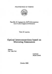
build sensors, modulators, microlasers, memories and slowlight elements [6]. We are interested in the use of microring resonators as switching devices, as proposed in [3], [4], [7]. In this context, we propose new interconnection architectures using microring resonators as optical Switching Elements (SEs). In a microring resonator SE (see Fig. 1(a)), an incoming optical signal can be either coupled to the ring (if the input signal wavelength is equal to the resonance wavelength of the microring) or it can continue along its path (if the input signal wavelength is different from the resonance wavelength). Microring resonators show intrinsic asymmetric power penalties, because optical signals traveling across the ring suffer larger power penalties than the signals that are not coupled into the ring [8]. In classical interconnection networks (both electronic and photonic), input signals usually present power losses that are independent of the state of the interconnection networks. On the contrary in microring-based interconnection networks, it is crucial to minimize the number of times an input signal is coupled into a ring while traveling through the interconnection network, since it penalizes the signal as it propagates to the corresponding output. Hence, to maximize scalability, we propose different architecture designs and a suitable control algorithm able to cope with microring physical impairments. In Sec. II, we first describe simple SEs based on microring resonators that can be used as building blocks to create interconnection networks. In Sec. III, we investigate scalability in terms of cost and performance of three classical networks based on microring SEs. To optimize the trade-off between cost and performance, we also propose two new multistage networks in Sec. IV and the mirroring technique in Sec. V. In Sec. VI we present a variation of the classical Paull’s algorithm for Clos networks [9], that configures microringbased switching fabrics and drastically reduces the probability of occurrence of highly impaired states in the switching fabric. Finally, we present some design evaluation of the proposed solutions in Sec. VII, and we draw some conclusions in Sec. VIII. II. M ICRORING - BASED SWITCHING ELEMENTS Microring resonators are basically composed by a waveguide bent to itself in a circular shape, coupled to one or two waveguides or to another microring. Fig. 1(a) shows an example of a microring coupled to two waveguides to build a 1 × 2 SE. This basic building block is called 1B-SE. Optical
signals entering the input port can be deflected to the drop port, when the ring is properly tuned (or in resonance) with the input signal wavelength, or just continue along the input waveguide towards the through port in the normal untuned state. Experimental measurements [10] show that the 1B-SE presents an asymmetric behavior. In that particular case, for microrings controlled through laser pumps, input signals sent to the drop port experience larger power losses (around 1.5 dB) than signals routed to the through port (low enough to be negligible) because of the propagation inside the ring and the ring-waveguide coupling. Regarding the crosstalk, the same study shows that the extinction ratios are different for through and drop ports; so the interfering signals present in output ports due to power leakages are different in both states; this leads to an unbalanced coherent crosstalk accumulation when several SEs are cascaded, as it happens in large-scale interconnection networks. In switching applications, microring resonators must be tuned to change their switching state. Indeed, it is possible to change the microring effective refractive index (and hence their resonance frequency) exploiting thermal-optic [11], carrier injection [12] effects, or by means of optical pumps [10]. Depending on the technology used, different tuning times, as well as different power penalties, can be observed. In the remainder of the paper, we assume that microrings are controlled by carrier injection techniques because they ensure (fast) switching times of few hundred ps [12]. We also assume a single wavelength operation; the incoming optical signal is either coupled or not to the ring depending on the wavelength to which the ring is tuned to. All the proposed architectures can be extended to a Wavelength Division Multiplexing (WDM) scenario, assuming to use the wavelength striping technique, and that the WDM channel comb fits exactly the period of the microring transfer function. A physical model of microrings, as the one presented in [4], is outside the scope of this work. Here, we simply assume that the 1B-SE can be either in a High-Loss State (HLS), or in a Low-Loss State (LLS). Indeed, we wish to study interconnection network architectures able to scale to large sizes by reducing the number of SEs in HLS that optical signals should cross while moving from input to output ports. Building up on the 1B-SE structure, it is possible to design more complex SEs that can be used as building elements in interconnection architectures. Fig. 1(b) depicts a possible implementation of a basic 2 × 2 SE (called 2B-SE). The 2B-SE exploits two 1B-SEs jointly controlled to provide two switching states. In the bar state (in1 → out1 , in2 → out2 ), each ring deflects the corresponding optical input signal to the drop port of the respective 1B-SE. In the cross state (in1 → out2 , in2 → out1 ), each ring lets the corresponding optical input signal pass to the through port of the respective 1BSE. Hence, also the 2B-SE exhibits an asymmetric behavior, because the bar state is a HLS, and the cross state is LLS with negligible power losses, as also experimentally measured in [7]. Finally, we propose a modified version of the 2B-SE, useful
in 0
out 0 in 0
Ring 1
out 0 Ring 1
Drop Port
Ring in 1
Pin
in 1
Through Port
Through Port
Ring 2
out 1
Ring 2
out1
(a) 1×2 Basic SE (1B- (b) 2 × 2 Basic SE (c) 2 × 2 Mirrored SE (2MSE) (2B-SE) SE) Fig. 1.
Elementary microring-based switching elements
to optimize the design of multistage interconnection networks. Fig. 1(c) shows a 2×2 Mirrored-SE (called 2M-SE); By crossconnecting input ports, the bar state is now realized by setting up the internal 2 × 2 SE in the cross state (LLS), whereas the cross state is achieved with an internal bar state (HLS). III. BASIC M ULTISTAGE A RCHITECTURES The SEs presented in Sec. II can be used as building elements to assemble a larger interconnection network with N input and N output ports. The network must be configured to support a given set of input-output pairs defined by a permutation π: input i must be connected to output π(i). When we say that a connection from i to π(i) must be established, we mean that a packet from input i must be transferred to output π(j) according to the decision of an external packet scheduler. The sequence of SEs traversed by the connection, defines a path in the switching network. Note that we borrow some terminology from the circuit-switching domain, but our scenario is packet switching. We aim at maximizing the scalability for large switching fabrics in terms of cost (i.e., the number of used microrings) and performance. The cost, denoted by C, is evaluated with the total number of microrings present in the network. The performance is evaluated through the maximum number of SEs configured in HLS that the input signal must cross in the optical interconnection, considering all possible input-output permutations. Such number is denoted by X and referred as the power penalty index. The best scalability is achieved by minimizing both C and X for a given N . We will consider a network design constrained by a given maximum power ˆ equal to the maximum number of HLS penalty index X, SEs that optical signals are allowed to cross. Whenever X ≤ ˆ then all the possible input-output permutations can be X, ˆ there will exist established. On the contrary, when X > X, some permutations for which some input-output connections cannot be established, since the corresponding path would ˆ in such a case, the connection is said violate the target X; to be blocked, and the corresponding packet will not be sent across the switching fabric. A. Crossbar networks based on microring resonators Firstly, we discuss the properties of the crossbar (XBAR) architecture, which will be used also as basic building block for the new architectures that will be later proposed. Crossbars can be built exploiting 1B-SEs: Fig. 2 shows an example of
k×k n×n
1
1
.. .
.. .
n×n 1
...
a
i
j
...
.. .
.. .
b
k
k
...
input stage
output stage
n middle (switching) stage
Fig. 2. 4 × 4 microring-based crossbar connecting 1 → 4, 2 → 2, 3 → 1 and 4 → 3
Fig. 3.
Rearrangeable non-blocking Clos network TABLE I
crossbar, in which column waveguides are attached to the input ports and row waveguides to the outputs. The crossbar exhibits the best performance scalability, because each input can be connected to any output crossing a single 1B-SE in HLS. Hence, the maximum number of SEs in HLS that any optical signal crosses is XXBAR (N ) = 1. However, the crossbar exhibits the worst scalability in terms of cost, since CXBAR (N ) = N 2 . As a consequence, the crossbar requires a large footprint, and a large number of SEs must be controlled, although via a simple routing algorithm. The definition of non-blocking networks less costly than the crossbar, naturally leads to multistage interconnects; we consider Clos networks and Benes networks, and we later introduce some variations to these architectures to achieve the best scalability in terms of cost and performance. B. Clos networks based on microring resonators Clos networks [9] are well-known multistage interconnection networks, whose cost scalability is better than the one of the crossbar. Fig. 3 shows a symmetric three-stage Clos network: each SE of the first stage and of the third stage is connected with all the SEs of the middle stage. The first design parameter is the number of SEs in the first and the third stage, denoted by k. The second design parameter is the number of SEs in the second stage, affecting the blocking property. In the following, we consider n = N/k SEs in the middle stage since this is the minimum n that guarantees a non-blocking rearrangeable network. As a consequence, the first and third stage SEs are of size n × n, and the second stage of SEs are of size k × k. When all SEs are implemented by crossbars, XCLOS √ = 3 and the minimum network √ cost, 3 obtained for n = N/2, is equal to CCLOS (N ) = 2 2N 2 . C. Benes networks based on microring resonators Benes networks are Clos networks that are recursively constructed with basic SEs of size 2 × 2; it must hold N = 2h for some integer h. From the cost point of view, they offer the best scalability, being asymptotically optimal [9]. In general, an N × N Benes network has a number of stages (columns
C OMPARISON BETWEEN
DIFFERENT NETWORK ARCHITECTURES , HAVING DEFINED
Network Crossbar Clos Benes M-Benes HCB M-HCB HBC M-HBC
ˆ ˆ = 2(X−1)/2 k .
Cost N2 √ 3 2 2N 2 2N log2 N − N 4N log2 N ˆ + N (X ˆ − 2) 2N 2 /k ˆ2 + 2N (2X ˆ − 3) 4N 2 /k ˆ + N (X ˆ − 1) N 2 /k ˆ2 + 2N (X ˆ − 2) 4N 2 /k
Power penalty ˆ 1≤X ˆ 3≤X
ˆ 2 log2 N − 1 ≤ X ˆ log2 N ≤ X ˆ ≤ 2 log N − 1 3≤X 2 ˆ ≤ log N 3≤X 2 ˆ ≤ 2 log N − 1 1≤X 2 ˆ ≤ log N + 1 3≤X 2
of 2B-SEs) equal to 2 log2 N − 1, each stage including N/2 basic 2B-SEs. Hence, the cost scales as CBENES (N ) = 2N log2 N − N
(1)
because each 2 × 2 SE includes 2 rings. In terms of performance, XBENES (N ) = 2 log2 N − 1 (2) since in the worst case there exists a path that passes through a HLS SE in each stage. Hence, Benes networks show a poor performance scalability, since XBENES grows with the size N ; ˆ for the power penalty index, it is given a maximum value X ˆ impossible to build networks with size N > 2(X+1)/2 . IV. H YBRID M ULTISTAGE ARCHITECTURES The upper part of Table I provides a synoptic overview of the cost and the performance for the basic architectures. To improve scalability for large N , we now combine the Clos network architecture (based on simple crossbar with good performance scalability) with the Benes network (with optimal cost scalability), considering two possible variants: i) the Hybrid Crossbar-Benes network and ii) the Hybrid BenesCrossbar network. A. The Hybrid Crossbar-Benes (HCB) architecture The HCB network is depicted in Fig. 4 and it consists of a Clos network in which the middle-stage modules are implemented through Benes networks, instead of crossbars. Like
n×n crossbar ... .. .
1
k×k Benes
.. .
...
2
.. .
2
2
2
.. .
n×n crossbars
...
.. .
.. .
.. .
...
k
.. .
... .. .
...
.. .
1
...
... .. .
1
h 1
...
1 .. .
h
1
n×n crossbar
... .. .
...
.. .
n
k
k−1
.. .
...
k Fig. 4.
Hybrid Crossbar-Benes (HCB) network. Fig. 5.
the original Clos network, the HCB network is constrained to N = nk, being n ≥ 2 the size of the crossbars, and k = 2h the size of the Benes networks for some integer h ≥ 1. Clearly, from the cost perspective, the best solution is to make the Benes network as large as possible, up to k = N/2, when the HCB network degenerates into a Benes network. On the contrary, from the performance perspective, since XHCB = 2 log2 (N/n) + 1
(3)
we must increase the crossbar size n. Thus, given a target ˆ having ˆ ≥ 3, it must satisfy XHCB ≤ X ˆ and n ≥ N/k, X ˆ (X−1)/2 ˆ ˆ defined k = 2 . The value n = N/k ensures both feasibility and minimum cost. Finally, ˆ XBAR (n) + nCBENES (k) ˆ = ˆ = 2kC CHCB (N, X) 2 2 N N ˆ − 2) = 2 + N (2 log2 kˆ − 1) = 2 + N (X ˆ k kˆ N2 ˆ − 2) (4) + N (X ˆ 2(X−3)/2 ˆ ≤ 2 log2 N − 1. Note that (4) is lower than a for 3 ≤ X ˆ ˆ − 2)/(1 − 2−(X−3)/2 crossbar for N ≥ (X ). B. The Hybrid Benes-Crossbar (HBC) architecture The HBC network is depicted in Fig. 5 (with N = n2h ) and it consists of a Benes network factorized until a certain level h ≥ 0, when the middle stage is substituted by k = 2h crossbars of size n. Again, from the cost perspective, we must increase the “Benes part” up to k = N/2 when the HBC degenerates into a Benes network. However, from the performance point of view, since XHBC = 2h + 1 = 2 log2 (N/n) + 1 (5) the best solution is to decrease the level of factorization h (up to h = 0 when the HBC degenerates into a crossbar). Thus, ˆ ≥ 1, it must be XHBC ≤ X ˆ and to satisfy a given target X ˆ having defined kˆ = 2hˆ and h ˆ = (X ˆ − 1)/2. The n ≥ N/k,
Hybrid Benes-Crossbar (HBC) network.
value n = N/kˆ ensures both feasibility and minimum cost. Now the HBC cost scales as: ˆ XBAR (n) + 2(2h)(N/2) ˆ ˆ = kC CHBC (N, X) = 2 2 N N ˆ − 1) = ˆ − 1) (6) + N (X + N (X ˆ ( X−1)/2 ˆ 2 k ˆ ≤ 2 log2 N − 1. Note that (6) is asymptotically half for 1 ≤ X the cost of the HCB and it shows a complexity lower than a ˆ ˆ − 1)/(1 − 2−(X−1)/2 crossbar for N ≥ (X ). V. M IRRORED ARCHITECTURES To further improve the scalability of multistage networks, i.e., either to reduce the power penalty index X or to achieve ˆ we larger N for a given maximum power penalty index X, propose the mirroring technique that exploits the spatial dimension, as shown in Fig. 6(a). We use two different switching planes, topologically identical: the normal plane is built with 2B-SEs only, whereas the mirrored plane with 2M-SEs only. Depending on the architecture, all inputs are connected to both planes by means of either: (i) the 1B-SE (Fig. 1(a)) which implicitly introduces a power penalty asymmetry to the signal between both planes, or (ii) the plane selector depicted in Fig. 6(b), which introduces a constant power penalty to both planes, or (iii), when possible, integrating the selector with an extension of the first stage of the architecture. However, each output merges passively the information from both planes by means of a coupler, which introduces a negligible performance impairment with respect to the plane selector. Since a HLS SE configuration in one plane corresponds to a LLS one in the other plane, all input/output connections that would cross X 2B-SEs in HLS in the normal plane can be routed on the mirrored plane along the same path, crossing (S − X) 2M-SEs in HLS, where S is the total number of traversed 2 × 2 SEs in each plane; whenever X > S/2, the routing algorithm will choose the path along the mirrored plane, with lower power penalty. As a consequence, we can start from a plane characterized by a power penalty index X
Inputs 1
N
Outputs 1
Normal plane
Normal plane out
Mirrored plane
Mirrored plane out
N
(a) Mirrored architecture Fig. 6.
ini
(b) Plane selector
Mirrored architecture and plane selector
and build the whole network with power penalty index: XM = ⌊X/2⌋ + XS
(7)
Let N be the maximum size of a Benes network satisfying ˆ let us recall (2): X ˆ = 2 log2 N − 1. A mirrored version X; ˆ satisfying X is built with two Benes networks in which the ˆ − 1, according maximum power penalty is relaxed up to 2X to (8). Hence, such Benes networks can have up to N ′ ports ˆ − 1 = 2 log2 N ′ − 1. By simple algebra, compatible with 2X it can be shown that N ′ = N 2 /2, i.e. the mirroring technique allows to scale the network by a quadratic factor. The final cost is simply obtained by considering the plane selectors and the two Benes networks: CM-BENES (N ) = 2CBENES (N ) + 2N = 4N log2 N B. Mirrored HBC networks
where XS is the power penalty introduced by the selector; as a consequence, the power penalty is roughly halved by doubling the cost of the “Benes part” of the network, constituted only by 2 × 2 SEs (i.e., doubling the number of 2 × 2 SEs). This ˆ as allows to scale the size of the network given the same X, shown below for each architecture. From the routing point of view, computing the path in the mirrored architecture has the same complexity as computing it for just a single plane, since the corresponding 2×2 SE states in normal and mirrored plane are identical. Note that mirroring the crossbars (based on 1B-SEs) does not provide any advantage in terms of power penalty. Two possible solutions to build the crossbars are possible: (i) the crossbars are replicated in both two planes; (ii) each crossbar is shared between the two planes, by adding one passive coupler at the inputs of each crossbar, and one plane selector at the outputs. Solution (i) has the advantage of avoiding additional power penalty, but it introduces the cost of replicating the crossbars. On the contrary, solution (ii) shows a larger power penalty, but this is compensated by a smaller cost. In the following, we have considered solution (i); solution (ii) is left for future works. In the following, the mirroring technique will be denoted with the prefix M- and it is applied to Benes, HCB and HBC networks. A. Mirrored Benes networks In the M-Benes network, a selector is needed and it is either a 1B-SE or the plane selector of Fig. 6(b). On the one hand, the 1B-SE introduces an asymmetric behavior in terms of power penalty, and makes more complex the layout to connect directly the drop port and the through port to each of the two planes. On the other hand, the plane selector adds a constant power penalty of one extra 1B-SE in HLS to all the signals, but may be simpler to implement due to its layout suited for an homogeneous selection between both planes. Therefore, we consider the plane selector for the M-Benes. Since the Benes network presents an odd number of stages, when we build a plane with a maximum power penalty XBENES , from (7) we obtain a M-Benes network with: XM-BENES =
XBENES − 1 + 1 = log2 N 2
(8)
The M-HBC network requires a selector due to the Benes part at the edges of the network. Similarly to the M-Benes network, we use the plane selector of Fig. 6(b). Let XHBC be the maximum power penalty in a single plane HBC network. Due to the even number of Benes stages that compose the HBC network and the single crossbar stage in the middle, we obtain the following performance for the M-HBC network: XHBC + 1 N XM-HBC = + 1 = log2 +2 (9) 2 n ˆ be the maximum power penalty satisfied in a HBC Let X network. According to (9), we can build a M-HBC in which ˆ − 3. Therethe maximum power penalty is relaxed up to 2X ˆ (X−1)/2 ˆ fore, recalling that k = 2 , the cost scales as: ˆ = 2CHBC (N, 2X ˆ − 3) + 2N = CM-HBC (N, X) 2 2 N ˆ − 2) = N + 2N (X ˆ − 2) (10) 4 + 2N (X ˆ 2X−3 kˆ2 ˆ ≤ log2 N + 1. Note that for high values of N , (10) for 3 ≤ X ˆ > 5. is convenient with respect to (6) for a power penalty X C. Mirrored HCB networks Differently from the mirrored versions of Benes and HBC networks, it is possible to integrate the plane selector in the first stage crossbar. Indeed, in a mirrored HCB network, the first stage is composed by crossbars of size n × n. The plane selector is connected to two crossbars (one for each plane) and allows to connect each input port with 2n output ports (n for each plane). This observation suggests a possible way to integrate n plane selectors and two n × n first-stage crossbars with just a a single n × (2n) crossbar, reducing the cost by 2N and the power penalty by one. Let XHCB be the maximum power penalty in a single plane HCB network. Due to the odd number of Benes stages that compose the HCB network and the crossbars stages at the edges, we obtain the following performance for the M-HCB: XM-HCB =
XHCB + 1 N = log2 +1 2 n
(11)
ˆ be the maximum power penalty satisfied in a HCB Let X network. According to (11), we can build a M-HCB in
ˆ − 1. which the maximum power penalty is relaxed up to 2X ˆ (X−1)/2 ˆ Therefore, recalling that k = 2 , the cost scales as: ˆ = 2CHCB (N, 2X ˆ − 1) = CM-HCB (N, X) 2 2 N ˆ − 3) = N + 2N (2X ˆ − 3) (12) 4 + 2N (2X ˆ 2X−3 kˆ2 ˆ ≤ log2 N + 1. Note that for high values of N , (12) for 3 ≤ X ˆ > 3. is convenient with respect to (4) for a power penalty X VI. P OWER - PENALTY- AWARE ROUTING ALGORITHM In Sec. III we have proposed different network architectures, whose cost and performance have been summarized in Table I. Independently of the configuration algorithm, both the crossbars and the Clos networks experience a fixed power penalty: XXBAR = 1 and XCLOS = 3. On the other hand, for all the other networks considered in this paper, the power penalty depends on the path chosen by the routing algorithm to establish the required connections. In this section, we show the design of a routing algorithm, aware of HLS and LLS states, that reduces the power penalty. Aim of the routing algorithm is to configure the state of each SE to satisfy any given input-output permutation π. We consider the well-known Paull algorithm [9] which has been designed to configure a three-stage Clos network, but it is also suitable for multi-stage interconnection networks based on recursive Clos construction. At each recursion level, the network is abstracted as an equivalent three stage Clos network. Referring to Fig. 3, consider a basic Clos network with Istage and III-stage modules of size n × n; as a consequence, n modules are present in the II stage. The algorithm starts from the N × N network and from a given permutation π of size N , and it computes the configuration of all the 2k + n switching modules to establish all the connections of π. Then, if the middle-stage modules are, internally, Clos networks, the Paul algorithm is applied recursively to each individual k × k module to establish all the connections of a permutation π ′ of size k computed in the external recursion level. Consider now just a basic Clos network that must be configured according to π. The Paull algorithm works in an incremental way, considering the inputs in an arbitrary order. When input x is considered, the algorithm computes the path to connect x to output π(x) by configuring (see Fig. 3): (i) the first-stage SE where input x is placed (we denote this as “module i”), (ii) the third-stage SE where output π(x) is located (we denote this as “module j”), (iii) one or two SEs present in the second stage. By construction, exactly one of the two cases can occur: 1) there exists a II-stage module a that can be connected to both modules i and j; in this case, II-stage module a is configured to support the connection from its internal input i to its internal output j; I-stage module i is configured to connect input x to its internal output a; III-stage module j is configured to connect its internal input a to π(x);
2) otherwise, there exist two II-stage modules a and b, such that a can be connected to module i, and b can be connected to module j; in this case, the algorithm moves a set of pre-existing connections from a to b and viceversa, and recomputes accordingly the configurations of the Istage modules and III-stage modules; then either a or b is used to support the new connection from x to π(x), similarly to the previous case. The Paull algorithm can exploit many degrees of freedom to establish the connections given by π: (i) the sequence of inputs considered by adding the connections in π, (ii) the choice of a and b, (iii) the choice of the paths to be moved from/to a and b. Of course, each routing choice affects the power penalty experienced by the paths across the switching fabric. We propose to modify the Paull algorithm to exploit such degrees of freedom in choosing a and b, among all the n possible II-stage modules, to minimize the power penalty. This modified version of the algorithm will be denoted by PPAPaull (Power-Penalty-Aware Paull algorithm), in contrast with the classical version denoted simply by Paull. In the case n > 2, the I-stage and III-stage modules are crossbars and the power penalty introduced by them is always two, independently from the choice of the II-stage module. Hence, PPAPaull chooses randomly a II-stage module that is currently available. In the case n = 2 (i.e. 2B-SEs at the I-stage and III-stage), the power penalty depends on the state of I-stage module i and III-stage module j. Let us assume that all the inputs and the outputs of the whole Clos network are numbered in increasing order starting from 1 and that the II-stage module a is the upper module, whereas b is the lower one. When an odd input is connected to an odd output, PPA-Paull will choose (if available) b to configure both 2B-SEs at the edges in LLS. Analogously, when an even input is connected to a even output, a will be chosen. Otherwise, either a or b will be chosen at random, since exactly one 2B-SE in the I-stage or III-stage will be in HLS (i.e., the power penalty will be always one). VII. N UMERICAL EVALUATION In Sec. VII-A we investigate the design of interconnection networks by comparing the cost and the performance. In Sec. VII-B we investigate by means of simulation the performance improvement offered by the PPA-Paull algorithm with respect to the classical Paull algorithm. A. Interconnection network design We compare N ×N interconnection networks by evaluating both the performance (in terms of power penalty index X) and the cost (in terms of number of microrings). Fig. 7 shows the power penalty of different networks in function of N . Crossbars and Clos networks show a fixed power penalty index, as expected. On the contrary, the Benes network shows the worst scalability in performance, because X scales logarithmically with respect to the number of inputs, coherently with (2). The HCB and the HBC networks (for the two different cases n = 16 and n = 32) show the same
XBAR Closs Benes M-Benes HBC/HCB n=16 HBC/HCB n=32 M-HBC/M-HCB n=32 M-HBC/M-HCB n=16
30 25
104 Cost
X
20
XBAR Clos Benes M-Benes HBC M-HBC HCB M-HCB
15
107
103
10
106 105
5
104
2
0
4
2
5
2
2
6
7
2
8
9
2
2
2
10
2
11
12
13
2
2
10
2
4
N Fig. 7.
Fig. 9.
XBAR Clos Benes M-Benes HBC M-HBC HCB M-HCB
Cost
104
Power penalty index
8
10
103
107 106 5
10
102 4 2
Fig. 8.
104
2
5
2
6
10
2
7
2 N
11
2
12
2
2
8
13
2
14
2
9
2
15
2
16
2
5
2
6
210
7
2 N
211
212
2
8
213
214
9
2
215
216
210
ˆ = 15 Cost for maximum power penalty index X
crossbars in HBC/HCB networks must be larger. On the ˆ is larger, the size contrary, Fig. 9 shows that, if the target X of crossbars inside the HBC and HCB networks decreases, reducing the overall cost. Mirrored hybrid architectures reduce by a square factor the size of the internal crossbars. For low ˆ the mirroring technique becomes cost-effective values of X, for smaller N . HCB and HBC networks are feasible whenever the Benes network violates the HLS constraint. Among the two hybrid solutions, the HCB architecture exhibits a larger complexity than HBC network, and similar observations hold for their mirrored solutions.
2
210
ˆ =7 Cost for maximum power penalty index X
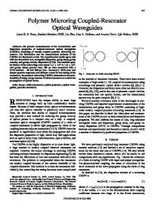
scalability law, as described by (3) and (5). As shown in Sec. V, the mirrored technique roughly reduces X by a factor of two. Thus, if we impose a maximum power penalty index ˆ it is possible to build Benes networks with a number of X, ports equal to N 2 /2 instead of N ; similar gains apply to the Benes part of the other networks. Note that this advantage appears only for large N , as predicted by our models. Fig. 8 and Fig. 9 show the cost for different interconnection networks for two different values of maximum power penalty; the points refer only to feasible configurations, that is, compatˆ The main figure refers to smaller ible with the given target X. networks (N ranging from 24 to 210 ), whereas the inset figure refers to larger networks (N from 210 to 216 ). In general, the crossbar always shows the highest cost, while Benes networks always the lower one, whenever feasible. Fig. 8 shows that the only feasible Benes network, when ˆ = 7, is for N = 16. Instead, exploiting the mirroring X technique, networks up to N = 128 can be built. Clos networks show the lowest complexity for very large N . Indeed, as the network size increases, the worst case power penalty ˆ is smaller, edge or inner grows. As a consequence, when X
B. The performance of the routing algorithm We compare the performance of the PPA-Paull algorithm with respect to the classical version of the Paull algorithm. We report results only for Benes networks, which provide an upper bound on the power penalty experienced by the other architectures. We assume a microring based interconnection network, in synchronous operation, i.e., time is divided into intervals of fixed duration (timeslots) and the network transfers data units of fixed size (cells); the timeslot duration is equal to the transmission time of a cell. In the case of variable-size packets, incoming packets are chopped into cells, while outputs reassemble all the cells belonging to the same packet. We consider a uniform traffic scenario, with ρ being the average load at each input port. At each timeslot, we generate an input-output permutation π in which each input is active with probability ρ. Starting from a random input and considering all the other inputs in a sequential fashion, a sequence of consecutive connections is generated according to the rule: if input i is active, it is connected to π(i). The routing algorithm adds each connection at the time in an incremental way, during the same timeslot. Each path computed by the algorithm will result in a certain ˆ the power penalty index; if such index is larger than X, corresponding connection is blocked. To compare the routing ˆ as the algorithms, we measure the blocking probability PB (X)
0
10
0
0.9 0.5
10
10-1 0.1
10
1 0.99
10-2 -2
10
ˆ) PB(X
Throughput
-1
Paull (ρ=0.9) Paull (ρ=0.5) Paull (ρ=0.1) PPA-Paull (ρ=0.9) PPA-Paull (ρ=0.5) PPA-Paull (ρ=0.1)
10-3 10-4 0
2
4
6
0.98
-3
0.97
10
0
0.5
1
1.5
2
PPA-Paull (N=32) PPA-Paull (N=64) PPA-Paull (N=128) -5 Paull (N=32) 10 Paull (N=64) Paull (N=128) 0 0 2 4 -4
10
8
10
6 ˆ X
ˆ X Throughput under uniform traffic for N = 64.
average fraction of blocked input-output pairs over the number of active inputs. As a complementary measurement, the throughput is evaluated as the average number of connections that are established without blocking in a generic timeslot; the maximum throughput is equal to the average load ρ and it is reached when a connection is never blocked, for any permutation. In the figures, the throughput and the blocking probability are averaged across many timeslots. Fig. 10 shows the throughput in function of the maximum ˆ for a 64 × 64 Benes network and different power penalty X input loads: ρ ∈ {0.1, 0.5, 0.9}, corresponding to a lightly, medium and highly loaded network, respectively. For enough ˆ the throughput reaches its maximum value (0.1, 0.5 or large X, 0.9 for each couple of curves), since the routing is not affected by the power penalty; in such case, all the algorithms behave the same. Note that the number of stages for the considered ˆ are not network is S(64) = 11, hence larger values of X ˆ affecting the routing. On the other side, smaller values of X reduce the possibility of finding feasible paths; in the extreme case, the throughput approaches zero. In general, PPA-Paull achieves always a better throughput than Paull. When the input ˆ to achieve the maximum load ρ increases, the minimum X throughput increases, since the routing is more constrained by a larger number of preliminary paths added during the current timeslot. Fig. 11, Fig. 12 and Fig. 13 show the blocking probability in function of the maximum power penalty, each figure referring to a different value of input load. The smaller plot inside each ˆ figure details the blocking probability for low values of X. The total number of stages S(N ) in function of N are S(32) = 9, S(64) = 11 and S(128) = 13; whenever ˆ > S(N ), the blocking probability is zero by construction X and the maximum throughput is achieved. On the contrary, ˆ approaches zero, the routing is severely constrained when X by the power penalty: the blocking probability increases and the throughput tends to zero. Furthermore, as N increases, in all the figures the blocking probability increases due to the larger network depth. In general, the reduction in the blocking
10
12
Fig. 11. Blocking probability in Benes networks under uniform traffic with ρ = 0.1 0
10
10-1 1
-2
10 ˆ) PB(X
Fig. 10.
8
0.99 0.98
10-3
0.97
0
0.5
1
1.5
2
PPA-Paull (N=32) PPA-Paull (N=64) PPA-Paull (N=128) Paull (N=32) Paull (N=64) Paull (N=128)
-4
10
10-5 0 0
2
4
6
8
10
12
ˆ X Fig. 12. Blocking probability in Benes networks under uniform traffic with ρ = 0.5
probability due to PPA-Paull with respect to Paull is very large, reaching more than two orders of magnitude in some cases. To better understand such results, consider the case in which just one path must be connected (this event may happen for ˆ = 0, there will be only one low input load). If we set X specific destination (among N possible ones) reachable by each input; the corresponding path will be found by PPAPaull. Thus, at low load and under uniform traffic, we can expect PBPPA-Paull (0) = 1 − 1/N (consistently with the values in the figure). Now observe that, in a Benes network, there exist always 2log2 N −1 = N/2 different paths connecting any input to any output, since in the first log2 N − 1 stages there are always two output ports in each module that can be used to reach any destination, whereas in the last log2 N stages there exists just one output port in each module to reach the desired output. Given an input-output pair with a possible path compatible ˆ = 0 (this pair is chosen with probability 1/N as with X shown above), the Paull algorithm will choose one random path among the N/2 available paths, but only one of them
0
ACKNOWLEDGMENTS
10
This work was partially supported by the BONE project, a Network of Excellence funded by the European Commission within the 7th Framework Programme.
-1
10
1
-2
0.99
ˆ) PB(X
10
R EFERENCES
0.98
-3
10
0.97 0
0.5
1
1.5
2
PPA-Paull (N=32) PPA-Paull (N=64) PPA-Paull (N=128) Paull (N=32) Paull (N=64) Paull (N=128)
-4
10
10-5 0 0
2
4
6
8
10
12
ˆ X Fig. 13. Blocking probability in Benes networks under uniform traffic with ρ = 0.9
ˆ = 0. Hence, we can will be able to satisfy the constraint X Paull 2 expect that PB (0) = 1 − 2/N (coherently with the values in the figure), which is larger than PBPPA-Paull (0). We now evaluate the maximum power penalty experienced by a single path computed by PPA-Paull. At each factorization level, PPA-Paull chooses the configuration of the first and the third stage to minimize the power penalty; in the case of a single path, the power penalty can increase by one at each factorization level. As a consequence, the maximum power penalty will be log2 N − 1, equal to the number of factorization levels. Hence, for low load, we expect that the ˆ ≥ log2 N . Indeed, blocking probability tends to zero when X Fig. 11 shows that the observed blocking probability goes to ˆ = 6, 7, 8 when N = 32, 64, 128, which is very zero for X close to the bound found before.
VIII. C ONCLUSIONS In this paper we analyzed the scalability in terms of cost and performance of different interconnection networks based on microring resonators. We described the basic 1 × 2 and 2 × 2 switching elements, and we highlighted the asymmetric power penalty of the different switching states. Then, we analyzed the effects of these asymmetries on the cost and feasibility of crossbar, Benes and Clos networks. To achieve a better compromise between costs (in terms of switching elements) and performance (in terms of power penalty), we proposed (i) two architectures based on different combinations of the Benes and crossbar networks and (ii) the mirroring technique. Finally, we proposed a simple variation of the classical Paull algorithm to set up new connections, and we investigated the corresponding improvement in terms of the power penalty. Given the promising results obtained in our studies, we believe that the role of microring resonators in future high capacity photonic interconnection networks will become more and more relevant.
[1] M. Haurylau, G. Chen, H. Chen, J. Zhang, N. A. Nelson, D. H. Albonesi, E. G. Friedman, and P. M. Fauchet, “On-chip optical interconnect roadmap: Challenges and critical directions,” IEEE Journal of Selected Topics in Quantum Electronics, vol. 12, no. 6, pp. 1699–1705, November 2006. [2] A. V. Krishnamoorthy, X. Z. R. Ho, H. Schwetman, J. Lexau, P. Koka, G. Li, I. Shubin, and J. E. Cunningham, “The integration of silicon photonics and vlsi electronics for computing systems intra-connect,” in Photonic in Switching, 2009. [3] M. Petracca, B. G. Lee, K. Bergman, and L. P. Carloni, “Design exploration of optical interconnection networks for chip multiprocessors,” in Hot Interconnects, 2008, pp. 31–40. [4] A. Bianco, D. Cuda, R. Gaudino, F. Neri, G. Gavilanes, and M. Petracca, “Scalability of optical interconnects based on microring resonators,” IEEE Photonic Technology Letters, vol. 22, no. 15, pp. 1081–1083, July 2010. [5] S. I. Association, “International technology roadmap for semiconductors,” http://www.itrs.net/Links/2009ITRS/Home2009.htm. [6] L. Tobing and P. Dumon, Photonic Microresonator Research and Applications. Springer, 2010, pp. 1–23. [7] B. G. Lee, A. Biberman, N. Sherwood-Droz, C. B. Poitras, M. Lipson, and K. Bergman, “High-speed 2x2 switch for multi-wavelength message routing in on-chip silicon photonic networks,” in European Conference on Optical Communication (ECOC), May 2008. [8] A. Bianco, D. Cuda, M. G. R. Gaudino, G. Gavilanes, P. Giaccone, and F. Neri, “Optical interconnects based on microring resonators,” in ICC, May 2010. [9] J. Y. Hui, Switching and traffic theory for integrated broadband networks. Kluwer, 1990. [10] B. G. Lee, A. Biberman, P. Dong, M. Lipson, and K. Bergman, “Alloptical comb switch for multiwavelength message routing in silicon photonic networks,” IEEE Photonic Technology Letters, vol. 20, no. 10, pp. 767–769, May 2008. [11] B. G. Lee, A. Biberman, N.Sherwood-Droz, M. Lipson, and K. Bergman, “Thermally active 4x4 non-blocking switch for networks-on-chip,” Annual Meeting of the Lasers and Electro-Optics Society (LEOS), p. TuBB3, Nov 2008. [12] C. Li and A. Poon, “Silicon electro-optic switching based on coupledmicroring resonators,” in Conference on Lasers and Electro-Optics (CLEO), May 2007.