Mar 3, 2015 - This makes it possible to combine more beam position monitor .... (IPs) may only be a few degrees. If in this case ... measurements at the IPs in.
PHYSICAL REVIEW SPECIAL TOPICS - ACCELERATORS AND BEAMS 18, 031002 (2015)
Optics measurement algorithms and error analysis for the proton energy frontier A. Langner CERN, CH 1211 Geneva 23, Switzerland and Universität Hamburg, Luruper Chaussee 149, 22761 Hamburg, Germany
R. Tomás CERN, CH 1211 Geneva 23, Switzerland (Received 9 September 2014; published 3 March 2015) Optics measurement algorithms have been improved in preparation for the commissioning of the LHC at higher energy, i.e., with an increased damage potential. Due to machine protection considerations the higher energy sets tighter limits in the maximum excitation amplitude and the total beam charge, reducing the signal to noise ratio of optics measurements. Furthermore the precision in 2012 (4 TeV) was insufficient to understand beam size measurements and determine interaction point (IP) β-functions (β� ). A new, more sophisticated algorithm has been developed which takes into account both the statistical and systematic errors involved in this measurement. This makes it possible to combine more beam position monitor measurements for deriving the optical parameters and demonstrates to significantly improve the accuracy and precision. Measurements from the 2012 run have been reanalyzed which, due to the improved algorithms, result in a significantly higher precision of the derived optical parameters and decreased the average error bars by a factor of three to four. This allowed the calculation of β� values and demonstrated to be fundamental in the understanding of emittance evolution during the energy ramp. DOI: 10.1103/PhysRevSTAB.18.031002
PACS numbers: 41.85.-p, 29.20.db, 29.27.Eg
I. INTRODUCTION Optics measurements and corrections are of great importance for the LHC, due to its tight design tolerances on the beam orbit and optical functions. A large effort has been put in the LHC optics commissioning and in 2012 a record low β-beating was achieved [1–6]. During the ongoing long shutdown (LS1) in 2014, improvements of the optics measurement methods are being studied. A better accuracy and precision will be needed since due to machine protection considerations the excitation amplitude and bunch intensity will be limited in 2015 which will reduce the signal to noise ratio for optics measurements. A direct way to improve accuracy and precision might be just considering more beam position monitor (BPM) data. However it is not possible to simply add more BPMs in the calculations as systematic errors would deteriorate the measurement accuracy. Using more BPMs requires an ansatz for the single phase uncertainty and a thorough analysis of systematic errors and correlations via MonteCarlo simulations. A new algorithm which allows us to reliably increase the number of BPMs in an optics measurements is described in Sec. II with a focus on its
Published by the American Physical Society under the terms of the Creative Commons Attribution 3.0 License. Further distribution of this work must maintain attribution to the author(s) and the published article’s title, journal citation, and DOI.
1098-4402=15=18(3)=031002(10)
application for the LHC. Another improvement which is used here is the cleaning of measurement data using a singular value decomposition (SVD) technique, which is applied to the BPM turn-by-turn data. Improvements of the optics model for the analysis also lead to a better precision of measured optics parameters, which is described in Sec. III. Furthermore, a more accurate calibration of wide-aperture quadrupole magnets (MQY) is used, which has been verified in a dedicated machine development session [7]. These improvements allowed to calculate β� and dispersion values for the β� ¼ 0.6m optics. With this enhanced precision it was possible to derive reliably the βvalues at the position of the wire scanners during the energy ramp. The emittance study during the energy ramp profited highly from the more accurate β-values [8,9]. The propagation of measured optics parameters to other elements is described in Sec. IV, together with an error propagation using analytic equations. In Sec. V results from reanalyzing experimental data from 2012 are presented. II. N-BPM METHOD BPMs are used to measure the turn-by-turn data of betatron oscillations, which are excited adiabatically by an AC dipole [10,11]. The phase of this oscillation can be derived by a harmonic analysis of the turn-by-turn data at every BPM position. With the phase advance and transfer matrix in between three BPMs the β-function can be calculated at the position of the three BPMs [12,13].
031002-1
Published by the American Physical Society
A. LANGNER AND R. TOMÁS
Phys. Rev. ST Accel. Beams 18, 031002 (2015) β-function, depending on the phase advances between the three BPMs. From Eq. (1) one can derive two conditions for the optimal phase advances. The phase advance from the probed BPM (i) to the other two ðj; kÞ should be
FIG. 1. Illustration of the β-function measurement from phase. The phase advances ϕi;j in between three positions si are needed to derive the β-functions at those positions.
The Twiss parameters βi and αi at the positions si can be obtained with Eqs. (1), (2) where ϕi;j ¼ ϕj − ϕi is the phase advance and Mmnði;jÞ are the transfer matrix elements from si to sj , cf. Fig. 1. ϵijk is the Levi-Civita symbol which allows for a compact notation of the three cases of deriving the Twiss parameters at the different BPMs. No summation over equal indices is implied. βi ¼
ϵijk cotðϕi;j Þ þ ϵikj cotðϕi;k Þ M
M
αi ¼
ð1Þ
M
þ ϵikj M11ði;kÞ ϵijk M11ði;jÞ 12ði;jÞ 12ði;kÞ M
ϵijk M11ði;kÞ cotðϕi;j Þ þ ϵikj M11ði;jÞ cotðϕi;k Þ 12ði;kÞ 12ði;jÞ M
M
ϵijk M11ði;jÞ þ ϵikj M11ði;kÞ 12ði;jÞ 12ði;kÞ
:
ð2Þ
The accuracy of this method depends not only on the knowledge of the optics model and the precision of the measured phase but also on the value of the phase advances between the BPMs. From Eq. (1) it can be seen that, for example, a phase advance between two BPMs should not be close to a multiple of π as the cotangent becomes infinite at those points. Figure 2 shows the propagated error of the
ϕi;j ¼ π4 þ n1 π2 ;
ϕi;k ¼ π4 þ ð2n2 þ 1 − n1 Þ π2 ;
n1 ; n2 ∈ Z:
ð3Þ
The method that has been used so far takes three neighboring BPMs for the calculation of the β-functions at these three BPM positions. In the arcs, where in general the phase advance between consecutive BPMs is about π=4, this method is already close to the optimum phase advances, when probing the middle BPM. However in the case that the probed BPM is not in the middle of the other two BPMs, the optimum would be to skip the farther BPM and use instead the next following BPM, cf. Fig. 3. In the interaction regions (IRs), the phase advances can be very different as the optics do not follow the regular focussing-drift-defocussing-drift structure of the arcs in order to fulfill other constraints, e.g., collision point focusing. For example in the ATLAS and CMS IRs, where the β-function reaches very high values, the phase advances between consecutive BPMs close to the interaction points (IPs) may only be a few degrees. If in this case only neighboring BPMs are used, this results in large uncertainties. This prevented β� measurements at the IPs in 2012 [3]. An improved algorithm is developed here, which allows us to use more BPM combinations from a larger range of BPMs. This makes it possible to include BPM combinations with better phase advances and also increases the amount of information that is used in the measurement of the β-function. A range of N BPMs is chosen centered at the probed BPM. To find the best estimate of the measured β-function from m combinations of three BPMs out of the N BPMs, a least squares minimization is performed of the function SðβÞ ¼
m X m X ðβi − βÞV −1 ij ðβj − βÞ;
ð4Þ
i¼1 j¼1
where βi are the β-functions inferred from different BPM combinations at the given probed BPM and V ij are the elements of the covariance matrix for the different βi . FIG. 2. Expected error of a measured β-function at position s1 , depending on the phase advances to the other two BPMs. The six used phase advances (three BPM combinations each for horizontal and vertical plane) for a BPM position in IR4 from the neighboring BPM method are indicated by triangles. When an increased range of 7 BPM is used (N-BPM method), 15 different combinations of phase advances are possible per plane, including the ones that are indicated by triangles. Another six better suited combinations of phase advances from the range of 7-BPMs are indicated by circles.
FIG. 3. In the arcs the phase advance between two consecutive BPMs is about π=4. If the blue BPM is probed, it is better to skip the grey BPM and use the two red BPMs. The resulting phase advances are approximately ϕ1;2 ¼ π=4 and ϕ1;3 ¼ 3π=4, which is the optimum according to Eq. (3).
031002-2
OPTICS MEASUREMENT ALGORITHMS AND ERROR … Therefore the minimization of SðβÞ is considering the individual uncertainties and correlations of the βi from the m different BPM combinations which allows for a better estimate of the β-function. The measured β-function at the probed BPM position is then a weighted average of the m β-functions β¼
m X i¼1
wi βi :
ð5Þ
From the minimization of Eq. (4) we can derive the weights Pm V −1 Pm ik −1 : wi ¼ Pm k¼1 j¼1 V jk k¼1
ð6Þ
This equation replaces the simple average introduced in [1]. The uncertainty for this measurement is σ 2β ¼
m X m X k¼1 j¼1
wj wk V jk :
ð7Þ
The higher sensitivity due to this BPM selection is illustrated for a special situation in IR4 in Fig. 2, where the used phase advances in the neighboring BPM method (∇) and in the N-BPM method (∘) are shown. The covariance matrix V is an element-wise sum of the covariance matrices for the systematic and statistical errors V ij ¼ V ij;stat þ V ij;syst :
which compensates the underestimation of the uncertainty for a small sample size. During the LHC Run I the error was calculated from a normal standard deviation without the t correction and by dividing the sum by n instead of (n-1). This has been changed since the mean value of the phase advance is also obtained from the measurements, and there are only (n-1) degrees of freedom left for the calculation of the standard deviation. Table I shows tðnÞ for different number of measurements, which shows that this correction is needed since due to limits in the beam time, the amount of measurements is always limited. The correlation between two phase advances which have one BPM in common, ϕi;j and ϕi;k , depends on the uncertainty of the single phase ϕi at the common BPM. The error of the single phase ϕi is not known, because it cannot be compared among the measurement results since its value is arbitrary and may vary. We are using the ansatz 1 σ ϕ ∼ β−2 as shown in [12] to derive the single phase uncertainties ϕi from the uncertainty of the phase advance ϕi;j based on the β-functions at the two locations si and sj σ 2ϕi
¼
σ ϕi;j
sffiffiffiffiffiffiffiffiffiffiffiffiffiffiffiffiffiffiffiffiffiffiffiffiffiffiffiffiffiffiffiffiffiffiffiffiffiffiffiffiffiffiffiffiffiffiffiffi n 1 X ¼ tðnÞ ½ϕ − ϕi;j;ðkÞ �2 ; n − 1 k¼1 i;j
ð9Þ
where ϕi;j is the average phase advance from BPM (i) to (j) and tðnÞ is the correction from the Student’s t distribution,
� � βi −1 1þ : βj
0 σ2
0
B M¼@ 0
σ 2ϕj
0
0
ϕi
ð10Þ
0 1 0 C A;
ð11Þ
σ 2ϕk
to a covariance matrix of the phase advances by using the transformation matrix 0 ∂ϕi;j
A. Statistical uncertainty of the measured β-function If Eq. (1) is used to derive the β-function, two phase advances between BPMs are used (ϕi;j , ϕi;k ) in which the BPM (i) appears twice. This introduces a correlation which must be regarded in the error propagation, since the same phase measurement at BPM (i) was used in the calculation of both phase advances. More correlations will occur when the BPM combinations to calculate the different βi in Eq. (5) have common BPMs, which all contributes to the covariance matrix V stat . The error of the measured phase advance can be derived from the standard deviation of n measurements
σ 2ϕi;j
The correlation coefficient between two phase advances ϕi;j and ϕi;k with j ≠ k can be derived by transforming the covariance matrix of the single phase uncertainties
ð8Þ
For this method it is fundamental to have a precise knowledge of these covariance matrices which will be derived in the following sections.
Phys. Rev. ST Accel. Beams 18, 031002 (2015)
∂ϕi
B B ∂ϕ T 1 ¼ B ∂ϕi;jj @ ∂ϕi;j ∂ϕk
∂ϕi;k ∂ϕi ∂ϕi;k ∂ϕj ∂ϕi;k ∂ϕk
1 C C C: A
ð12Þ
With the transformation T T1 MT 1 one gets the covariance matrix for the two phase advances ϕi;j and ϕi;k in the standard form TABLE I. 68.3%.
Values for the t correction for a confidence interval of
Number of measurements
tðnÞ
2 3 4 5 10
1.84 1.32 1.20 1.15 1.06
031002-3
A. LANGNER AND R. TOMÁS T T1 MT 1 ¼
Phys. Rev. ST Accel. Beams 18, 031002 (2015)
σ 2ϕi;j
ρðϕi;j ; ϕi;k Þσ ϕi;j σ ϕi;k
ρðϕi;j ; ϕi;k Þσ ϕi;j σ ϕi;k
σ 2ϕi;k
! ;
ð13Þ from which the correlation coefficient can be extracted as ρðϕi;j ; ϕi;k Þ ¼
∂ϕi;j ∂ϕi;k σ 2ϕi : ∂ϕi ∂ϕi σ ϕi;j σ ϕi;k
ð14Þ
Let the phase at the probed BPM be ϕ1 , all other phase advances can be calculated with respect to this BPM. The elements of the covariance matrix for the different phase advances ϕ1;2 to ϕ1;n are defined by Ci−1;j−1 ¼ ρðϕ1;i ; ϕ1;j Þσ ϕ1;i σ ϕ1;j ; i ≥ 2; j ≥ 2;
ð15Þ
which is σ 2ϕ1;i when i ¼ j and �σ 2ϕ1 elsewhere. Using the transformation matrix 0
∂β1 ∂ϕ1;2
B B T 2 ¼ B ... @
∂β1 ∂ϕ1;n
��� ..
∂βm ∂ϕ1;2
.
���
1
C .. C ; . C A
ð16Þ
∂βm ∂ϕ1;n
the covariance matrix for the phases can be transformed to a covariance matrix for the m β-functions (V stat ) which are calculated from using different BPM combinations, V stat ¼ T T2 CT 2 :
FIG. 4. Relative uncertainty of the β-function derived in the error propagation compared to a fit of the variation of calculated β-functions.
ð17Þ
This covariance matrix is to be used in Eq. (8). As a test of the correct implementation of the equations for the statistical errors in the optics analysis code, simulations of the optics measurement have been performed. Turn-by-turn BPM measurements were simulated for every BPM positions with enhanced noise and without SVD cleaning. This has been done to create 500 sets of BPM turn-by-turn data, which corresponds to 500 measurements. Since in contrast to a real measurement, in this simulation the phase at each BPM is known in absolute values, it is possible to derive the uncertainty of the phase for each BPM position from its variation. As the uncertainties of the single phases and also of the phase advances are known, they were used directly in Eq. (14) to create the covariance matrix. The aforedescribed error propagation was applied and the β-function derived according to Eq. (5), with its uncertainty according to Eq. (7). Systematic errors are neglected here as they are not depending on the amount of measurements. The distribution of the β-function in these 500 data sets has been fitted to a Gaussian for each BPM. The value of
the σ from the fit was then compared to calculated uncertainties of the β-function using Eq. (7), cf. Fig. 4. The calculated values of the uncertainty agree well to the expected value from the variations of the β-function, which is not the case for the old equations for the error calculation, where the error bars were too pessimistic. In this plot one can furthermore see that most of the points are located at two levels. This is due to the fact that the BPMs in the arcs, where most BPMs are, alternate between two β values, and the larger β-function can be measured with a higher relative precision. The simulated sets of BPM turn-by-turn data can be used to study the uncertainty of the error bar. For that purpose, several measurement files can be analyzed together, so that the phase uncertainty will be calculated from a limited amount of measurement files. This has been done in [14] for analyzing up to ten measurements together, and it was concluded that using at least five measurements is recommended. B. Systematic uncertainties The influence of deviations in the optics model to the measurement of the β-function can be determined by introducing errors in the optics model following a Monte-Carlo approach. The β-function is then calculated using the phase advances from the perturbed model and the transfer matrix elements from the ideal model. The variation of the β-functions corresponds to the error for every given set of BPM combinations. The following uncertainties are considered in the estimate of the systematic error: (i) the uncertainty of the quadrupolar error (b2 ) of the dipoles, (ii) an individual uncertainty of the gradient for each quadrupole magnet family, (iii) a Gaussian distributed misalignment uncertainty of 1 mm along the longitudinal axis for quadrupole magnets, and (iv) a Gaussian distributed misalignment uncertainty of 1 mm in the transverse
031002-4
OPTICS MEASUREMENT ALGORITHMS AND ERROR … TABLE II. Gradient errors of different quadrupole magnets in the systematic error calculation. Error relative to their main field (10−4 ) Quadrupole MQ MQM MQY MQX MQW MQT
450 GeV
4 TeV
18 13 11 4 34 73
17 12 7 4 13 77
Phys. Rev. ST Accel. Beams 18, 031002 (2015)
symmetry and regular distribution of BPMs in the arcs. It shows that the systematic error is around 0.3% when neighboring BPMs are used. It increases to up to 1.5% in most cases if one allows to skip one BPM, i.e., for a range of 7 BPM. A range of 9 BPMs is not shown in this table as the systematic error would be very large since the phase advance to the fourth BPM left or right of the probed BPM is around π. Although the systematic errors increase for larger ranges of BPMs, for a range of 11 BPMs some combinations of three BPMs can be found with uncertainties below 2%. C. Range of BPMs
plane for sextupole magnets. The gradient uncertainties for the different quadrupole families have been derived from magnetic measurements [15,16]. The distribution of the measured b2 component and its uncertainty have been fitted with a Gaussian distribution for each magnet family, see Table II. This has been done for 1000 cases where the errors have been varied following Gaussian distributions, truncated at three standard deviations. From this Monte-Carlo simulation one can derive the covariance matrix of the systematic errors V syst . In Table III the average systematic error at arc BPMs is shown for different BPM combinations. In this table several combinations of three BPMs have been omitted since they show the same results due to the
TABLE III. Systematic error of the measured β-function at arc BPMs for using different BPM combinations. The phase advance between consecutive BPMs is approximately π=4.
0.3 0.4 1.0 7.1 1.1 1.4 1.7 1.8 7.9 22.3 1.3 1.9 6.1 1.0 3.0 4.5 5.2 1.6
The described algorithm to derive the β-function at one BPM allows us in general to use the measured turn-by-turn data of all available BPMs. However the farther away two BPMs are the larger become systematic uncertainties of the transfer matrix elements and the improvement of the error bar will therefore become smaller. On the other hand the computation of the covariance matrix is more time consuming for larger ranges of BPMs. The gain in precision and accuracy was studied with simulations for a range of up to 13 BPMs and different amount of used BPM combinations. The BPM combinations were sorted according to the expected error for the β-function based on their model phase advances. This allows to exclude BPM combinations that have unsuited phase advances, for example if the cotangent in Eq. (1) becomes infinite. The BPM combinations which are used for the computation of the β-function are drawn from this sorted list starting with the combinations with the best phase advances. Another simulation was performed with a sample size of 1000, where we applied random model uncertainties according to the previous section, as well as a Gaussian noise of 200 μm to the BPM data for an oscillation amplitude of 1 mm in the arcs. From the fit of a Gaussian distribution to the variation of the β-functions at each BPM we can derive the following two parameters which describe the uncertainty of the measurement. The mean value of the distribution of the β-functions is the accuracy, as it shows a bias toward larger or smaller results. The width of the distribution is the precision which describes how much the results are spreading. The average accuracy for all BPMs is always below 0.25% which shows that the bias toward a wrong result is negligible, cf. Fig. 5. The improvement for the average precision is shown in Fig. 6. The gain in precision is very little when increasing the BPM range from 11 to 13. The amount of BPM combinations increase the precision noticeably up to using 6 BPMs and seem to saturate after that. For the calculations for the LHC in the following sections we are using 10 BPM combinations from a range of 11 BPMs, which seems to be a good compromise between computation time efficiency and precision.
031002-5
A. LANGNER AND R. TOMÁS
Phys. Rev. ST Accel. Beams 18, 031002 (2015)
FIG. 5. Accuracy of the derived β-functions from simulations for different ranges of BPMs and different amount of BPM combinations. The oscillation amplitude was 1 mm in the arcs and a Gaussian noise of 200 μm was applied.
FIG. 7. Average error bar of the experimentally measured β-function for different optics configuration at 4 TeV, except for injection at 0.45 TeV. Error bars which are larger than 50% were disregarded in the calculation of the average.
the 2012 LHC run with different optics configurations have been reanalyzed using the N-BPM method as well as an improved optics model which includes the dipole b2 errors. The new systematic error from Sec. II B was compared to the standard deviation of the three β-functions from using different BPM combinations, which has been used in the past as an estimator of the systematic errors. In Fig. 7 the average relative error bars of these measurements are shown for injection optics at 0.45 TeV and 4 TeV (flat top), a squeeze to β� ¼ 0.6 m and a squeeze to β� ¼ 0.2 m in the achromatic telescopic squeezing (ATS) scheme [18]. The β� values in this paper refer to the β-function at the ATLAS and CMS IPs. The error bars for the measured β-function are significantly reduced with the N-BPM method. FIG. 6. Precision of the derived β-functions from simulations for different ranges of BPMs and different amount of BPM combinations. The oscillation amplitude was 1 mm in the arcs and a Gaussian noise of 200 μm was applied.
III. MODEL PRECISION The calculation of β-functions from the phase advances requires knowledge of the optics model, cf. Eq. (1). Furthermore the N-BPM technique, which was described in the previous section, will also use BPMs which are farther away from the probed BPM. Therefore model uncertainties play a more important role. In this section the benefit of considering measured b2 of the LHC dipoles [17] in the model for the optics measurement is studied. For example, for injection optics at 4 TeV, including the dipole b2 errors and the corresponding corrections with the arc trim quadrupoles (MQT), shows a β-beating of around 10%. The dipole b2 errors are available for different energies from the WISE simulation [15,16]. The phase shift of the betatron oscillation due to the b2 errors is canceled arc-by-arc using the arc MQT magnets for a correction, as illustrated in [2]. Several measurements from
FIG. 8. Average error bar of experimentally measured β-functions separately for the two error contributions. Top: Error propagated from the uncertainty of the phase advance, cf. Eq. (7). Bottom: Systematic errors as described in Sec. II B. For the neighboring BPM method instead the standard deviation of the three calculated β from different BPM combinations is used. Beam energy was at 4 TeV, except for injection at 0.45 TeV.
031002-6
OPTICS MEASUREMENT ALGORITHMS AND ERROR …
Phys. Rev. ST Accel. Beams 18, 031002 (2015)
In Fig. 8 the two contributions to the final error bar of the β-function are shown separately. Using the N-BPM method reduces the error which is propagated from the uncertainty of the phase advance. For the systematic error a large decrease is observed when using the N-BPM method. This indicates that in the past, the systematic errors were in general largely overestimated. IV. PROPAGATION TO ELEMENTS In the previous sections, the measurement of optical functions was described at the BPMs. It is very important to know the optical functions also at other positions as for example at the collision points or locations of diagnostic instruments like beam wire scanners. The segment-bysegment technique is used for the propagation of optical functions [1,2]. It basically runs MADX in a part of the accelerator in between two BPM positions. The measured optical functions at the BPMs are used as start parameters for this simulation. In addition, this code is also used for finding optics corrections. For that purpose the measured phase is compared with the model phases in each segment. For the propagation of the measurement uncertainty, analytical equations are derived here. The beta-beating propagation can be described by an oscillation with constant amplitude A which propagates with twice the betatron oscillation frequency. Δβ ðsÞ ¼ A · sin½2 · ϕðsÞ þ ϕ0 � β
FIG. 10. β-beating for Beam 1 after local and global corrections at β� ¼ 0.6 m.
This error is shown in Fig. 9 versus the phase advance from the beginning of the segment. Periodic minima in the uncertainty of ϕs are observed at multiples of π. For optics correction, where the simulated phase is used, this suggests to use various segments to achieve a low uncertainty of the phase for more BPM positions. From Eq. (18) one can also derive the uncertainty of the propagated β-function
ð18Þ
Using Eq. (18) one can approximate the deviation of the phase Δϕ due to the β-beating at the start of the segment. Error propagation on Δϕ using the uncertainties σ β0 and σ α0 of the optical functions at the start of the segment leads to the uncertainty of the propagated phase � � 1 α 1 1 2 2 σ 2ϕs ¼ ½cosð2ϕÞ − 1� 0 þ sinð2ϕÞ σ β0 2 β0 β0 2 �2 � 1 ½cosð2ϕÞ − 1� σ 2α0 þ ð19Þ 2
FIG. 9. Error from Eq. (19) of the phase advance in Segmentby-Segment. For IR1 starting at BPM10.L1.B2, the position of following BPMs is indicated.
� � α 1 2 2 σ 2βs ¼ βs sinð2ϕÞ 0 þ βs cosð2ϕÞ σ β 0 β0 β0 þ ½βs sinð2ϕÞ�2 σ 2α0 :
ð20Þ
This error is now considered for the calculation of β-functions at other elements, e.g., for the β� , see Sec. V. Since this method requires knowledge of the optics model one can derive a systematic error of the propagated optical functions similar to the systematic
FIG. 11. β-beating for Beam 2 after local and global corrections at β� ¼ 0.6 m.
031002-7
A. LANGNER AND R. TOMÁS
Phys. Rev. ST Accel. Beams 18, 031002 (2015)
TABLE IV. RMS and peak β-beating after local and global corrections at β� ¼ 0.6 m. Beam 1 Δβ β ð%Þ
Beam 2
x
y
x
y
peak
9�1
9�1
7.0 � 0.6
6.7 � 1.7
rms
2.6
2.3
2.4
2.2
TABLE V. Measured β� values for squeezed optics at β� ¼ 0.6 m after local and global corrections. Beam 1 IP1 IP2 IP5 IP8 Beam 2 IP1 IP2 IP5 IP8
β� x (m)
β� y (m)
0.589 � 0.019 2.85 � 0.19 0.595 � 0.010 3.03 � 0.08
0.61 � 0.03 2.86 � 0.06 0.595 � 0.011 3.03 � 0.11
β� x (m)
β� y (m)
0.592 � 0.015 3.0 � 0.2 0.59 � 0.03 3.06 � 0.09
0.61 � 0.02 3.02 � 0.08 0.594 � 0.013 2.92 � 0.15
error of the measured β-function which was introduced in Sec. II B. It is planned to implement a systematic error in the future in the segment-by-segment technique as well.
V. 2012 MEASUREMENTS With the improved algorithms, previous measurements have been reanalyzed. For the optics model the dipole b2 errors were considered, together with the new calibration data of MQY magnets. A SVD technique was used to reduce the noise in the measured BPM turn-by-turn data [19,20]. Only the 12 strongest singular modes were kept, since simulations showed only marginal improvements for smaller cuts. Figures 10 and 11 show the resulting β-beating from the 2012 measurement of the β� ¼ 0.6 m optics. The error bar for many BPM positions has improved significantly. For the peak β-beat, only data points whose absolute value is larger than two times its error bar are considered. The rms and peak β-beating are shown in Table IV. The increased precision can be seen in the fact that now three times more data points passed the criteria to be considered for the peak β-beat. Compared to the 2012 analysis the derived rms β-beating is similar, as well as the peak β-beating, which are at or below 9%. From this measurement, the β� values at the interaction points have been derived, cf. Table V. From the 2012 analysis no values have been published due to large uncertainties. Another set of optics measurements in 2012 has been performed during the energy ramp. The purpose of this study was to understand the optics behavior during the ramp, from which also other studies profit, as for example the emittance measurement during the ramp. In contrast to optics measurements before or after the ramp, which are repeated several times to increase statistics, only one
FIG. 12. Measured β-function at the wire scanners during the energy ramp. β values from a k-modulation measurement at 0.45 TeV and 4 TeV are shown as a comparison. The dashed line connects the two points from the k-modulation measurement at injection and top energy.
031002-8
OPTICS MEASUREMENT ALGORITHMS AND ERROR … measurement per energy is possible during the ramp. The resulting β-functions at the wire scanners are shown in Fig. 12 together with the values from k-modulation measurements [21,22]. An advantage compared to the k-modulation measurement is that it is possible to measure during the energy ramp. For example Beam 1, vertical plane, shows an oscillating behavior of the optics, which might explain why an emittance shrinking is observed if only interpolated β values are used [9]. Significant deviations can be seen for Beam 1 (vertical) at 3 TeV and Beam 2 (horizontal) at 4 TeV, which shows the need for more measurements at different energies during the ramp. Another improvement, which is especially helpful for the measurements during the energy ramp, is to record the BPM data for more turns which will increase the precision of the measured phase. An upgrade to the AC dipole is foreseen during LS1 to allow for a longer duration of the driven oscillation [23].
[2]
[3]
[4]
[5] [6] [7]
VI. CONCLUSIONS Improvements to the optics measurement and correction have been presented. Using the new N-BPM technique together with SVD cleaning of the turn-by-turn data and an optics model that contains the dipole b2 errors significantly improved the accuracy and precision of measured optical parameters. This was made possible due to a detailed analysis of the statistical and systematic errors and their correlations. For the first time systematic errors due to uncertainties in the optics model have been derived based on Monte-Carlo simulations. This allows, together with the improvements of error determination in the segment-by-segment technique, for the calculation of β� from the 2012 measurement data, as well as β values at the wire scanners during the energy ramp. A reanalysis with the improved techniques shed light on the emittance evolution in 2012.
[8]
[9]
[10] [11] [12]
ACKNOWLEDGMENTS The authors would like to thank P. Hagen and E. Todesco for providing the saturation uncertainties, hysteresis- and dipole b2 errors. We are also grateful to E. Elsen for carefully reading this paper and the valuable suggestions. Special thanks to J. Coello de Portugal for accelerating the systematic error calculation by implementing a parallel execution of the code. We would like to thank M. Giovannozzi, S. Fartoukh and J. Rossbach, as well as the entire Optics Measurement and Correction (OMC) team for the fruitful discussions. Work supported by the Wolfgang-Gentner-Programme of the Bundesministerium für Bildung und Forschung (BMBF).
[13] [14]
[15]
[16]
[17] [1] M. Aiba, S. Fartoukh, A. Franchi, M. Giovannozzi, V. Kain, M. Lamont, R. Tomás, G. Vanbavinckhove,
[18]
031002-9
Phys. Rev. ST Accel. Beams 18, 031002 (2015) J. Wenninger, F. Zimmermann, R. Calaga, and A. Morita, Phys. Rev. ST Accel. Beams 12, 081002 (2009). R. Tomás, O. Brüning, M. Giovannozzi, P. Hagen, M. Lamont, F. Schmidt, G. Vanbavinckhove, M. Aiba, R. Calaga, and R. Miyamoto, Phys. Rev. ST Accel. Beams 13, 121004 (2010). R. Tomás, T. Bach, R. Calaga, A. Langner, Y. I. Levinsen, E. H. Maclean, T. H. B. Persson, P. K. Skowronski, M. Strzelczyk, G. Vanbavinckhove, and R. Miyamoto, Phys. Rev. ST Accel. Beams 15, 091001 (2012). T. H. B. Persson, Y. Inntjore Levinsen, R. Tomás, and E. H. Maclean, Phys. Rev. ST Accel. Beams 16, 081003 (2013). S. White, E. Maclean, and R. Tomás, Phys. Rev. ST Accel. Beams 16, 071002 (2013). T. Persson and R. Tomás, Phys. Rev. ST Accel. Beams 17, 051004 (2014). T. Bach, P. Hagen, A. Langner, Y. Levinsen, M. McAteer, E. H. Maclean, T. Persson, P. K. Skowronski, R. Tomás, E. Todesco, and S. White, LHC Report No. CERN-ATSNote-2013-029 MD, 2013. M. Kuhn, G. Arduini, P. Baudrenghien, J. Emery, A. Guerrero, W. Hofle, V. Kain, M. Lamont, T. Mastoridis, F. Roncarolo, M. Sapinski, M. Schaumann, R. Steinhagen, G. Trad, and D. Valuch, in Proceedings of the 4th International Particle Accelerator Conference, IPAC2013, Shanghai, China, 2013 (JACoW, Shanghai, China, 2013). M. Kuhn, G. Arduini, V. Kain, A. Langner, Y. Papaphilippou, M. Schaumann, and R. Tomás, in LS1 LBOC Meeting No. 11, https://indico.cern.ch/event/ 295915/ (2014). R. Tomás, Phys. Rev. ST Accel. Beams 8, 024401 (2005). J. Serrano and M. Cattin, Report No. CERN-BE-Note2010-014 (CO), 2010. P. Castro, J. Borer, A. Burns, G. Morpurgo, and R. Schmidt, Proceedings of the 15th Particle Accelerator Conference, PAC-1993, Washington, DC, 1993 (IEEE, New York, 1993). P. Castro, Report No. CERN-SL-96-70-BI, 1996. A. Langner and R. Tomás, in Proceedings of IPAC14, Dresden, Germany (JACoW, Dresden, 2014), p. 2012. P. Hagen, M. Giovannozzi, J.-P. Koutchouk, T. Risselada, S. Sanfilippo, E. Todesco, and E. Wildner, in Proceedings of the 10th European Particle Accelerator Conference, Edinburgh, Scotland, 2006 (EPS-AG, Edinburgh, Scotland, 2006), p. 2248. P. Hagen, M. Giovannozzi, J.-P. Koutchouk, T. Risselada, F. Schmidt, E. Todesco, and E. Wildner, in Proceedings of the 11th European Particle Accelerator Conference, Genoa, 2008 (EPS-AG, Genoa, Italy, 2008), p. 1744. O. Brüning and S. Fartoukh, LHC Project Report 501, 2001. S. Fartoukh, Phys. Rev. ST Accel. Beams 16, 111002 (2013).
A. LANGNER AND R. TOMÁS
Phys. Rev. ST Accel. Beams 18, 031002 (2015)
[19] J. Irwin, C. X. Wang, Y. T. Yan, K. L. F. Bane, Y. Cai, F.-J. Decker, M. G. Minty, G. V. Stupakov, and F. Zimmermann, Phys. Rev. Lett. 82, 1684 (1999). [20] R. Calaga and R. Tomás, Phys. Rev. ST Accel. Beams 7, 042801 (2004). [21] T. Baer, E. Bravin, A. Boccardi, S. Burger, E. Calvo, B. Dehning, J. Emery, M. Gasior, A. Guerrero, R. Jones,
T. Lefevre, J.-J. Gras, A. Rabiller, F. Roncarolo, M. Sapinski, R. Steinhagen, and G. Trad, BI MD studies on April 22nd 2012 (LHC MD-1), 2012. [22] G. Trad (to be published). [23] N. Magnin, in LHC Optics Measurement and Correction review 2013, http://indico.cern.ch/event/ 246159/, (2013).
031002-10