American control conference 2005. Portland, Oregon, USA - Juin 8-10 2005. Optimal Adaptive Feedback Control of a Network
Optimal Adaptive Feedback Control of a Network Buffer V. Guffens, G. Bastin UCL/CESAME (Belgium)
American control conference 2005 Portland, Oregon, USA - Juin 8-10 2005
Optimal Adaptive Feedback Control of a Network Buffer – p.1/19
Principle w Threshold DROP EXCESS
v Optimal Adaptive Feedback Control of a Network Buffer – p.2/19
Principle w Threshold 7.5
DROP EXCESS
Cost versus threshold
7.4 7.3
HIGH LOST
HIGH RETENTION TIME
7.2 7.1
v
×
7.0 2.0 2.2 2.4 2.6 2.8 3.0 3.2 3.4 3.6 3.8 4.0
Optimal Adaptive Feedback Control of a Network Buffer – p.2/19
Principle w
Find an adaptive threshold strategy that gives good trade-off
Threshold 7.5
DROP EXCESS
Cost versus threshold
7.4 7.3
HIGH LOST
HIGH RETENTION TIME
7.2 7.1
v
×
7.0 2.0 2.2 2.4 2.6 2.8 3.0 3.2 3.4 3.6 3.8 4.0
Optimal Adaptive Feedback Control of a Network Buffer – p.2/19
Outline
Model of a fifo queue with tail drop policy Optimal control (Pontryagin principle) Practical Implementation
Optimal Adaptive Feedback Control of a Network Buffer – p.3/19
PART I
Model of a fifo queue
Optimal Adaptive Feedback Control of a Network Buffer – p.4/19
Fluid flow model of a FIFO buffer average λ pps asynchronous arrival
x
service rate (average µ ) asynchronous departure
How many packets in the queue (average) ?
Optimal Adaptive Feedback Control of a Network Buffer – p.5/19
Fluid flow model of a FIFO buffer average λ pps
x
asynchronous arrival
service rate (average µ ) asynchronous departure
How many packets in the queue (average) ? λ
Queueing system theory
µ
50 40
λ= µ x 1+x
30 20
For M/M/1 system
10 buffer occupancy [packet] 0
10
20
30
40
50
Optimal Adaptive Feedback Control of a Network Buffer – p.5/19
Dynamical model (single queue) v(t)
x
w(t) service rate (average µ )
x˙ = v(t) − w(t)
Optimal Adaptive Feedback Control of a Network Buffer – p.6/19
Dynamical model (single queue) v(t)
x
w(t) service rate (average µ )
x˙ = v(t) − r(x(t)) µx w(t) = r(x(t)) = a+x For M/M/1 system (a=1)
λ
r(x) [pps] x−
µ
50
Equilibrium
40 30 20 10
buffer occupancy [packet] 0
10
20
30
40
50
Optimal Adaptive Feedback Control of a Network Buffer – p.6/19
Dynamical model (single queue) v(t)
x
w(t) service rate (average µ )
x˙ = v(t) − r(x(t)) Approximate dynamical extension to queueing theory
Optimal Adaptive Feedback Control of a Network Buffer – p.6/19
Experimental validation u(t) 10
[pps]
x
15 10 [s]
service rate ( µ=40[pps])
Optimal Adaptive Feedback Control of a Network Buffer – p.7/19
Experimental validation u(t) 10
[pps]
x
15 service rate ( µ=40[pps])
10 [s]
7 [p]
70 [s] Optimal Adaptive Feedback Control of a Network Buffer – p.7/19
Experimental validation u(t) 10
[pps]
x
15 service rate ( µ=40[pps])
10 [s]
7 [p]
70 [s] Optimal Adaptive Feedback Control of a Network Buffer – p.7/19
Experimental validation u(t) 10
[pps]
x
15 service rate ( µ=40[pps])
10 [s]
x [p] 0.7 0.6 0.5 0.4 0.3 0.2
Fluid flow model discrete event simulator
0.1
time [s]
0 0
10
20
30
40
50
60
70
Optimal Adaptive Feedback Control of a Network Buffer – p.7/19
Influence of parameter a Fluid flow model: x˙ = u(t) − buffer load [p] x 9 8
µ = 15[pps]
24
[pps]
20
7
16
6
12
input rate u(t)
8
5
4
4 3
0 0
1
2
3
4
a=0.01
1
decreasing value of a
0 0
1
2
5 [s]
a=1
2
−1
µx a+x
3
4
5 time [s] Optimal Adaptive Feedback Control of a Network Buffer – p.8/19
PART II
Optimal control
Optimal Adaptive Feedback Control of a Network Buffer – p.9/19
Optimal control : Cost function x
arriving packets
w
u
v Buffer
d dropped packets
departing packets
x˙ = f (x, t) = u(t) −
µx a+x
0 6 u(t) 6 w
L(x, t, u) = waiting packets + weight X lost packets = x(t) + R(w(t) − u(t))
Optimal Adaptive Feedback Control of a Network Buffer – p.10/19
Optimal control : Cost function x
arriving packets
w
departing packets
u
x˙ = f (x, t) = u(t) −
v Buffer
d
µx a+x
0 6 u(t) 6 w
dropped packets
L(x, t, u) = waiting packets + weight X lost packets = x(t) + R(w(t) − u(t)) J(x, tf , u) =
R tf 0
L(x, t, u)dt
COST
Optimal Adaptive Feedback Control of a Network Buffer – p.10/19
Problem Resolution
x w
u d
Buffer
v
HAMILTONIAN
PONTRYAGIN
OPTIMAL TRAJECTORY
Optimal Adaptive Feedback Control of a Network Buffer – p.11/19
Problem Resolution H(x, t, u) = L(x, t, u) + pf (x, t) � � = x(t) + R w − u(t)
PONTRYAGIN
x w
u d
Buffer
v
µx � + p u(t) − a+x �
OPTIMAL TRAJECTORY
Optimal Adaptive Feedback Control of a Network Buffer – p.11/19
Problem Resolution H(x, t, u) = L(x, t, u) + pf (x, t) � � = x(t) + R w − u(t) u∗ = arg.min0≤u(t)≤w H(x∗ , t, u) aµ p(tf ) = 0 p˙ = −1 + p 2 (a + x) x˙ = f (x, t)
x w
u d
Buffer
v
µx � + p u(t) − a+x �
OPTIMAL TRAJECTORY
Optimal Adaptive Feedback Control of a Network Buffer – p.11/19
Problem Resolution H(x, t, u) = L(x, t, u) + pf (x, t) � � = x(t) + R w − u(t) u∗ = arg.min0≤u(t)≤w H(x∗ , t, u) aµ p(tf ) = 0 p˙ = −1 + p 2 (a + x) x˙ = f (x, t)
x w
u d
Buffer
v
µx � + p u(t) − a+x �
0 p>R u∗ = w p using , drop packets so as if λ to control xˆ at its singular value xsing
Optimal Adaptive Feedback Control of a Network Buffer – p.15/19
Fluid flow measures ∆ = Sampling time interval N = number of packets τ = total retention time
Optimal Adaptive Feedback Control of a Network Buffer – p.16/19
Fluid flow measures N ˆ λ = ∆ τ ˆ T = N
: average rate : average retention time
The average buffer length is calculated using the Little’s formula τ ˆ ˆ xˆ = λT = ∆
Optimal Adaptive Feedback Control of a Network Buffer – p.16/19
On-line model identification ^λ
µx a+x
50 40 30
^ ) ^ k, λ (x k
20 10 0
10
20
aest = arg.mina
30
K X i=1
40
50
^x
�2 µˆ xi ˆi −λ a + xˆi
+ first order filtering Optimal Adaptive Feedback Control of a Network Buffer – p.17/19
Results (discrete event queue) 12
xsing
ixhat x_star threshold
threshold
10
ˆ 1) measured rate λ 2) calculated singular rate using 3) measured buffer occupancy xˆ 4) calculated singular buffer occupancy xsing 5) adaptive threshold
8
6
4
^x
2
0 0
10
20
30 time [s]
40
50
60
1200 lambdaihat u_sing
using
1000
800
600
^λ
400
200
0 0
10
20
µ = 1000 w = 200, 1111, 200, 2000, . . .
30 time [s]
40
50
60
Optimal Adaptive Feedback Control of a Network Buffer – p.18/19
Results (discrete event queue) Cost
20 Experimental result
19 18 17 Cost obtained with adaptive threshold
16 15 1
3
5
7
9
11
13
15
Threshold
Optimal Adaptive Feedback Control of a Network Buffer – p.18/19
Conclusion
Nearly optimal closed loop control of a FIFO queue Obtained with SIMPLE and PRACTICAL network measurements
Optimal Adaptive Feedback Control of a Network Buffer – p.19/19
Conclusion
Nearly optimal closed loop control of a FIFO queue Obtained with SIMPLE and PRACTICAL network measurements Thank you !
Optimal Adaptive Feedback Control of a Network Buffer – p.19/19