Resouce allocation, multi-armed bandit, restless bandit, optimal policy. I. INTRODUCTION. In this paper we study a problem of optimally allocating bandwith (or ...
1
Optimal Bandwidth Allocation With Delayed State Observation and Batch Assignment Navid Ehsan, Mingyan Liu Electrical Engineering and Computer Science Department University of Michigan, Ann Arbor nehsan,mingyan @eecs.umich.edu �
Abstract In this paper we consider the problem of allocating bandwidth/server to multiple user transmitters/queues with identical but arbitrary arrival processes, to minimize the total expected holding cost of backlogged packets in the system over a finite horizon. The special features of this problem are that (1) packets continuously arrive at these queues regardless of the allocation decision, (2) there is a large delay between when the allocation decision is made and when the allocation is used, thus decisions can be viewed as based on delayed or obsolete state information/observations; and (3) the bandwidth allocation is in batches of time slots so that each queue can be assigned any number of slots not exceeding the total number in a batch. This problem is motivated by channel allocation in a communication system involving large propagation delay, e.g., a typical satellite data communication scenario. This problem can be cast as a special case of the restless bandit problem with multiple plays with the additional properties that the state observation is imperfect and that each queue can be served multiple times in between two decision epochs. We identify two sufficient conditions which jointly define a class of policies that are optimal. We further show that under very mild assumptions on the arrival process these two conditions are also necessary for the optimality of a policy. Without these assumptions on the arrival process the two conditions are not in general necessary, which we show via two examples. Index Terms Resouce allocation, multi-armed bandit, restless bandit, optimal policy
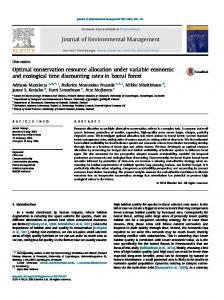
I. I NTRODUCTION In this paper we study a problem of optimally allocating bandwith (or servers) to parallel queues with identically but arbitrarily distributed arrival processes. Special features of this problem are that servers can be assigned in batches, i.e., multiple servers can be allocated to the same queue at a time, and that there is a significant delay between when the allocation decision is made and when the queues are being served, i.e., allocation decision is based on obsolete or delayed state observations. This optimal bandwidth allocation problem is primarily motivated by communication systems that have large propagation delay, e.g., a typical data communication scenario in a satellite network as illustrated in Fig. 1. Users/terminals transmit packets to the Network Operating Center (NOC) via the satellite. The data communication link from users to the satellite, also known as the return channel, follows a dynamic TDMA schedule. Each user is assgined/allocated a certain number of slots within a frame that consists of a fixed number of slots. A user can only transmit within its assigned slots during every frame. A user also inform the NOC of its current queuing situation (e.g., number of backlogged packets) carried either in packet headers or in a special packet at the beginning of its transmission. The assignment/allocation could be determined either by the satellite or by the
2
NOC, and is broadcast to the users over a forward channel, which is separate from (noninterfering with) the return channel. An allocation specifies which slot in the upcoming frame is reserved and to be used by which user. Under such a scenario, due to the long propagation delay of the satellite channel (250 ms from ground/user to satellite and back, or 500 ms from ground/user to ground/NOC via satellite and back), the allocation decision for a particular frame is made based on the backlog information collected during the the previous frame, which is delayed and partially “obsolete” by the time the allocation is used since by that time the backlog situation may have changed. This results in possible over-allocation or under-allocation. Therefore in this case the allocation needs to take into account unknown random arrivals that occur in between observations or state information updates. Satellite
NOC User terminals
Fig. 1. The saatellite communication scenario
Similar resource allocation problems also arise in systems where resource allocation is done relatively infrequently compared to packet transmission time, due to cost or design constraints. In this paper we assume backlogged packets incur a holding cost, and formulate an optimal bandwidth allocation problem for the above scenario, with the objective of minimizing the expected total packet holding cost over a finite time horizon. This objective aims at removing as many packets as possible from the queues since packets remaining in the queue incur a cost. Alternatively it can also be viewed as trying to maximize the total throughput (or utilization) of the channel. We identify two conditions that charaterize a class of allocation policies, and prove their sufficiency for any policy within this class to be optimal given the above objective. In addition, we show that under very mild conditions on the arrival process, these two conditions are also necessary for a policy to be optimal. Without such conditions we show via two examples that in general these two conditions are not necessary for a policy to be optimal. Bandwidth allocation problems have been extensively studied in the literature under various scenarios. Here we review studies most relevant to the one investigated in this paper. Dynamic bandwidth allocation can often be formulated as a dynamic programming problem, the solution of which can always be obtained via numerical methods. However, to obtain a qualitative optimal strategy/policy there is in general no unified framework. The derivation of specific strategies is often highly dependent on the specific scenario under given assumptions. In [1] the problem of parallel queues with different holding cost and a single server was considered, and the simple �� rule was shown to be optimal. [2], [3], [4] considered the server allocation problem to multiple queues with varying connectivity but of the same service class. Each of them determined policies that maximize throughput over
3
an infinite horizon. In particular, [2] derived the sufficient condition for stability and has shown that serving the Longest Connected Queue (LCQ) policy stabilizes the system if system is stablizable. The same policy minimizes the delay in the special case of symmetric queues. [5] further consider a similar problem but with differentiated service classes where different queues have different holding cost, with the objective being to minimize total discounted holding cost over a finite horizon. An interesting result is that the optimality of the index rule holds when the indices are sufficiently separated. All the above considered random connectivity of queues, but the state of the system, i.e., connectivity and the number of packets in each queue, is always known before server allocation is made. In addition it is also commonly assumed that no more than one server can be allocated to a queue at a time. [6], [7] considered the server allocation problem with the assumption that the transmission times are asynchronous. [8] considered the problem of routing arriving packets to a set of queues each having its own server. The structures of these problems are different from the one examined in this paper and they lead to different solutions. Another set of related problems are the bandit problems. The multi-armed bandit problem is concerned with the dynamic allocation of a single server to multiple projects/arms, stated in discrete independent projects/porocesses, where at time the time as follows. Consider a system of state of the system is given. At any time step, we need to activate one of the bandit processes. The activated process will yield a reward as a function of its current state and it will change state according to a Markov process. The goal is to minimize the discounted cost over an infinite horizon. Gittins [9] proved that an index policy is optimal for this problem, where the indices are calculated for each bandit individually as a function of their current states. The optimality of the Gittins index rule has been shown using various techniques, see for example [9], [10], [11], [12]. For a survey see [13] and the references therein. It is shown in [14] that the Gittins index rule is not in general optimal for the case with multiple servers/plays, known as the multi-armed bandit problem with multiple plays. In [15] it is shown that the index policy is optimal under certain conditions on the reward process. �
The problem studied in this paper can be cast as a special case of the restless multi-armed bandit problem [16] with multiple plays, where the passive projects undergo state transitions even when they are not selected. This is because in our case the backlog of each queue continuously change as packets arrive. [16] and [17] studied the asymptotic behavior of this class of problems when the number of arms/projects and servers are infinite with their ratio fixed. Their results do not apply here as the number of queues and servers are finite. A general optimal solution is not known for this class of problems. Our problem is a special case of this class of problems in that 1) The state of the system is not known at the time when the decision is made. This is due to the large propagation delay of the satellite channel; 2) Multiple servers can be assigned to the same project/queue at one decision epoch. That is, the allocation decision not only needs to specify which project/queue to serve (i.e., which queues to assign slots to), but also “how much” it plays/serves (i.e., how many slots to assign to those queues). The rest of the paper is organized as follows. In the next section we describe our network model and formulate the related optimization problem. In Section III we define a class of policies called the residual max-min fair policies and prove their optimality. We also derive conditions on the arrival process under which it is necessary for an optimal policy to be residual max-min fair. In Section IV we show via two examples that in general it is not necessary for an optimal policy to be residual max-min fair. Section V discusses extensions and generalizations of the problem studied here and concludes the paper.
4
II. N ETWORK M ODEL
AND
P ROBLEM F ORMULATION
In this section we describe the network model we adopted as an abstraction of the bandwidth allocation problem described in the previous section, and formally present the optimization problem along with a summary of assumptions and notations. A. The Network Model Consider queues that need to transmit packets to a single server/receiver and compete for shares of a common channel that consists of time slots. Packets arrive at each queue according some abitrary random process. We will assume that queues have identical arrival processes. Packets from these queues are of equal length and one packet transmission time occupies one slot time. The slots ( may or may not be greater than ), i.e., allocation of this channel is done once for assignment is done in batches. These slots together constitute a frame. Within each allocation decision, a queue may be assigned any number of slots not exceeding . An illustration is given in Fig. 2. Alternatively, the above model can also be viewed as one where queues are being served by servers. Different from most of the prior work, here multiple servers can be assigned to a single queue. When this happens, multiple packets will be served. 1
2
Slot assignment Satellite/Server
User/Queues
1
1
2
...... M Slots
N 5
N
Fig. 2. The network model
The allocation decision is based on the backlog information of each queue (number of packets waiting/existing in the queue) provided by the queues at the beginning of a frame. We will ignore the transmission time of such information. This is reasonable since one can always increase the frame length with dedicated fixed number of slots at the beginning for the transmission of such information, which does not affect our discussion of optimal allocation. Based on this information an allocation decision is made by the server/receiver and broadcast to all queues over an non-interfering channel. This broadcast is received by the queues at the end of that frame, in time to be used for the next frame. The same procedure then repeats, which is shown in Fig. 3. Each user advertises its buffer size (denoted by ��� ) to the server. The server allocates slots to be used for transmission in the next time frame, denoted by ����� � . This procedure starts from �
and ends at � �� , the finite time horizon. Note in this scenario during the first frame queues do not have allocated slots and only start transmitting in the second frame (starting � �� ). Similarly, the state information update is not shown for the last frame (starting � ������ ) since the horizon ends at � �� . �
�
�
�
�
We assume that keeping a packet in the buffer at the beginning of a frame incurs a unit cost across all queues. Let ���� be the queue size of queue/user � at the beginning of frame and ��� be �
5 Decision?
b0
Decision?
x1
b1
x2
x_(T−1)
b2
...... 0
1
2
T−1
T
M slots
Fig. 3. The bandwidth allocation dynamics
the slot allocation for that frame. The objective is to find an allocation policy that minimizes the following cost function.
� Where
��
��� ����� � � �� � � � �� �� � � � � �
(1)
summarizes all the information available in the beginning.
B. Assumptions Below we summarize important assumptions underlying our network model. 1) We assume that each user has an infinite buffer size. Without this assumption we need to introduce penalty for packet dropping/blocking. This is an important extension to work reported in this paper and will be considered in a future study. 2) We assume that if the allocated bandwidth for a user is greater than its buffer occupancy (existing backlog carried over from the previous slot) at the beginning of a frame, the newlyarrived packets during that frame cannot be transmitted using the extra slots during that frame. This assumption is essential because the exact arrival times of the packets arriving in a frame is random (e.g., could be toward the beginning of that frame or the end of that frame). Thus whether an extra slot could be used for a new arrival or not depends on the position of the slots in the frame), and the arrival allocated slot (e.g., the first slot or the last slot of the time of the packet. Consequently we will have to take into account different ordering of the allocation (i.e, not only that user � is assigned slots, but also which slots within the frame). This makes the problem very different and much more complicated. In this paper we will limit our attention to the simpler scenario prescribed by this assumption. 3) We assume that all queues have the same arrival process but mutually independent. Arrivals within each frame are mutually independent and also independent of the queue size. Relaxation of this assumption lead the more general model where different users have different arrival processes. This generalization is discussed in more detail in Section V and is currently being invesigated in a separate study. 4) We do not assume that the server knows the arrival process. In other words, the optimal policy does not require the knowledge of the arrival process but it does depend on the fact that queues have identical arrival processes and the previous assumption. 5) We have assumed that all queues have identical holding cost. This precludes differentiation between queues, i.e., all queues are of the same class/priority. Extending this work to consider different service classes is discussed in Section V.
�
�
6
6) The server recalls the latest allocation it has made. Note that the expected cost conditioned on the latest allocation, say � � and buffer occupancy � � is independent of arrivals that occurred before frame , (Note that ��� is a Markov chain with state space � �� �������� where the transition probabilities depend on the control action � � ).
�� for the simplicity of our discussion. 7) We will also adopt the trivial assumption that � It does not affect our results on optimal policy and can be easily relaxed in a straightforward way.
�
C. Notations
We consider time evolution in discrete time steps indexed by � � ������ � , with each increment representing a frame length. Frame refers to the frame defined by the interval
� � . In subsequent discussions we will use terms frames, steps and stages interchangeably. We will also use the terms bandwidth and slots interchangeably. �
�
�
�
�
In general we will use subscripts to denote the time index and the superscripts to denote a specific user/queue. For example � �� denotes the buffer occupancy at the beginning of time slot for the � -th queue. All boldface letters represent column vectors and all normal letters represent scalars. In additionh, if � � ������ �� is an N dimensional vector, then � �� � � . For example ��� is � � an �� � vector representing the number of packets in each queue at time , and � � is a scalar value that represents the total number of packets in all queues at time : � � �� � � �� .
�
� �
�
�
�
��
�
� ��� � �
�
�
Whenever we need to distinguish two policies, we show the policy as a superscript. For example means the buffer size of the � -th queue at time under policy � . �
� � �� ���� ������ � �� ��� : The column vector of all queue occupancies at time . � � �� � � �� � ����� �� �� � � : The number of packet slots (amount of bandwidth) allocated to users. � � �"!$# ��� ��!$# � � , where � % � � takes value % or , ��whichever is greater: The number of pack' ��'
A list of notations are as follows.
���
�
�
�
�
ets in the � -th queue at time (i.e., at the end of the & � � � frame, or the begining of the frame). This value can be completely determined by using the buffer occupancy and allocation information ��' of the & �� � � frame. We will call this amount the existing backlog since this is the amount carried over from the previous slot due to under-allocation (as opposed to new arrivals occurred during the previous frame). Alternatively we will also call this value the amount of deterministic packets to be distinguished from the random arrivals occurred during that frame. �
�
�
�
(
�
*
�
�
frame �� �
+
�
.
: The average number of arrivals during each frame for each queue.
,.-
,.-
� ) �� �) �� ������") �� � � : The number of packet arrivals during frame . � � � � � � � : The excess bandwidth allocated to queue � for random arrivals occurred during �
: The probability of / packet arrivals during a frame for a single queue. Thus 021 )
�4 � . �5 �� � � �
�� 3/ �
�
98 � �;:
�
�76
� � �
5
��
: The cost from time on, or the cost to go. �
� 7< 8 where < 8 is an -dimensional vector with all entries zero except for 1 in the � -the position. � � : The = -fiels induced by all information through time . �
7
III. O PTIMAL P OLICIES In this section we will first establish two conditions that define a class of allocation policies. We will then prove that these two conditions are sufficient for the entire class of policies to be optimal for the objective given in the previous section. In the process of proving this, we will also show that under mild conditions on the arrival process these two conditions are also necessary for a policy to be optimal. A. Preliminaries
� � � ��
�
Claim 1: An optimal policy exists for the problem outlined in the previous section. ! � ! � �
, which is Proof: The total number of policies (possible allocations) is & finite considering a finite horizon � . So the cost function will have a minimum over all possible policies, which means that an optimal policy exists.
�
��
Note that the optimal policy need not be unique. Without loss of generality we assume � The buffer occupancy evolves over time as follows:
� � �� !
� ��
where ) �� !
�
� �
�� ! � � � �
)
�� ! �
.
(2)
is a random variable that represents the arrivals in the interval
� ���� �� �
�
to queue � .
By assumption 3, � �� ! � and ) �� ! � are independent. � � is in general a function of � � �) � �) �� ������ �) � ! � and � �� ������ �� �� ! � . However, by the Markov property of the couple (��� , � � ), the optimum allocation will be a function of only the last state and the last allocation, � �� ! � �� �� ! � . Equation (2) shows that � the buffer occupancy at time consists of two parts, �� � �� ! � � � �� ! � , which is deterministic (meaning that it is known when making the decision �9� ), and a random part ) �� ! � . In subsequent discussions we will call them the deterministic packets and random packets/arrivals, respectively. �� is the information we have available when making a decision for allocation of frame . Thus Equation (2) can be re-written as � �� �� ) �� ! � (3)
�
�
�
�
�
�
Note that we also have # as
� �
�
�
, therefore the cost function to be minimized can also be expressed
������� # ��� �
(4)
From the definition of ��� � given earlier, � � � � � � # are not independent, i.e., given two the third one is uniquely determined. Therefore we have the following result: Remark 1: For any allocation policy we have
� � � � � ��������� � � � � # � � �� ���
(5) The first equality is due to the dependency of � � � � � � # , and the second equality is due to the fact ��������� � � � � � � � � � � � ������� � �
�
�
#
that the expected cost to go is averaged over distribution of � � � # , which is independent of � � given � � # from Equation (3). Following this result, in all our subsequent discussions we will focus on ��� � � � # � rather than ��� � ��� � � � . the conditional cost
� ���
�
� � Definition 1: An allocation �� � � � �������� � �
�����
� � �
����
�
is max-min fair if � � � � for all � . � This defines allocations that result in no queue being allocated more than 2 slots than any other queue. This is essentially the discrete version of the more general max-min fairness. �
8
B. Main Results We define a class of allocation policies
as follows.
Definition 2: If � is a policy that allocates bandwidth to queues such that it satisfies the following two conditions (C-1) all the deterministic packets (or existing backlog) have priority over the random arrivals, i.e. as long as there are known backlog in the queue that have not been scheduled, no slots can be allocated to the unknown, random packets that may or may not be there; (C-2) if there is more bandwidth/slots than the total number of deterministic packets in the system, then the residual bandwidth/slots will be allocated to different queues in a max-min fair manner (i.e. �� � �������� � is max-min fair); then we call � a residual max-min fair (RMF) allocation. We denote by the set of all RMF allocations.
�
Note that strictly speaking our definition of (C-2) implies that (C-1) is satisfied. We state them separately for the ease of our discussions and proofs that follow. Following this definition, we have the following main results of this paper. Theorem 1: Any policy ���� � � minimizes the expected total holding cost given in Equation (1), in that for any other policy � � we have �
� � �� ��� � � � � � �� ��� � �� ��
Theorem 2: Suppose � is an optimal policy that minimizes the expected total holding cost as defined in Equation (1). We have 1) if , � , then � satisfies C-1; 2) if , �� for all � � � , then � also satisfies C-2.
�
� �
Theorem 1 states the sufficient conditions of an optimal policy, the two conditions (C-1) and (C2) outlined above. Theorem 2 states that these conditions are also necessary for an optimal policy if the arrival process satisfies certain conditions, namely that there has to be a non-zero probability of any number, not exceeding � , of packet arrivals during a frame time. (Note that this condition is obviously true in the case of a Poisson arrival process.) From Theorem 1, all ���� are equally optimal, i.e., incur the same cost given the cost function. This means that given the objective function it does not matter whether we favor one queue over another so long as we allocate for all the existing backlog before handling random arrivals. In other words, since the holding cost is identical across all queues and queues are infinite, any backlogged packets, no matter which queue they are in, are equivalent. So serving one or the other does not make a difference. On the other hand, random arrivals have to be treated fairly, i.e., no queue should be more over-allocated than others so as to achieve a balance between queues.
�
In the next subsection we will prove these sufficienct and necessary results through a sequence of lemmas. C. Proof of Optimality In the following lemma we show that under any policy ���� the expected cost depends only on the total number of deterministic packets in the system and not on individual queue sizes.
� ��� � � �
� ��� � � � �
� ��
Lemma 1: Under any given policy ���� , � �� � � � �� � � �� � � & � � for some deterministic function � � � & � � . Moreover, the performance of all policies ���� is the same (i.e. � � � & � �� �� � & � � 4 ���� ).
�
�
9
�
Note that in general, � � & � depends on the set we are averaging on, which is defined by � . However, for convenience we will not emphasize this in notation, unless there is an ambiguity. Proof: We use backward induction on . � + + Induction basis: Let �� , we have � , where is the
� & � expected total arrivals during the last frame. Note that the function does not depend on � . Therefore the induction basis is established. ��� � � � # � ��� � & � �� � Induction step: Suppose – the induction hypothesis. We want to show � �� � � � & � � . � �� � can be written as follows:
� ��� � � � � �
� � � ��
�
�
� ���
� � �� � � � � � � � � �
�
+
5
��
��
� �
�
�
� ��
� �� � � � � �� � � �
����� 5
��
�
�
5 ,
�
��
5 ,
�����
����� �
��
��� �
� ��
� � �
� � � ��
(6)
��'
� � is the arrivals during the & �� � � frame. The first term on the where � &�� � � � right-hand-side (RHS) of (6) is the known backlog in the system at time . The second term is the expected amount of new arrivals by time . The third term is the expected cost to go from time � � ��� � a.s. on, averaged over all possible arrival patterns. Note that � �� � � � By the induction hypothesis we have �
�
�
�
��������� � � �
� ��
� �
�� � ��
�
��� � �
�
�
sum � � &
�
�
� �
� �
�
� � � ���
(7)
% . We now consider two cases, � �� where sum & � � � and � � , respectively. � � Case I ( � � ): In this case under C-1, all assigned slots will be for the deterministic part of � ��� � � � � �76 � � the queues. So sum � � a.s., using Equation (7) we have
�
�
�
�
��������� � � �
� ��
� �
� � �� � � � � � � � ��� � & � � �
Thus we can write equation 6 as follows
� � �� � � � � � � � � �
+
��
5
��
����� 5
�� �
�
5 ,
�
�����
5 ,
� � �� � �
&
�� �
�6 � � � ��
� � �
�6 � � ��
� � �
� � &
� � � ��
(8)
Note that the packets chosen for transmission can be from any queue (or any combination of queues) and this will not affect the expectation of the cost. Therefore all policies satisfying C-1 will have the same performance in this case. Case II ( � � ): In this case all the deterministic packets are assigned slots and possibly (when inequality is strict) some random new arrivals will also be scheduled. Let � �� 1
where 1 and are both non-negative integers and � �� � �� . This is always possible since �& ����� . By (C-2) of the policy ��� 0 slots will be allocated to the random part of each queue according to the following specific rule. users will have 1 � slots assigned and � �� users will have 1 slots assigned. Without loss of generality we will assume that � is a policy that assigns 1 � slots to the first queues and 1 slots to the remaining �� queues. We can then write Equation (6) as follows
� �
�
�
� �.
� � �� ��� � � � � �
+
� ���
� �� &
�
& 1
� � � ��
5
��
�� � � � �
����� 5
�� �
�
� ��� � �
,
5
�
� 1
�����
��
,
5
� � �� � � & � � � �
7�����
�� �
�
� � � �
�
& 1 1
�� �
7�����
(9)
10
if we choose a different policy in that assigns 1 � slots to random queues, not necessarily the first , then by exchanging the sums in Equation (9) we get the same result. Therefore for any other policy in the same expectation will hold, i.e. for all policies satisfying (C-1) and (C-2) the expected cost will be the same. � . Combining the two cases, the induction step is proved. So Lemma 1 holds for all �
� �� �
Definition 3: Define �� & � � � as follows: � � � :
��&
� ����� �
By Lemma 1, for all policies ���
��
� � �� � � �
� � � �
&
�
8
�
�
�! �� �
�
8
�
� � � � � ����� � � � � �
(10)
we have
� � �� � � � � �
�! � �
��
� � &
� � &
� ���
which is independent of � .
�
� � �� � �� & � � � ��
(11)
�
Lemma 2: �� & � � is a positive and non-decreasing function of � almost everywhere, for all under any policy � �� . Proof: We use backward induction on . Again we will omit the superscript � without causing ambiguity. Induction basis: Let � . Then we have
� ���
�
�
� ��� � �
�
8
� � ! �� � �
�
+
����� � � � � ! � � ���
� &� �
��
��
�
So the induction basis is established. Induction step: Assume ��� � & ��� ��� is a positive and non-decreasing function of ��� � . We want to show that ��& � � will also be a positive and non-decreasing function of � . Let’s assume the 8� allocation in the case of � is � � and � � in the case of � under the same policy. Then we have
�
�
� ��� � � �
8
�
�
� ����� � � �
�! �
�
�! �
�
So we can write �� &
��& � � �� �� 5
��
��
+
+
�
��
�
� �.
5
����� 5
�� �
�
5 ,
�
,
�����
5
��
5
��
��
����� 5
��
� � � as follows:
�
�
����� 5
��
�
�
�� �
� �
5 ,
��������� � � � �
�
�
�
5
�����
� 8
,
� ,
����� 5
�
,
5
�
�����
��� �
� ������� � � �
��� � � � � �
�� �
8
� � � � ��� � � �
� ��
� � � � ��������� � � �
� �
�
�
�
) /
��
(12)
�� �
� � � � � ��
� � � �
(13)
� � � � � � ��
(14) We now consider two cases, � and � �� , respectively. Case I ( � ): In this case, by (C-1) of our policy � , all the slots are assigned to the deterministic packets and there will not be any extra slots allocated to random packets. Thus we can write Equation (14) as follows:
� ��
��& � � � �
5
��
��
����� 5
�
�� �
which is positive and non-decreasing in
�
,
5
�
�����
,
5
� ��� � & � ���
� � by the induction hypothesis.
�6 � �� � � � � ��
(15)
11
�
Case II ( � �� ): In this case all the deterministic packets will be scheduled and some random packets will be assigned slots as well. Let � � �1 , where 1 and are non-negative . We further consider two cases and � , respectively. integers and � �� � . By (C-2) of the allocation policy � , Case II.a (
): Since � � , implies 1 we have � �� 1 4 � , i.e. we assign 1 extra slots to all queues for random packets in addition to the deterministic part. When we add one more deterministic packet to the � -th queue, then by (C-1), one of the extra slots must be allocated to this additional packet. Without loss of generality suppose we use one of the extra slots of the first queue, leaving 1 � � extra slots for the first queue. We can then write Equation (14) as follows:
�
�
��& � � �� �
5
�
� ����
5
�� �
����� 5
��
�
�
�
,
5
�
�����
,
5
�
� ��� � & &�� � �
1 �
�� �
�
�� 1
�����
�� � �
1
� � �� ��
(16)
�
Note here we are only summing over � � 1 . This is because for � � � 1 , i.e., the number of new 8� arrivals is below the extra slots assigned, there is no difference between the two scenarios � and 8 � and the corresponding ��� � would be zero. Case II.b ( � ): In this case of the queues (without loss of generality assuming queue � through ) have 1 � slots assigned for their random arrivals and � � queues ( �� through ) have 1 slots assigned for their random arrivals. By (C-2) of policy � , if we have one more deterministic packet, then one of the queues with 1 � slots allocated will have to give up one of its slots (again without loss of generality assuming it is the first queue) for the additional deterministic packet. Thus Equation (14) can be written as follows:
��& � � �
�
5
�
5
��
���� � � � � � � � � & 1 � � � �
����� 5
�
�� �
��
�
,
5
�
� � ���
�����
�� 1
,
5
� ��� � & &�� � �
7�����
�� � �
& 1 1
� �
� 7�����
� � � ��
(17)
Again here we are only summing over ��� 1 � since otherwise there is no difference between 8� 8 the two scenarios � and � . Note that since � � 1 , as � increases, 1 is non-increasing. So by increasing � , the number of elements in the summations in equations (16) and (17) are both non-decreasing. Therefore, using the induction hypothesis that ��� � & � � is positive, we conclude that ��& � � is positive , completing the induction step. and non-decreasing in �
�
�
Corollary 1: � � &
�
�
� �
� � � is a non-negative convex function of � � almost surely for � � �
.
Lemma 1 shows that under a policy in , the expected cost will depend only on the total amount of backlog in the system, i.e., the expected cost to go from time will depend only on the total number of deterministic packets in the system at time , rather than the vector � or # . Using this together with Equation (5) we have �
�
� � �� ����� � � � � � � � �� � � � �� ����� � � �
� #
�
� � � � � �� ����� � � � ��� � � � � ��
(18)
The next two lemmas establish the optimality of (C-1) and (C-2). The first shows that for any policy that does not satisfy (C-1), we can always construct a policy that satisfies (C-1) and results in at most the cost of the original policy. The second shows that for any policy that satisfies (C-1) but does not satisfy (C-2), we can always construct a policy that satisfies (C-2) and results in at most the cost of the original policy.
12
�
�
Lemma 3: Suppose a policy � violates (C-1), then there exists a policy � such that � does not � violate (C-1) and � a.s., moreover, if , � , the inequality is strict. � Proof: Suppose � violates (C-1) in some frame , some queue must be under-allocated (i.e., not all deterministic packets are assigned slots) and some queue must be over-allocated (i.e., extra slots are assigned for random arrivals). Therefore under � there exist � such that ���� � �� and � � � � . We construct a policy � as follows. � is the same as � up to frame . Therefore cost incurred upto and including time under � and � is the same. At time frame , let � �� � �� � and � � � � � � be the allocation under � for � , respectively. In words, we re-allocate one of the slots reserved for queue ’s random arrivals to queue � ’s existing backlog, and keep everything else the same. Under policy � there are � � 3� � � � slots reserved for random arrivals at queue . Under policy � we denote by � � � � � � � � the amount reserved for random arrivals at queue . From this point on two situations are possible. Consider the first case where the number of arrivals to queue during the �� � -th time frame ( ) � ! � ) is less than � � � � , i.e., ) � ! � ��� � , then � and � result in the same backlog in queue at time � � since both allocations assign more than necessary. As a result, under � we will have one less backlogged packet in queue � at time � , 8� while all other queues have the same backlog compared to that under policy � . That is, � � #
� � # a.s., where is the backlog for policy � . Therefore at time � , cost under � is one more than cost under � . For the remaining frames, we let � give the exact same allocation � � � # ������ � !$# as given by � , thus incurring at most the same cost to go as that under � . � � � Now consider the second case where ) � ! � � . Under policy � , at � we have one packet more in queue and one packet less in queue � compared to that under policy � . Thus cost incurred up to and including 9 � is the same for both policies. At 9 � , we will let � assign one more slot to queue and one less to � compared to that given by � , which then results in the exact same backlog situation at time 7� . From this point on, � will give the exact same allocation as that given by � , incurring the same cost to go as that under � . Combining the above two cases, we have constructed a policy � , that incurs at most the cost as incurred by � , expressed as follows:
� ����� � � � � ����� � �
�
� �� � �
�
�
�
�
�
�
�
� � �� � ��
�
�
�
�
�
�
� �� �
�
�
�
�
�
�
�
� � � ��
�
�
�
�
�
�
�
�� � � �� � � � ����� � � � � ! � � , & ) �� ! � � � �� � � �� � � � ����� � � � � ! � � � , & ) �� ! � � � �� � � �� ��& � � ����� � � � � ! � � � � � , & ) �� ! � � � �� � � �� � � � ����� � � � � ! � �
� � ��� � � � � � ! � � � , & ) �� ! � � � �� � � �� � � � � ����� � � � � ! � � Where all the equalities and inequalities hold almost surely. � � � � � Note that the last inequality becomes strict if , & ) � ! � � � � � � � � is positive. Since � � ��� � � ,
� � �� ��� � � � �
�! �
�
,
& )
�� !
� �
�
�
�
it suffices to have , � in order for the strict inequality to hold. Since the cost upto is the same , under both policies, we have � 2� � , the inequality # # � �) / . Moreover, if is strict. � Starting from any policy � that does not satisfy (C-1), we can construct a policy � by repeatedly using the same construction outlined above. More specifically, starting from the first time when (C1) is violated under � , we can construct a policy that assigns more slots to deterministic packets compared to � and results in at most the cost of � . Repeating for a finite number of times we will obtain a policy that satisfies (C-1) at this time frame. We then move on to the next time when (C-1)� is violated and so on. Repeating this procedure for a finite number of times, we obtain a policy � � that results in at most the cost of policy � and does not violate (C-1). Moreover, if , � , then � is strictly better than � .
� ��� � � � � � ����� �
� �
�
13
�
Lemma 4: For a policy � � that satisfies (C-1) but not (C-2), there exists a policy � that satisfies both (C-1) and (C-2), and � a.s. � Proof: We use backward induction on the time when (C-2) is violated under � to show that we can always find a policy that satisfies (C-2) with no increased cost for � ���� � � � � ������ � . Induction basis: Suppose � is not residual max-min fair in the last step, i.e., there exist � such � ! � � . We show that if we subtract one from � � ! � and add one to user � ! � , that, � � ! � the expected cost will be no more under the new allocation. Define policy � to be the same as � up to time frame � � � . At � � � let � � ! � � � ! � � � and � ! � �� ! � � be the allocation for � �
� . random arrivals under � for � , respectively. For all the other queues set � ! � � ! � Since the cost incurred in all the previous time frames remain the same we only need to consider the expected cost for the last frame � � � . Since the allocation for all the other queues except � is the same, the expected queue sizes for those queues remain the same. Thus we only need to consider the difference between the sum of the expected values of queues � under these two policies:
� ����� � � � � ��� � � �
�
� ��
�
�
�
�
�
��
�
��
�
� � �
�
�
�
� � � ����� � � � � � �� � � � � �& � � � � �� � � � � � �� � ��� & � � � � �� � � � � � �� � �� ��
+ � � ) �� � �� a.s.and by definition, � �� � � �� ! � � � �� ! � � We have � � � �� � � � ! � �
! �
�
�
(19) �
Under policy � we have (using / to represent the number of arrivals during frame ��� � ):
� � � � �� �
+
� � � � �� �
+
Under policy � we have:
� � � � �� �
+
� � � � �� �
+
�
�
��
�
-
� � �
/ �
� �
/ �
-
,
��
�
-
� � �
/ �
� �
/ �
�� � ��� � -
� � ��� �
-
�
,
-
�
&
� � � � �� � � � � � � � � � �
&
��� � � -
�� �
�
��� � � -
��
,
+
+
Using the above equations we get:
� � � � �� � � � � � �� � ��
�
,����
��
�
-
-
� � �
/ �
� �
/ �
,
,
�� � ��� �
�
-
� �
!
,
�
�� ! � � � �
.
�� � �
��
� � - ��� � � �
� ��� � ! � �� � ! � � �
�
-
�
��� � � -
�
��
(20)
which means that the expected cost for policy � is at most the expected cost for policy � . It is also clear from the above expression that if , � ��� � � � � then the inequality is strict. � may or may not be residual max-min fair at time � � � , but � is “closer” to� being RMF than � . If we repeat this procedure a finite number of times we can obtain a policy � that satisfies (C-2) at time � ��� and results in at most the cost incurred by � . Induction basis is thus established. Induction step: Now assume that � satisfies (C-2) for all time frames 9 � � ������ � � � , but violates (C-2) at . This means that there exists � such that � � � � � � . Define policy � to be the same as � up to time . At time we let � �� � �� � � and � � � � � , i.e., subtract one slot from queue � and allocate it to queue . Thus � � � �� � � ��� and � � �� � � . Starting � , both policies satisfy (C-2). We show that policy � incurs at most the cost incurred by policy � .
�
�
�
�
�
�
�
�
�� �
�
�
�
14
Since the policies are the same for all frames before , we only need to consider the cost to go ��� � � . The number of deterministic packets in the queues at time , � , serves as from on, an initial condition. Since from frame 9 � on (C-2) is satisfied, by Lemma 1 the expected cost of all those frames will only depend on the sum of all the packets in the system. We have
�����
�
�� �
�
�
�
� � ����� � � � � � ��� � � �
� � ����� � � ! � � � � � ���� � � � ! � �
�
��
�
5
��
�
� �
�
����� 5
��
5 ,
�
�����
� � ������� � � � �� � �
�
�
5 ,
� � �� ����� � � � ��� � �
�
sum &
� ��� ��
� ��
��'
�
sum & �
� ��
� �
�� � � �� �
� � � � ��
(21)
where � � ������ � is the arrival to the queues during the & � � � frame. We now partition all the possible transitions from step � � to step as follows. The probability that we have � new 5 5 � arrivals in queue � and � new arrivals in queue during frame � � is , � , . We partition all pairs &�� � � � � � into the following four sets: � � � &�� � � � � � � ��� � � � � � � ;
&�� � � � � � � �� � � ��� � � � ; ���
&�� � � � � � ��� ��� � � � � � � ; ��
&�� � � � � � ��� �� � � ��� � � � . �� � and &�� � � � � , the sum of deterministic packets in queues � is For all pairs &�� � � � � the same under both policies � and � since � results in under-allocation under both policies, and � results in over-allocation under both policies. For all pairs &�� � � � the sum of deterministic � � �� packets under policy � is one more than that under policy � . For all pairs &�� � � � the situation � is the opposite. 5 5 � �� to denote summing over all possible arrivals For simplicity, we will use the notation � � to all queues such that &�� � � � . Using this notation, Equation (21) can be written as �
� � � �
� � �
� � �
� �
� �
��
�
�� � �� � �� � �� ��
�
5
�
� � 5
�
�
5
�
,
5
� � � �
5
�
5
5
�
,
�����
5
�
�
5
�
5
�
� � �� �
,
5
,
�
�����
,
�
�
�
�
�
However, note that �
�
�
�����
� � �� ����� � � � ��� � � � � � � � � � � � � ������� � � � ��� � � � � & � �� ��� � �� � � � � � ��� � 5 5 � , , � 5 � � 5 � � �� � ����� � � � � ��� ��� � � � ��� � � � � � � ������� � � � ��� � � � � & � �� � � �� � � � � � ��� �
�
�
�
�
�
� ��� �
�
�
� � � � ����� # � �� � � � � �� ��� # � � �
&��
�
�
��� ��
� �� �
�
� ��� �� � � �
�
��
���
Define the set � to be �
�
�
&��
� �
� � � &���� � � � �
�
�
��
�
�
&��
5 ,
�
��� ��
��
�
��� �� �
� � � � �
�
�
���
� ��
�� �
� �
��
�� �
� �
��
�
�
���
��� �
� � � �� ��
�
(22)
(23)
15
�� �
and we have
following Equation (23). Equation (21) can thus be written as
�
� � �� ��� # � � � � � � �� ��� # � � �
�
�
�
5
5
5 ,
�
� �
�
�
�
� � �� ����� � � � ��� � �
�
��� � � � ��� �
� � �� �
� � �� ����� � � � ��� � � , �
�
�
5
5
�
� � �� !
�
5
��
� � �� ����� � � � ��� � �
,
�����
�
�
5
�
��� � � � �� � � � � ��� �� �� � � � � � � ��� � �� � � � � � & � �� ��� � �� � � � � � ��� � �� � � � � � ��� � �� � � � � � � ��� � ��� � � � � & � �� � � �� � � � � � � �� � �� � 5 � � �� � � � � � � , � ����� � � � ������� � � � ��� � � � ��� � � � ��� � � � � � & � �� � � � � � � � � � � � ��
(24) ��� � ��� �
�
� � �� �
Thus we have
� � � �� ��� # � 5 � � � � 5 � �� ��� # � � � , � , �
�
�
5
5
� � 5
� �
�
�
5
�
�
� � �� !
�
����� ,
��
��� � &�� � �
5
�
�
�����
5 ,
�
��
& �
��� � &�� � � �
� � & �
��
�
�
� � � � � � � � � ��� � &�� � �� � ��� � � � � � � � � � � � �
��� � � ���
��� ��
�
���
��� �
�� �
��
� �
(25) �
Note that we have left out the superscripts � and � in ��� � & � � . This is because both � and � satisfy (C-1) and (C-2) from time � on by the induction hypothesis, and are thus indistinguishable given the initial condition ��� � . Using Lemma 2 and Corollary 1, the first term in Equation (25) is nonnegative due to the convexity of ��� � & � � and the assumption � � � � � � � . The second term is also non-negative since ��� � & � � is positive by Lemma 2. Thus we have shown that � incurs at most the cost incurred by � , and similar to the induction basis, � is “closer” to� being RMF than � . If we repeat this procedure a finite number of times we can obtain a policy � that satisfies (C-2) at time and results in at most the cost incurred by � . The induction step is thus proved. Therefore for any policy � that satisfies �(C-1) but not (C-2) we can use the above procedure going backwards in time to construct a policy � that satisfies (C-2) and has a cost of at most that incurred by � .
�
�
�
�
�
Note that in the above proof
� � �
that
��
�
� �
&��
�
� ���
�
because �
� �� � �
�
� � ��
��
� � � � �
�
. Indeed it can be easily verified
��� �� �
Thus if , � � � � � , then the second term in Equation (25) is guaranteed to be strictly positive. In this case policy � is strictly better than policy � . This leads to the following corollary. �
� �
,
� , then a residual Corollary 2: If the � arrival� process has the property that � � for all � � max-min fair policy � (i.e., � satisfies (C-2)) is strictly better than one that violates (C-2). Proof: First note that if under a certain policy we have � � �
� for all � and , then this policy is residual max-min fair. Suppose policy � violates (C-2) in some time frame , then there exist � such that � �� � � � and � � � � . We know that , � � � � will guarantee Equation (25) to
� �
�
�
� �
�
�
�
� �
�
16
be strictly positive, i.e., , � �
� �
�
means that we can find a policy that is strictly better than � . By
� �
repeating the procedure� used in Lemma 4, , � for all �
� means that we can find a residual � max-min fair policy � that is strictly better than any � that is not residual max-min fair. This in turns shows that given the property , �� for all �
� , an optimal policy is necessarily residual � max-min fair, i.e., an optimal policy has to satisfy (C-2).
�� �
This corollary implies that if the arrival process has the property , (C-2) or residual max-min fair is necessary for a policy to be optimal.
�
�
for all
�
� � � , then
Combining Lemmas 3 and 4 we obtain Theorem 1. Lemma 3 and Corollary 2 lead to Theorem 2. IV. S UFFICIENT B UT N OT N ECESSARY – T WO E XAMPLES In the previous section, we proved that any policy � � minimizes the cost function and therefore is optimal. However, under certain conditions on the arrival process there may be other policies that are not residual max-min fair, but are nevertheless optimal. In other words, (C-1) and (C-2) are not in general necessary for a policy to be optimal. We derived two assumptions on the arrival process under which (C-1) and (C-2) become necessary for optimality. In this section we provide two examples to illustrate that without these assumptions on the arrival process, an optimal policy need not be residual max-min fair. Example 1: Consider two users ( � ) and a time horizon � � (i.e. the only time an
��
�"� � . Suppose the arrival process is a allocation is made is at � ). Let � weighted poisson process, where all probabilities are weighted by . Thus all probabilities ,$- are � , ,
or � . equal to the pmf of a poisson process conditioned on A residual max-min fair policy would assign slots to all the deterministic packets and not allocate �� . However, one can easily check that any other policy any slots for random arrivals, i.e. �
that allocates one slot to the random arrivals for one queue and the rest of the slots to deterministic � will both have the packets will have the same expected cost. For example � � and �
same expected cost as the RMF policy, although they do not satisfy (C-1). This is due to the fact that the probability of having no arrival in a frame is zero, with the weighted poisson process.
� ��
�
��� �
���
� �� �
� � �
Example 2: Consider two users ( � ) and a time horizon � � . Let , �
, � , and , � . A residual max-min fair policy is to let � queue allocate one slot for random arrivals). Thus we have
� ����� � � � � �� � � � � � � �� � � � �
��
�� �
�
� �� �
�
� &
�
� �
� &
�
��� � � � � (i.e � for �each
� � �
�
�
��
� �
Now suppose we have an allocation � � . It can be easily shown that under this policy the expected cost is also , although this allocation violates (C-2) and thus is not residual max-min fair.
V. D ISCUSSION
AND
C ONCLUSION
The main result obtained in the previous sections are highly intuitive. In essence, since queues are infinite and the only cost is packet holding cost, we should clear up the existing packets as quickly as possible in order to minimize the total cost. (C-1) implies that due to the delay of state information, we don’t know for sure how many new arrivals are in the system. Therefore so long as there are known backlog in the system that need to be allocated, we should never allocate for a new arrival that may or may not be there. Since holding cost is constant and identical for all queues, all
17
existing backlog become equivalent. Consequently it does not matter which queue we serve first and for how much so long as we serve the deterministic backlog first. (C-2) implies that if we have to allocate for the unknown part of the queue, the best things to do is to allocate them fairly among all queues. This prevents any particular queue from becoming too large and incur extra holding cost. It is worth mentioning that we could also discount the cost over time and define
�
�� �� � �
�
�� � �� �� �
where � � is the discount factor. All our lemmas and theorems still hold in this case with simple modifications to the proofs. Below we discuss some interesting and important extensions and generalizations of the problem studied here, by relaxing some of the assumptions we have made. These are part of our on-going study. (Assumption 1): An important extension is to drop the infinite queue assumption, and to place a penalty on dropping/blocking packets. Intuitively, the longest queue first type of policy should be optimal in this case. Note that longest queue first policy is a subset of defined by (C-1) and (C-2). (Assumption 3): If arrival processes are different for different queues, then (C-1) should still hold given the holding costs are the same. (C-2) no longer holds. Instead the allocation for random arrivals may be some form of weighted max-min fair taking into account different arrival processes. (Assumption 5): Another interesting extension is to account for differentiated service classes represented by different holding costs, as considered in [5]. The objective is again to minimize the total expected holding cost, or the weighted sum of number of packets in the system weighted by different holding costs. Higher packet holding cost implies a higher-priority queue. In this case the allocation will have to take the arrival process into account. (Note that for the problem studied in this paper we do not need arrival statistics to determine the optimal allocation, under the assumption that all arrivals are identically distributed). We conjecture that some type of index policy may be optimal in this case. Similarly we could consider queue connectivity probabilities and the probability of packet transmission success/failure. One may also consider the total expected discounted holding cost over an infinite horizon as the objective function to be minimized. Although not immediately obvious from the proofs shown here, our conjecture is that the same set of policies will still be optimal for the infinite horizon case. To conclude, in this paper we considered the problem of finding an optimal policy to minimize the total number of packets/jobs in the system over a finite horizon. The features of this problem include (1) there is a large delay between when the allocation decision is made and when the allocation is used, thus decisions can be viewed as based on delayed or obsolete state information/observations; and (2) the bandwidth allocation is in frames of time slots so that each queue can be assigned any number of slots not exceeding the total number in a frame. We established two conditions under which a policy will be optimal. These two conditions define a set of policies among all admissible policies. We also argued that in general these conditions need not be necessary for the optimality of a policy. We proved that under some mild conditions on the arrival process, these two conditions are also necessary for the optimality of a policy.
18
R EFERENCES [1] C. Buyukkoc, P. Varaiya, and J. Warland, “The �� -rule revisited,” Advances in Applied Probability, vol. 17, pp. 237–238, 1985. [2] L. Tassiulas and A. Ephremides, “Dynamic server allocation to parallel queues with randomly varying connectivity,” IEEE Transactions on Information Theory, vol. 39, no. 2, pp. 466–478, March 1993. [3] L. Tassiulas, “Scheduling and performance limits of networks with constantly changing topology,” IEEE Transactions on Information Theory, vol. 43, no. 3, pp. 1067–73, May 1997. [4] N. Bambos and G. Michailidis, “On the stationary dynamics of parallel queues with random server connectivities,” Proc. 43th Conference on Decision and Control (CDC), pp. 3638–43, 1995, New Orleans, LA. [5] C. Lott and D. Teneketzis, “On the optimality of an index rule in multi-channel allocation for single-hop mobile networks with multiple service classes,” Probability in the Engineering and Informational Sciences, vol. 14, no. 3, pp. 259–297, July 2000. [6] L. Tassiulas and S. Papavassiliou, “Optimal anticipative scheduling with asynchronous transmission opportunities,” IEEE Transactions on Automatic Control, vol. 40, no. 12, pp. 2052–62, December 1995. [7] M. Carr and B. Hajek, “Scheduling with asynchronous service opportunities with applications to multiple satellite systems,” IEEE Transactions on Automatic Control, vol. 38, no. 12, pp. 1820–33, December 1993. [8] P. Sparaggis, D. Towsley, and C. Cassandras, “Extremal properties of the shortest/longest non-full queue policies in finite-capacity systems with state-dependent service rates,” Journal of Applied Probability, vol. 30, pp. 233–236, 1993. [9] J. C. Gittins, “Bandit processes and dynamic allocation indices,” J. Royal Statistical Society Series, vol. B14, pp. 148–167, 1972. [10] R. R. Weber, “On the gittins index for multi-armed bandits,” The Annals of Applied Probability, vol. 2, pp. 1024– 1033, 1994. [11] P. Whittle, “Multi-armed bandits and the gittins index,” Journal of the Royal Statistical Society, vol. 42, no. 2, pp. 143–149, 1980. [12] D. Bertsimas and J. Nino-Mora, “Conversion laws, extended polymatroids and multi-armed bandit problems,” Mathematics of Operations Research, vol. 21, pp. 257–306, 1996. [13] E. Frostig and G. Weiss, “Four proofs of gittins’ multi-armed bandit theorem,” Applied Probability Trust, November 1999. [14] T. Ishikida, “Informational aspects of decentralized resource allocation,” PhD. Thesis, University of California, Berkeley, 1992. [15] D. G. Pandelis and D. Teneketzis, “On the optimality of the gittins index rule for multi-armed bandits with multiple plays,” Mathematical Methods of Operations Research, vol. 50, pp. 449–461, 1990. [16] P. Whittle, “Restless bandits: Activity allocation in a changing world,” A Celebration of Applied Probability, ed. J. Gani, Journal of applied probability, vol. 25A, pp. 287–298, 1988. [17] R. Weber and G. Weiss, “On an index policy for restless bandits,” Journal of Applied Probability, vol. 27, pp. 637–648, 1990.