Optimal Control for Discrete Event and Hybrid Systems∗

Optimal Control for Discrete Event and Hybrid Systems∗ Christos G. Cassandras and Kagan Gokbayrak Dept. of Manufacturing Engineering Boston University Boston, MA Dedicated to Yu-Chi (Larry) Ho

Abstract As time-driven and event-driven systems are rapidly coming together, the field of optimal control is presented with an opportunity to expand its horizons to these new “hybrid” dynamic systems. In this paper, we consider a general optimal control problem formulation for such systems and describe a modeling framework allowing us to decompose the problem into lower and higher-level components. We then show how to apply this setting to a class of switched linear systems with a simple event-driven switching process, in which case explicit solutions may often be obtained. For a different class of problems, where the complexity lies in the nondifferentiable nature of event-driven dynamics, we show that a different type of decomposition still allows us to obtain explicit solutions for a class of such problems. These two classes of problems illustrate the differences between various sources of complexity that one needs to confront in tackling optimal control problems for discrete-event and hybrid systems.

1

Introduction

The theory and extensive applications of optimal control for dynamic systems are documented in several books, including “Applied Optimal Control” [1], co-authored by Bryson and Ho. Since this paper, along with the rest in this collection, is dedicated to the second author, it is most appropriate that its topic covers two areas to which Larry Ho has made fundamental contributions: optimal control and discrete event systems. The emergence of hybrid systems, which has largely motivated the work presented here, arguably owes its rapid growth to the foundations laid by the development of modeling frameworks and analytical techniques for discrete event systems. ∗

This material is based on work supported in part by the National Science Foundation under Grants ACI-9873339 and EEC-00-88073, by AFOSR under contract F49620-01-0056, and by the Air Force Research Laboratory under contract F30602-99-C-0057.

1

Optimal control methodologies have been based on a modeling framework for dynamic systems which revolves around the differential equation x˙ = f (x, u, t)

(1)

describing the dynamics of a system whose state at time t is captured by a vector x(t) and whose behavior is dependent upon some input or control vector u(t). We refer to this class of systems as time-driven because their state continuously changes as time evolves. Typical examples include mechanical systems whose state consists of variables representing physical position and velocity, or chemical systems whose state includes the temperature or pressure for certain physical processes. In contrast, Discrete Event Systems (DES) are characterized by eventdriven dynamics. In this case, state variables are usually discrete and change only as a result of the occurrence of events; they do not continuously change over time. One encounters DES in modern technological settings such as automated manufacturing, communication networks, and computer operating systems. As an example, let x(t) be the number of packets waiting in a buffer to be processed by some network switch at time t. The only way this quantity can change is if a packet is removed from the buffer and transmitted (in which case the state changes by −1) or if a new packet is added to the buffer (in which case the state changes by +1). Both changes occur instantaneously when the event “packet processed” or the event “new packet arrives” respectively takes place. Clearly, (1) is neither natural nor appropriate for describing the dynamics of such an event-driven system: the state in between events is unchanged and the derivative of x(t) is not defined at event times (at least not in a strict sense that can make it useful for analysis purposes). Modeling frameworks for DES were developed over the 1980s along several different directions, including untimed and timed automata and Petri nets (for a comprehensive overview, see [2]). Because these modeling frameworks are drastically different form (1), optimal control methodologies developed on the basis of time-driven dynamics are simply not transferable to the DES setting, although fundamental principles (e.g., dynamic programming) obviously still apply. To complicate matters, many interesting optimal control problems one encounters in DES involve some form of uncertainty (e.g., in the example of a packet buffer, the processes that describe arrival and processing events are generally stochastic); this implies that ideas and techniques from stochastic optimal control need to be invoked. The advent of hybrid systems makes the development of optimal control beyond classical timedriven systems an even greater challenge. The term “hybrid” is used to characterize systems that combine time-driven and event-driven dynamics. Broadly speaking, two categories of modeling frameworks have been proposed to study hybrid systems: Those that extend event-driven models to include time-driven dynamics; and those that extend the traditional time-driven models to include event-driven dynamics; for an overview, see [3]. A simple way to think of a hybrid system is as one characterized by a set of operating “modes”, each one evolving according to time-driven dynamics of the form (1). The system switches between modes through discrete events which may be controlled or uncontrolled. Controlling the switching times, when possible, and choosing among several feasible modes, whenever such choices are available, gives rise to a rich class of optimal control problems. This has motivated efforts to extend classical optimal control principles [4],[5],[6] and to apply dynamic programming techniques [7],[8]. While in principle this is possible, the computational complexity involved becomes prohibitive: not only does one have to deal with the well-known “curse of dimensionality” in such problems, but there are at least two additional sources of complexity to deal with, i.e., the presence of switching 2

events causing transitions from one mode to another (which introduces a combinatorial element into the control), and the presence of event-driven dynamics for the switching times (which introduce nondifferentiabilities). Therefore, keys to the successful development of optimal control methods for hybrid systems are: (i ) seeking structural properties that allow the decomposition of such systems into simpler components, and (ii) making use of efficient numerical techniques. Along these lines, progress has been reported for classes of hybrid systems whose structure may be exploited. For example, in [9] a Mixed Logical Dynamical (MLD) system framework is proposed, which allows the use of efficient methods developed for piecewise affine systems, and in [10] optimal controllers are presented for the class of autonomous switched linear systems. The hybrid system modeling framework we consider in this paper is motivated by the fact that it is often natural to hierarchically decompose systems into a lower-level component representing physical processes characterized by time-driven dynamics and a higher-level component representing discrete events related to these physical processes (e.g., switching from one mode of operation to another, as in shifting gears in an automotive system). Our objective is to formulate and solve optimal control problems associated with trade-offs between the operation of physical processes and timing issues related to the overall performance of the system. For a class of such optimal control problems, a hierarchical decomposition method was introduced in [11]. This method enables us to design a controller which has the task of communicating with both components and jointly solving coupled optimization problems, one for each component. The same basic idea is also independently proposed in [12]. The explicit solution of the lower and higher-level problems depends on the specifics of the time-driven and event-driven dynamics involved. In the remainder of this paper, we first describe a convenient modeling framework for hybrid systems allowing us to decompose them into lower (time-driven) and higher (event—driven) level components. Subsequently, we formulate an optimal control problem and present a solution approach based on this decomposition. In Section 3 we describe how to apply this setting to a class of hybrid systems where all operating modes have linear time-driven dynamics and the event-driven switching process is very simple. In this case, we find that the hierarchical decomposition approach requires solving a nonlinear parametric optimization problem coupled with a number of standard optimal control problems subject to purely time-driven dynamics; explicit solutions of such problems are occasionally possible, as illustrated by an example. In Section 4, we consider a different class of problems where the complexity lies in the eventdriven dynamics which are nondifferentiable. In this case, we show that a different type of decomposition allows us to obtain explicit solutions for a class of such problems. While the approaches presented for solving these two classes of problems help to lay the foundations for extending classical optimal control theory, they also serve to identify the differences between various sources of complexity that one needs to understand and address in order to handle the challenges of new technological environments where these complexities manifest themselves.

3

2

Optimal Control Problem Formulation

In the hybrid systems we consider, the state of the system consists of temporal and physical components. The temporal components keep track of the time information for events that may cause switches in the operating mode of the system. Let i = 1, 2, . . . index these events. We denote the physical state of the system after the ith event by zi (t) with dynamics: z˙i = gi (zi , ui , t),

zi (xi−1 ) = zi0 ,

t ∈ [xi−1 , xi )

(2)

where ui is the control applied over an interval [xi−1 , xi ) defined by two event occurrences at times xi−1 and xi . In what follows, we shall write ui to denote a function ui (t) defined over [xi−1 , xi ); similarly for zi (t). We shall assume that ui (t) is allowed to be piecewise continuous and is in general an n-dimensional vector. In the case of a single event process in the system, the event-driven dynamics characterizing the temporal states xi are given by (3) xi = xi−1 + γi (zi , ui ) for i = 1, 2, . . ., where γi (·) represents the amount of time between switches, which generally depends on the physical state zi and control ui over [xi−1 , xi ). In the case of multiple asynchronous event processes in the system indexed by j = 1, . . . , M , we need to introduce a Timed Automaton which determines which of the M events in the system triggers the next switch and at what precise time. The exact structure of a timed automaton is described in [2]. We limit ourselves here to a brief review of its definition and basic operation. An Automaton, denoted by G, is a five-tuple G = (Q, E, f, Γ, x0 ) where Q is the set of states; E is the finite set of events associated with the transitions in G; f : Q × E → Q is the transition function, where f (q, e) = r means that there is a transition labeled by event e from state q to state r (in general, f is a partial function on its domain); Γ : Q → 2E is the active event function (or feasible event function), where Γ(q) is the set of all events e for which f (q, e) is defined and it is called the active event set (or feasible event set) of G at q; and q0 is the initial state. The automaton G operates as follows. It starts in the initial state q0 and upon the occurrence of an event e ∈ Γ(q0 ) ⊆ E it makes a transition to state f (q0 , e) ∈ Q. This process then continues based on the transitions for which f is defined. Note that an event may occur without changing the state, i.e., it is possible that f (q, e) = q. As it stands, this model is based on the premise that a given event sequence {e1 , e2 , . . .} is provided, so that, starting at state q0 , we can generate a state sequence {q0 , f (q0 , e1 ), f (f (q0 , e1 ), e2 ), . . .}. We extend our modeling setting to Timed automata by incorporating a Clock Structure associated with the event set E which now becomes the input from which a specific event sequence can be deduced. This clock structure is a set V = {vi : i ∈ E} of clock (or lifetime) sequences vi = {vi,1 , vi,2 , . . .}, i ∈ E, vi,k ∈ R+ , k = 1, 2, . . . With this in mind, the original automaton now becomes a six-tuple (Q, E, f, Γ, x0 , V) where V = {vi : i ∈ E} is a clock structure. The timed automaton generates a state sequence q 0 = f (q, e0 ) 4

(4)

driven by an event sequence {e1 , e2 , . . .} generated through e0 = arg min {yi }

(5)

i∈Γ(q)

with the clock values yi , i ∈ E, defined by ½ yi − y ∗ if i 6= e0 and i ∈ Γ(q) 0 yi = / Γ(q) vi,Ni +1 if i = e0 or i ∈

i ∈ Γ(q 0 )

(6)

where the interevent time y ∗ is defined as y ∗ = min {yi }

(7)

i∈Γ(q)

and the event scores Ni , i ∈ E, are defined by ½ Ni + 1 if i = e0 or i ∈ / Γ(q) 0 Ni = otherwise Ni

i ∈ Γ(q 0 )

(8)

/ Γ(q0 ), then yi In addition, initial conditions are: yi = vi,1 and Ni = 1 for all i ∈ Γ(q0 ). If i ∈ is undefined and Ni = 0. In this setting, the clock structure V is assumed to be fully specified in a deterministic sense. A Stochastic Timed Automaton is obtained when the clock sequences are specified only as stochastic sequences {Vi,k } = {Vi,1 , Vi,2 , . . .}, in which case each {Vi,k } is characterized by a distribution function Gi (t) = P [Vi ≤ t]. In the sequel, the details of the timed automaton that controls the mode switches are not required and are suppressed by simply representing the event-driven dynamics in the form xi = xi−1 + γi (yi,1 , . . . , yi,M , zi , ui )

(9)

where yi,1 , . . . , yi,M are the event clocks of the timed automaton (through which the triggering event and its occurrence time for the next switch are determined) after the (i − 1)th switch. We note, that γi (·) above generally involves the min operation seen in (5), introducing nondifferentiabilities which can significantly complicate the analysis. Looking at (2) and (9), note also that the choice of control ui affects both the physical state zi and the temporal state xi . Thus, the switches at times x1 , x2, . . . are generally not exogenous events that dictate changes in the state dynamics, but rather temporal states intrically connected to the control of the system; this is one of the crucial elements of a “hybrid” system. The optimal control problem we now consider has the general form min J = u

N X

[φi (xi−1 , xi ) + ψi (xi )]

(10)

i=1

subject to (2) and (9), where    u1 (t) u = ...   uN (t)

t ∈ [x0 , x1 ) .. . t ∈ [xN−1 , xN ) 5

(11)

The function φi (xi , xi−1 ) is the cost of operating the system with control ui over the interval [xi−1 , xi ), which results in the physical state {zi (t), t ∈ [xi−1 , xi )}. This is generally expressed as Z xi f φi (xi−1 , xi ) = h(zi ) + Li (zi (t), ui (t))dt xi−1

h(zif )

where is a terminal cost associated with the physical state zif = zi (xi ) and Li (zi (t), ui (t)) is a cost function dependent on the physical state and control during the ith mode. Note that φi (·) is expressed as a function of the starting and ending times for the ith mode, but it obviously depends on the choice of control used over [xi−1 , xi ). The function ψi (xi ) is the cost associated with the occurrence time xi of the ith event. The intent is to penalize switching times that occur later rather than earlier, which creates a trade-off with the requirement that a certain desired physical state zi (xi ) be attained, which may not be possible if xi is too short. In (10), the time horizon is determined by a given number of switches N and the control does not include selecting the next mode. Thus, it is assumed that the sequence of modes to be used is prespecified (e.g., as in changing gears in an automobile). Moreover, note that in this formulation the only control is u, through which the physical and tempoiral states are affected. In some variations of this problem, it is possible that the switching times x1 , . . . , xN may be exogenous controllable variables as well. Let si = xi − xi−1 ≥ 0, i = 1, 2, . . . Assuming stationarity of the cost φi (·) in the sense that φi (xi−1 , xi−1 + si ) = φi (0, si ) ≡ φi (si ), we can write Z si Li (zi (t), ui (t))dt (12) φi (si ) = h(zif ) + 0

Thus, the optimal control problem we consider can be written as min J = u

N X

[φi (si ) + ψi (xi )]

(13)

i=1

subject to (2) and (9) with u as defined in (11) and φi (si ) as defined in (12).

2.1

Hierarchical Decomposition

Consider an interval [xi−1 , xi ) and suppose the initial and final physical states, zi0 = zi (xi−1 ) and zif = zi (xi ), as well as the length of the time interval si = xi − xi−1 , are fixed. If this were the case and ui (t), t ∈ [xi−1 , xi ), is given, then {zi (t), t ∈ [xi−1 , xi )}, is specified through (2). Thus, with zi0 , zif , and si fixed, each mode can be individually analyzed and an optimal control for it can be sought, which will be parameterized by zi0 , zif , and si . Since actually zi0 , zif , and si are also unknown and part of the desired solution, it follows that we can rewrite (13) as # " N X min min φi (si ) + ψi (xi ) z0 ,zf ,s

i=1

ui (zi0 ,zif ,si )

6

0 ], and zf = [z f , . . . , z f ]. This imposes a decomposition where s = [s1 , . . . , sN ], z0 = [z10 , . . . , zN 1 N that gives rise to a collection of inner minimization problems subject to (2), and an outer minimization problem subject to (9). At the lower level of this decomposition we first seek to determine the cost (14) θi (zi0 , zif , si ) ≡ min φi (si ) ui

subject to (2) for all i = 1, 2, . . ., which we view as the minimal cost for a given time interval si and boundary conditions zi0 and zif for the physical state. Accordingly, the optimal control is u∗i (zi0 , zif , si ) ≡ arg min φi (si ) ui

(15)

Note that u∗i (zi0 , zif , si ) is in general time-varying over [xi−1 , xi ). It is the control that minimizes (12) when applied to zi0 = zi (xi−1 ) with a target state zif = zi (xi−1 + si ), given si . Once u∗i (zi0 , zif , si ) and θi (zi0 , zif , si ) are determined, we can proceed with the higher-level optimization problem: N X [θi (zi0 , zif , si ) + ψi (xi )] (16) min z0 ,zf ,s

i=1

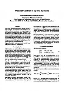
subject to (9) where we try to determine the optimal event times and physical states at these times. Once these are known, the relationship (15) is used to determine the optimal controls for the N time intervals involved in the operation of the system. The hybrid controller for coordinating the two problems above operates as follows (see Figure 1): 1. System identification: the physical dynamics, g, the costs associated with the physical dynamics, φ, the temporal dynamics, f , and the costs associated with the temporal dynamics, ψ, are all input to the controller. 2. Lower-level problem, parameterized by si : The lower level controller solves (14) to determine θi (zi0 , zif , si ) and u∗i (zi0 , zif , si ) for all i = 1, . . . , N . 3. Higher-level problem: The higher level controller solves (16) to determine the optimal values s∗i , (zi0 )∗ , and (zif )∗ for all i = 1, . . . , N . 4. Lower-level problem, given s∗i : The lower level controller evaluates u∗i = u∗i ((zi0 )∗ , (zif )∗ , s∗i ) for all i = 1, . . . , N .

The explicit solutions of the two problems depend on the nature of the respective cost functions and dynamics. In some cases, the higher-level problem is greatly simplified when the eventdriven dynamics involve a single exogenous event process, while in other cases the event-driven dynamics introduce nondifferentiabilities that prohibit the use of standard optimization methods. In the next two sections, we consider two different classes of hybrid systems with different characteristics, illustrating the major differences between the two problem levels (see also [13]).

7

xi = xi −1 + f i (•) α, ψ

s* Higher-level Controller s*

θ*

Lower-level Controller g, φ u*

z&i = gi ( zi , ui ) Figure 1: Hybrid Controller Operation

3

Switched Linear Systems

Let us consider a class of hybrid systems consisting of linear time-invariant time-driven dynamics and associated quadratic criteria for all modes. In order to illustrate the hierarchical decomposition approach and obtain some explicit numerical results, we limit ourselves to a specific two-mode example as follows: z˙1 = u1 ,

z1 (x0 ) = z0

z˙2 = αz2 + u2 ,

z2 (x1 ) = z1 (x1 )

The event-driven dynamics determining how to switch between modes have the simple form given in (3): x1 = x0 + s1 (z1 , u1 ) x2 = x1 + s2 (z2 , u2 ) The cost to minimize is J = φ1 (s1 ) + φ2 (s2 ) + ψ2 (x2 ) Note that the cost is separable so the decomposition approach previously described may be applied. We consider quadratic costs for the physical process, so that (12) in this case becomes °2 1 Z si 1 ° ° f d° φi (si ) = h °zi − zi ° + r kui (t)k2 + q kzi (t)k2 dt 2 2 0

where a quadratic cost is imposed on the deviation of the final state zif = zi (xi ) from some desired value zid . In particular, let Z s1 1 r1 u21 (t)dt φ1 (s1 ) = 2 0 Z s2 1 1 f f 2 φ2 (s2 ) = h(z2 − zd ) + r2 u22 (t)dt 2 2 0 8

We also consider a quadratic cost on the final time x2 : ψ2 (x2 ) = βx22 Let us now consider the lower-level problem which, for each mode, is a standard Linear Quadratic (LQ) problem [1]. The Hamiltonian for the first stage [x0 , x0 + s1 ) of the physical process is 1 H1 (t) = r1 u21 (t) + p1 (t)u1 (t) 2 where p1 (t) is the costate for the first stage, hence the optimality conditions for the first stage are z˙1 (t) = u1 (t) p˙1 (t) = 0 r1 u1 (t) + p1 (t) = 0 Therefore, the optimal control in the first stage is a constant u1 and we get z1 (x1 ) − z1 (x0 ) z1f − z10 u1 = ≡ s1 s1 and 1 θ1 (z10 , z1f , s1 ) = min φ1 (s1 ) = r1 u21 s1 u1 2 i2 1 r1 h f = z1 − z10 2 s1

Similarly, for the second stage the Hamiltonian is

1 H2 (t) = r2 u22 (t) + p2 (t)u2 (t) + αp2 (t)z2 (t) 2 where p2 (t) is the costate for the second stage, hence the optimality conditions for the second stage are z˙2 (t) = αz2 (t) + u2 (t) p˙2 (t) = −αp2 (t)

r2 u2 (t) + p2 (t) = 0 Therefore, u2 (t) = − and

³ ´ 2α z2f − z20 eαs2 (e−αs2 − eαs2 )

e−αt

θ2 (z20 , z2f , s2 ) = min φ2 (s2 ) u2

1 = h(z2f − zdf )2 + 2 9

³ ´2 r2 α z2f − z20 eαs2 (eαs2 − e−αs2 )

e−αs2

The higher-level optimization problem (16) becomes   ´2 ³ f 0 eαs2 ³ ´ ´ ³ z − z αr 2 2 2 2 2 1  1 r1 f  z1 − z10 + h z2f − zdf + + βx22  min  2αs 2 (e 2 − 1) s1 ,s2 ,z10 , 2 s1 z20 ,z1f ,z2f

subject to z10 = z0 , z20 = z1f , s1 , s2 ≥ 0, and x2 = s1 + s2 . The resulting reduced optimization problem is · ´2 1 ³ ´2 1 r1 ³ f f f z h z − z + − z (17) min 0 1 2 d s1 ,s2 , 2 s1 2 f f z1 ,z2

+ where s1 , s2 ≥ 0.

´2 ³ z2f − z1f eαs2 αr2 (e2αs2 − 1)

+ + β((s1 + s2 )2

i

The optimality conditions are given in terms of four algebraic equations which can be solved to yield s1 , s2 , z1f , and z2f , assuming s1 > 0 and s2 > 0 (if we allow s1 = 0 and s2 = 0, we get z1f = z0 and z2f = z1f , respectively): ´ ³ f f αs2 αr2 2 z − z e 2 1 r1 f (z1 − z0 ) = s1 (eαs2 − e−αs2 ) ³ ´ 2 z2f − z1f eαs2 αr2 h(z2f − zdf ) = − (e2αs2 − 1) r1 (z1f − z0 )2 = 4βs21 (s1 + s2 ) ³ ´ ³ ´2 α2 r2 z2f − z1f eαs2 (z1f eαs2 ) α2 r2 e2αs2 z2f − z1f eαs2 + β(s1 + s2 ) = (e2αs2 − 1) (e2αs2 − 1)2

For a numerical example, setting r1 = 2, r2 = 10, h = 10, zd = 10, z0 = 0, α = 1 and β = 10, yields the following solution: It is optimal to start operating in the first mode with constant control u1 (t) = 5.72 for t ∈ [0, x1 ) and switch to the second mode at time x1 = 0.4 when z1f = 2.29. The system operates in the second mode with control u2 (t) = 1.66e−t until time x2 = 1.64 when z2f = 9.67. In this type of a simple switched linear system, the main complexity lies in the fact that the LQ f problems involved are coupled through the continuity requirements zi0 = zi−1 associated with the ith mode switch. This leads to a higher-level nonlinear optimization problem such as (17). Obtaining an analytic form for this nonlinear optimization problem depends on the availability of a closed-form solution for the LQ problems associated with each mode at the lower level of the decomposition. Except for relatively simple cases such as the one considered above, this is not possible, and numerical techniques must be invoked. This has motivated recent work by Xu and Antsaklis [12] making use of the sensitivities of the optimal cost at the lower level with respect to the switching times x1 , . . . , xN involved. On the other hand, the presence of more challenging event-driven dynamics shifts the main complexity burden to the higher-level problem, as discussed in the next section. 10

4

Switched Systems with Nondifferentiable Event-Driven Dynamics

In the problem of the previous section, the switching time dynamics are determined through xi = xi−1 + si (zi , ui )

(18)

which is a simple linear relationship. Thus, as already mentioned, the complexity is concentrated in determining the optimal amount of time spent in mode i, si (zi , ui ), whereas the event driven dynamics yielding the switching time sequence {x1 , x2 , . . .} in this case are extremely simple. The situation is very different when switching times are dependent upon two or more event processes, in which case we must resort to (9) and analyze the timed automaton that coordinates these processes. In what follows, we shall discuss a class of systems where the event-driven switching time dynamics are described by xi = max(xi−1 , ai ) + si (ui )

(19)

where {ai }, i = 1, . . . , N , is a given sequence of event times corresponding to an asynchronous event process operating independently of the physical processes {zi (t), t ∈ [xi−1 , xi )}. In fact, the “max-plus” recursive equation (19) is the Lindley equation, well-known in queueing theory [2], describing the times at which “customers” depart from a simple queueing system; in this case, ai is the ith customer’s arrival time and si (ui ) is the time required to process the ith customer, dependent upon some control ui . In comparing (19) to (18), note that the key difference is the presence of the max function, which introduces a nondifferentiable component into the solution of the overall problem. Thus, the problem we consider here is (13), subject to (2) and (19) and u as defined in (11). This problem is largely motivated by the structure of many manufacturing systems: Discrete entities (referred to as jobs) move through a network of workcenters which process the jobs so as to change their physical characteristics according to certain specifications. Associated with each job is a temporal state and a physical state. The temporal state of a job evolves according to event-driven dynamics and includes information such as the waiting time or departure time of the job at the various workcenters. The physical state evolves according to time-driven dynamics which, depending on the particular problem being studied, describe changes in such quantities as the temperature, size, weight, chemical composition, or some other measure of the “quality” of the job. The interaction of time-driven with event-driven dynamics leads to a natural trade-off between temporal requirements on job completion times and physical requirements on the quality of the completed jobs. For example, while the physical state of a job can be made arbitrarily close to a desired “quality target”, this usually comes at the expense of long processing times resulting in excessive inventory costs or violation of constraints on job completion deadlines. Our objective, therefore, is to formulate and solve optimal control problems of the form (13) which capture such trade-offs. In the context of manufacturing systems, the mode switches correspond to jobs that we index by i = 1, . . . , N . We shall limit ourselves to a single-stage process modeled as a single-server queueing system. The objective is to process N total jobs. The server processes one job at a 11

time on a first-come first-served nonpreemptive basis (i.e., once a job begins service, the server cannot be interrupted, and will continue to work on it until the operation is completed). Jobs arriving when the server is busy wait in a queue whose capacity is ≥ N . As job i is being processed, its physical state zi , evolves according to time-driven dynamics of the general form (2), where xi−1 is the time when processing begins. The control variable ui will be assumed here to be scalar and not time-dependent for simplicity; it is used to attain a final desired physical state corresponding to a target “quality level”. Specifically, if the service time for the ith job is si (ui ) and Γi (ui ) is a given set (e.g., a threshold above which zi satisfies a desired quality level), then the control ui is chosen to satisfy the stopping rule si (ui )

(

"

= min t ≥ 0 : zi (xi−1 + t) =

Z

#

xi−1 +t

xi−1

)

(20)

gi (zi , ui , ν)dν + ζi ∈ Γi (ui )

where ui takes a fixed constant value during the interval [xi−1 , xi−1 + t), and the “min” is assumed to exist. On the other hand, the temporal state of the ith job, xi , represents the time when the job completes processing and departs from the system. Letting ai be the arrival time of the ith job, the event-driven dynamics describing the evolution of the temporal state are given by (19). A typical state trajectory if this type of system is shown in Fig. 2. Note that the interval (x1 , a2 ] in this example corresponds to an “idle period” for the workcenter and causes the second switching time to become, from (19), x2 = max(x1 , a2 ) + si (ui ) = a2 + si (ui ).

Physical State, z

. zi = gi(zi,ui,t)

.

. a1

…

x1

.

.

a2 a3 x2

ai xi

…

Temporal State, x xi+1 = max(xi-1,ai) + si(ui)

Figure 2: Typical state trajectory

To summarize, the optimization problem of interest here is min

u1 ,...,uN

N X

[φi (ui ) + ψi (xi )]

i=1

s.t. xi = max(xi−1 , ai ) + si (ui ) 12

(21)

where a1, . . . , aN is a given input sequence of event times and si (ui ) is specified through (20). This is similar in form to classical discrete-time optimal control problems commonly found in the literature (e.g., [1]) except for two issues. First, the index i = 1, . . . , N does not count time steps, but rather asynchronously departing jobs. Second, the presence of the “max” function in the state equation (19) prevents us from using standard gradient-based techniques, since it introduces a nondifferentiability at the point where ai = xi−1 . In effect, (21) formulates an optimal control problem for a DES with dynamics given by (19), where the control variables regulate interevent times. In order to overcome the nondifferentiability introduced through the max in (19), one can resort to nonsmooth optimization techniques, as in [14]. Under some reasonable assumptions on φi (ui ) and ψi (xi ), it is shown that a unique solution exists and can be obtained explicitly through an algorithm based on calculating generalized gradients and solving a Two Point Boundary Value Problem (TPBVP). However, it turns out that one can exploit the structure of state trajectories, as seen in Fig. 2, to decompose the overall problem (21) into a collection of simpler nonlinear constrained optimization problems. A key observation is that, unlike the problem considered in the previous section, there is no coupling of physical states when a mode switch occurs: after a job is processed and departs at time xi with physical state zi (xi ), the new mode corresponds to a completely new job with physical state zi+1 (x+ i ) which is independent of zi (xi ). Taking a closer look at the state trajectory in Fig. 2, observe that it consists of periods during which the workcenter is busy, separated by intervals during which it becomes temporarily idle, as in (x1 , a2 ). Recalling (19), note that all jobs processed within a busy period are such that xi−1 ≤ ai , therefore, by (19) they satisfy xi = xi−1 + si (ui ) where we allow for the possibility that a control ui is selected so that xi−1 = ai ; we refer to jobs with the property that they depart exactly when the next job arrives as “critical”, a manifestation of the intuitive fact that processing jobs on a “just in time” basis is occasionally (but not always) optimal. On the other hand, if a job initiates a busy period (equivalently, terminates an idle period), then xi = ai + si (ui ) To formalize this partition of the state trajectory into “busy” and “idle” periods, we make the following definitions : Definition 1. An idle period is a time interval (xk , ak+1 ) such that xk < ak+1 for any k = 1, ..., N − 1. Definition 2. A Busy Period (BP) is a set of contiguous jobs {k, ...., n}, 1 ≤ k ≤ n ≤ N such that the following conditions are satisfied 1. xk−1 < ak 2. xn < an+1 3. xi ≥ ai+1 for every i = k, ..., n − 1. 13

Definition 3. A busy-period structure is a partition of the jobs 1, ...., N into busy periods. Obtaining an explicit solution to problem (21) is tantamount to identifying the BP structure of the optimal state trajectory (sample path) and then solving a nonlinear optimization problem within each BP. If a BP is defined by the job indices (k, n), then we denote this problem by Q(k, n): Q(k, n) : min

u1 ,...,uN

N i X X {φi (ui ) + ψi (ak + sj (uj ))} : si (ui ) ≥ 0} i=k

s.t. ak +

j=k

i X j=k

(22)

sj (uj ) ≥ ai+1 ,

i = k, ...., n − 1

P Note that we have set ψi (xi ) = ψi (ak + ij=k sj (uj )) since, within a BP, xj = aj + sj (uj ) for all i = k, ...., n − 1. The constraint represents the requirement xi ≥ ai+1 for any job i = k, ...., n − 1 belonging to the BP. Let us also impose some basic conditions on the cost functions φi (ui ) and ψi (xi ): Assumption 1: For each i = 1, . . . , N , φi (·) is strictly convex, twice continuously differentiable, i and monotonically decreasing with limui →0+ φi (ui ) = − limui →0+ dφ dui = ∞ and limui →∞ φi (ui ) = i limui →∞ dφ dui = 0. Assumption 2: For each i = 1, . . . , N , ψi (·) is strictly convex, twice continuously differentiable, and its minimum is obtained at a finite point δi . In addition, let restrict ourselves to controls ui that affect the processing time of the ith job linearly: Assumption 3: For each i = 1, . . . , N , si (·) is monotonically increasing and linear. The latter assumption allows us, for simplicity, to replace si (ui ) by ui and directly control all processing times. Moreover, note that under the first two assumptions problem Q(k, n) is a convex constrained optimization problem which is readily solved using standard techniques. We denote the (unique) solution to this problem by u∗i (k, n), i = k, ...., n and the corresponding event times by x∗i (k, n), i = k, .... Under these conditions, the following result provides a crucial necessary and sufficient condition for identifying a BP on the optimal state trajectory making use of solutions. Theorem 4.1 (Cho et al. [15]) Jobs k, . . . , n constitute a single busy period on the optimal sample path if and only if the following conditions are satisfied: 1. ak > x∗k−1 2. x∗i (k, i) ≥ ai+1 for all i = k, . . . , n − 1 3. x∗n (k, n) < an+1 14

The significance of this necessary and sufficient condition is best understood as follows. Given N jobs, the total number of possible BPs is given 2N−1 . Thus, the complexity of exploring all BP structutres in order to determine the optimal one is combinatorial in nature. However, this complexity is reduced to linear using the theorem above: One proceeds forward in time sequentially solving a problem of the form Q(k, n), with k = 1 initially, until the condition x∗n (k, n) < an+1 is satisfied for some n ≥ k, at which point a BP defined by (k, n) is identified. The process then repeats for a new problem Q(n + 1, m) with m = n + 1, n + 2, . . . until a new BP is similarly identified. This gives rise to the Forward Algorithm (FA) presented in [15]. It is easy to see that the complexity of the FA is of the order of N convex constrained optimization problems of the form (22). In fact, one can improve the efficiency of the FA even further, as described in [16].

5

Conclusions

As time-driven and event-driven systems are rapidly merging, giving rise to a class of “hybrid” dynamic systems, the field of optimal control is presented with an opportunity to expand its horizons, combining the fundamental principles on which it was originally conceived with new ideas that must tackle new forms of complexities. Some of these complexities are purely combinatorial in nature, the result of discrete elements in the problem such as switching events and modes to choose form, which enlarge an already large state space. Others are the result of nonlinear dynamics, including the type of nondifferential behavior one encounters in DES. Yet another form of complexity, which was only briefly mentioned in Section 1, is due to the stochastic nature of many state and/or input variables of interest. In order to deal with these unavoidable and sometimes new types of complexities, it is clear that we have to go beyond existing methods and to try and exploit any features present in the structure of a system or the optimization problem itself. In this paper, we aimed to show how a natural hierarchical decomposition of at least some classes of hybrid systems can simplify the task of solving optimal control problems. Still, in most cases, one must resort to numerical techniques in order to obtain explicit solutions, and this is before even considering the issue of selecting over a set of feasible modes when a switch occurs or seeking solutions that are in some sort of feedback form useful in practice. In the case of the optimal control problem (21), we have been able to take advantage of a different type of decomposition (over time, as opposed to over the system structure). However, we limited ourselves to a scalar problem and it is unclear whether a similar efficient decomposition can be used in a vector setting (e.g., a manufacturing system consisting of multiple workcenters). Finally, an interesting issue that this new line of research has brought up is that of applying Perturbation Analysis (PA) methods to hybrid systems in a way similar to the successful development of PA for DES (see [2],[17]) that has contributed to the solution of some complex optimization problems. Looking at problems in the fields of manufacturing, communication networks, transportation, and command-control systems, one is struck by the natural way in which hybrid systems manifest themselves and optimization problems arise which the PA framework

15

can help solve through on-line techniques that exploit the structure of sample paths and the data one can readily extract from them. There are promising signs in this direction (e.g., see [18]), a fact that should be gratifying to Larry Ho, since Perturbation Analysis for DES is also an area that he pioneered in the early 1980s.

References [1] A. E. Bryson and Y. C. Ho, Applied Optimal Control. Hemisphere Publishing Co., 1975. [2] C. G. Cassandras and S. Lafortune, Introduction to Discrete Event Systems. Kluwer Academic Publishers, 1999. [3] P. J. Antsaklis, ed., Proceedings of the IEEE, vol. 88, 2000. [4] M. S. Branicky, V. S. Borkar, and S. K. Mitter, “A unified framework for hybrid control: Model and optimal control theory,” IEEE Trans. on Automatic Control, vol. 43, no. 1, pp. 31—45, 1998. [5] B. Piccoli, “Hybrid systems and optimal control,” in Proceedings of 37th IEEE Conf. On Decision and Control, pp. 13—18, Dec. 1998. [6] H. J. Sussmann, “A maximum principle for hybrid optimal control problems,” in Proceedings of 38th IEEE Conf. On Decision and Control, pp. 425—430, Dec. 1999. [7] S. Hedlund and A. Rantzer, “Optimal control of hybrid systems,” Proceedings of 38th IEEE Conf. On Decision and Control, pp. 3972—3977, 1999. [8] X. Xu and P. J. Antsaklis, “A dynamic programming approach for optimal control of switched systems,” in Proceedings of 39th IEEE Conf. On Decision and Control, pp. 1822— 1827, Dec. 2000. [9] A. Bemporad, F. Borelli, and M. Morari, “Optimal controllers for hybrid systems: Stability and piecewise linear explicit form,” in Proceedings of 39th IEEE Conf. On Decision and Control, pp. 1810—1815, Dec. 2000. [10] A. Giua, C. Seatzu, and C. V. D. Mee, “Optimal control of switched autonomous linear systems,” in Proceedings of 40th IEEE Conf. On Decision and Control, pp. 2472—2477, Dec. 2001. [11] K. Gokbayrak and C. G. Cassandras, “Hybrid controllers for hierarchically decomposed systems,” in Proceedings of 3rd Intl. Workshop on Hybrid Systems: Computation and Control, pp. 117—129, March 2000. [12] X. Xu and P. J. Antsaklis, “Optimal control of switched systems: New results and open problems,” Proceedings of the ACC, pp. 2683—2687, 2000. [13] K. Gokbayrak and C. G. Cassandras, “A hierarchical decomposition method for optimal control of hybrid systems,” in Proceedings of 39th IEEE Conf. On Decision and Control, pp. 1816—1821, December 2000. 16

[14] C. G. Cassandras, D. L. Pepyne, and Y. Wardi, “Optimal control of a class of hybrid systems,” IEEE Trans. on Automatic Control, vol. AC-46, no. 3, pp. 398—415, 2001. [15] Y. C. Cho, C. G. Cassandras, and D. L. Pepyne, “Forward decomposition algorithms for optimal control of a class of hybrid systems,” Intl. Journal of Robust and Nonlinear Control, vol. 11, no. 5, pp. 497—513, 2001. [16] P. Zhang and C. G. Cassandras, “An improved forward algorithm for optimal control of a class of hybrid systems,” in Proceedings of 40th IEEE Conf. On Decision and Control, pp. 1235—1236, Dec. 2001. [17] Y. C. Ho and X. Cao, Perturbation Analysis of Discrete Event Dynamic Systems. Dordrecht, Holland: Kluwer Academic Publishers, 1991. [18] C. G. Cassandras, Y. Wardi, B. Melamed, G. Sun, and C. G. Panayiotou, “Perturbation analysis for on-line control and optimization of stochastic fluid models,” IEEE Transactions on Automatic Control, 2002. To appear.

17