OPTIMAL CONTROL OF DISSIPATIVE TWO-LEVEL

OPTIMAL CONTROL OF DISSIPATIVE TWO-LEVEL QUANTUM SYSTEMS BERNARD BONNARD∗ AND DOMINIQUE SUGNY† Abstract. The objective of this article is to apply recent developments in geometric optimal control to analyze the time minimum control problem of dissipative two-level quantum systems whose dynamics is governed by the Lindblad equation. We focus our analysis on the case where the extremal Hamiltonian is integrable. Key words. Optimal control, conjugate and cut loci, quantum control AMS subject classifications. 49K15, 70Q05

1. Introduction. We consider a dissipative two-level quantum system whose dynamics is governed by the Lindblad equation which takes the following form in suitable coordinates q = (x, y, z), i.e., in the coherence vector formulation of density matrix [1, 14]: x˙ = −Γx + u2 z y˙ = −Γy − u1 z z˙ = γ− − γ+ z + u1 y − u2 x.

(1.1)

We refer to [8] and [15] for the details of the model. We recall that x and y are related to off-diagonal terms of the density matrix of the system and z to the difference of population between the two states. In (1.1), Λ = (Γ, γ− , γ+ ) is a set of parameters such that Γ ≥ γ+ /2 > 0 and γ+ ≥ |γ− | which describes the interaction of the two-level system with the environment. More precisely, Γ is the dephasing rate and γ+ and γ− are respectively equal to γ12 + γ21 and γ12 − γ21 where the coefficients γ12 and γ21 are the population relaxation rates. The control is the complex Rabi frequency u = u1 + iu2 of the laser field which is assumed to be in resonance with the frequency of the two-level system [9]. The physical state belongs to the Bloch ball, |q| ≤ 1, which is invariant for the dynamics considered. The system can be written shortly as a bilinear system q˙ = F0 (q) + u1 F1 (q) + u2 F2 (q)

(1.2)

and in order to minimize the effect of dissipation, we consider the time minimum control problem for which, up to a rescaling on the set of parameters Λ, the control RT bound is |u| ≤ 1. The energy minimization problem with the cost 0 |u|2 dt where the time T is fixed but the control bound is relaxed can also be considered and shares similar properties. A first step in the analysis of such systems is contained in [15]. Assuming u real, the problem can be reduced to the time-optimal control of a two-dimensional system y˙ = −Γy − u1 z z˙ = γ− − γ+ z + u1 y,

(1.3)

∗ Institut de Math´ ematiques de Bourgogne, UMR CNRS 5584, 9 Avenue Alain Savary, BP 47 870 F-21078 DIJON Cedex FRANCE ([email protected]). † Institut Carnot, UMR CNRS 5209 9 Avenue Alain Savary, BP 47 870 F-21078 DIJON Cedex FRANCE ([email protected]).

1

2 with the constraint |u1 | ≤ 1. For such a problem, the geometric optimal control techniques for single-input two-dimensional systems presented in [11] succeed to make the time-optimal synthesis for every values of parameters (Γ, γ− , γ+ ). In order to complete the analysis in the bi-input case, a different methodology has to be applied and we shall make an intensive use of techniques and results develop in a parallel research project to minimize the transfer of a satellite between two elliptic orbits (see [8]). Such techniques are twofold. First of all, the maximum principle will select extremal trajectories, candidates as minimizers and solutions of an Hamiltonian equation. A geometric analysis will identify the symmetry group of the system and find suitable coordinates to represent the Hamiltonian. A consequence of this analysis is the fact that, in the case γ− = 0, the extremal system is integrable and if Γ = γ+ , the problem can be in addition reduced to a 2D-almost Riemannian problem on a two-sphere of revolution for which a complete analysis comes from [5]. We take advantage of this property to analyze the general integrable case γ− = 0 using continuation methods on the set of parameters, while the analysis fits in the geometrical framework of Zermelo navigation problems [3]. Secondly, having selected extremal trajectories, second-order conditions using the variational equation and implemented in the COTCOT code [6] allow to determine first conjugate points forming the conjugate locus which are points where locally extremals cease to be optimal. Combined with the geometric analysis, we can construct the cut locus which is formed by points where extremals cease to be globally optimal. The organization of this article is the following. In section 2, we recall the maximum principle and the concept of conjugate points associated to second-order optimality conditions. In section 3, we present the geometric analysis of the system, followed in section 4 by a thorough analysis of the so-called Grusin problem on a twosphere of revolution. This problem is generalized into a Zermelo navigation problem suitable to our analysis. In section 5, we study the properties of the extremals to analyze the optimal trajectories, combining analytic and numerical methods. 2. Geometric optimal control. 2.1. Maximum principle. We consider the time minimum problem with fixed extremities q0 and q1 . For a smooth system written q˙ = F (q, u), with q ∈ Rn and a control domain U which is a compact subset of Rn , we have: Proposition 2.1. If (u, q) is an optimal control trajectory pair on [0, T ] then there exists an absolutely continuous non-zero vector function (p, p0 ) ∈ Rn × R such that almost everywhere on [0, T ], we have: q˙ =

∂H ∂H (q, p, u), p˙ = − (q, p, u) ∂p ∂q

(2.1)

and H(q, p, u) = M (q, p)

(2.2)

where H(q, p, u) = hp, F (q, u)i + p0 , p0 being a non positive constant; M is defined by M (q, p) = M axu∈U H(q, p, u) and M is zero everywhere. Definition 2.2. The mapping H is called the pseudo-Hamiltonian. A triple (q, p, u) solution of (2.1) and (2.2) is called extremal while the component q is called an extremal trajectory and p is an adjoint vector. Application: We consider the time-minimum control problem for a system of the

3 Pm form q˙ = F0 (q) + i=1 ui Fi (q) with m ≥ 2, u = (u1 , · · · , um ), |u| ≤ 1. We introduce the Hamiltonian lifts Hi = hp, Fi (q)i, i = 0, 1, · · · , m of the vector fields Fi and the set Σ such that Hi = 0 for i = 1, · · · , m. Then the maximization condition (2.2) leads to the following result. pPm 2 Proposition 2.3. Outside Σ, an extremal control is given by ui = Hi / i=1 Hi , i = 1 · · · , m and extremal pairs z = (x, p) are solutions of the smooth true Hamil~ r (z) with Hr (z) = H0 (z) + (Pm H 2 )1/2 . tonian vector field H i=1 i Definition 2.4. The surface Σ is called the switching surface and the solutions ~ r (z) are called extremals of order zero. To be optimal, they have to satisfy of H Hr (z) ≥ 0 and those with Hr (z) = 0 are called abnormal. An important but straightforward result is the following proposition. Proposition 2.5. Extremal trajectories of order zero correspond to singularities of the end-point mapping E q0 ,T : u ∈ L∞ [0, T ] 7→ q(T, q0 , u)

(2.3)

where q(·, q0 , u) denotes the response to u with initial condition q0 and such that the control is restricted to the (m − 1)-sphere |u| = 1. 2.2. Second-order optimality conditions. From the previous result, we can apply the concepts and algorithms presented in [6] to compute second-order optimality conditions in the smooth case, when the control domain U is a manifold, u being restricted to the unit sphere. The framework of this computation is next recalled. The concept of conjugate point: Since U is a manifold, we may assume locally that U = Rm−1 and the maximization condition (2.2) leads to ∂H ∂2H = 0, ≤ 0. ∂u ∂u2

(2.4)

Our first assumption is the strong Legendre-Clebsch condition: (H1) The Hessian ∂ 2 H/∂u2 is negative definite along the reference extremal. From the implicit function theorem, an extremal control can be locally defined as a smooth function of z = (x, p) and plugging u into H defines a smooth true Hamiltonian Hr . Setting M = Rn and using Hamiltonian formalism, we introduce: Definition 2.6. Let z = (x, p) be a reference extremal defined on [0, T ]. The variational equation ~ r (z(t))δz δ z˙ = dH

(2.5)

is called the Jacobi equation. A Jacobi field is a non trivial solution δz = (δx, δp). It is said vertical at time t if δx(t) = 0. The following standard result is crucial. ~ r (L0 )] be its Proposition 2.7. Let L0 be the fiber Tq∗0 M and let Lt = exp[tH ~ r . Then Lt is a Lagrangian image by the one parameter subgroup generated by H manifold whose tangent space at z(t) is spanned by Jacobi fields vertical at t = 0. Moreover, the rank of the restriction to Lt of the projection Π : (q, p) 7→ q is at most (n − 1). We next formulate the relevant generic assumptions using the end-point mapping. Assumptions:

4 1. (H2) On each subinterval [t0 , t1 ], 0 < t0 < t1 ≤ T , the singularity of E q(t0 ),t1 −t0 is of codimension one for u|[t0 ,t1 ] . 2. (H3) We are in the normal case Hr 6= 0. As a result, on each subinterval [t0 , t1 ] there exists up to a positive scalar an unique adjoint vector p such that (q, p, u) is extremal. Definition 2.8. We fix q0 = q(0) and we define the exponential mapping: ~ r (q(0), p(0))]) expq0 : (p(0), t) 7→ Π(exp[tH where p(0) is a (n − 1) dimensional vector, normalized with Hr = 1. Definition 2.9. Let z = (x, p) be the reference extremal on [0, T ]. Under our assumptions, a time 0 < tc ≤ T is called conjugate if the mapping expq0 is not an immersion at (p(0), tc ) and the point q(tc ) is said to be conjugate to q0 . We denote t1c the first conjugate time and C(q0 ) the conjugate locus formed by the set of first conjugate points taking all extremal curves. We get: Theorem 2.10. Let z(t) = (q(t), p(t)) be a reference extremal on [0, T ] satisfying assumptions (H1), (H2) and (H3). Then it is optimal in the L∞ -norm topology on the set of controls up to the first conjugate time t1c . Moreover, if t 7→ q(t) is one-to-one then it can be embedded into a set W , image by the exponential mapping expq(0) of N × [0, T ], where N is a conical neighborhood of p(0). For T < t1c , the reference extremal trajectory is time minimal with respect to all trajectories contained in W . In order to get global optimality results, it is necessary to glue together such microlocal sets. We use for that the following concepts. Definition 2.11. Given an extremal trajectory, the first point where it ceases to be optimal is called the cut point and taking all the extremals starting from q0 , they will form the cut locus Cut(q0 ). The separating line L(q0 ) is formed by the set of points where two minimizers initiating from q0 intersect. 3. Geometric analysis of Lindblad equation. 3.1. Symmetry of revolution. If we apply to system (1.1) a change of coordinates defined by a rotation of angle θ around the z−axis: X = x cos θ + y sin θ Y = −x sin θ + y cos θ Z = z, and a similar feedback transformation on the control: v1 = u1 cos θ + u2 sin θ, v2 = −u1 sin θ + u2 cos θ, we obtain the system X˙ = −ΓX + v2 Z Y˙ = −ΓY − v1 Z Z˙ = γ− − γ+ Z + v1 Y − v2 X.

(3.1)

Hence, this defines a one dimensional symmetry group and by construction |u| = |v|. Therefore, we deduce that the time-minimum control problem (or the energy minimization problem) are invariant for such an action. Using cylindric coordinates x = r cos θ, y = r sin θ, z = z

5 and the dual variables p = (pr , pθ , pz ), the Hamiltonian Hr takes the form Hr = H0 + (H12 + H22 )1/2 = (−Γrpr + (γ− − γ+ )pz ) + (z 2 p2r +

z2 2 p + r2 p2z − 4zrpr pz )1/2 . r2 θ

In particular, the Bloch ball is foliated by meridian planes θ = constant in which the time-minimum synthesis is the one associated to system (1.3), where the control is scalar and described in [15]. More precisely, we have: Proposition 3.1. For the time-minimum control, θ is a cyclic coordinate and pθ is a first integral of the motion. The sign of θ˙ is given by pθ and if pθ = 0 then θ is constant and the extremal synthesis for an initial point on the z-axis is up to a rotation given by the synthesis in the plane θ = 0. Up to a rotation, the control u can also be restricted to the single-input control (u1 , 0). 3.2. Spherical coordinates. More properties can be seen using spherical coordinates: x = ρ sin φ cos θ, y = ρ sin φ sin θ, z = ρ cos φ and a similar feedback transformation. We obtain the system: ρ˙ = γ− cos φ − ρ(γ+ cos2 φ + Γ sin2 φ) γ− sin φ sin(2φ) φ˙ = − + (γ+ − Γ) + v2 ρ 2 θ˙ = −(cot φ)v1 .

(3.2)

and the corresponding Hamiltonian Hr = [γ− cos φ − ρ(γ+ cos2 φ + Γ sin2 φ)]pρ q γ− sin φ sin(2φ) +[− + (γ+ − Γ)]pφ + p2φ + p2θ cot2 φ. ρ 2 In this representation, (φ, θ) are the spherical coordinates on the unit sphere of revolution around the z-axis: θ is the angle of revolution and φ ∈]0, π[ is the angle of the meridian, φ = 0, π correspond respectively to the north and south poles. 3.3. Lie brackets computations. In order to complete the analysis, we immediately compute the Lie brackets up to length 3 for the system written in Cartesian coordinates as: q˙ = (G0 q + v0 ) + u1 G1 q + u2 G2 q where the Gi ’s are the matrices    −Γ 0 0 0 0  , G1 =  0 G0 =  0 −Γ 0 0 −γ+ 0

0 0 1

   0 0 0 1 −1  , G2 =  0 0 0  0 −1 0 0

and t v0 is the vector (0, 0, γ− ). It can be lifted into a right-invariant control system on the semi-direct product GL(3, R) ×S R3 identified to the subgroup of matrices of GL(4, R) of the form: µ ¶ 1 0 , v ∈ R3 , g ∈ GL(3, R) v g

6 which acts on R4 identified to the set of vectors µ ¶ 1 , q ∈ R3 . q To construct affine vector fields, we use the induced action of the Lie algebra (a, A)·q = Aq + a and Lie brackets are given by [(a, A), (b, B)] = [Ab − Ba, AB − BA]. The control distribution is D = Span{G1 , G2 } and we have:   0 −1 0 [G1 , G2 ] = G3 =  1 0 0  . 0 0 0 In particular, we obtain that {G1 , G2 }A.L. = so(3) and hence that the system on SO(3): dX = (u1 G1 + u2 G2 )X dt is controllable. For the linear action, it defines a controllable system on the unit sphere. This action has however singularities: • at 0, the orbit is 0. • The set on R2 where G1 and G2 are collinear is the whole plane z = 0 and restricted to the unit sphere of revolution, it corresponds to the equator. To analyze the effect of the drift term associated to dissipation, we use     0 0 0 0 0 1 [G0 , G1 ] = (Γ − γ+ )  0 0 1  , [G0 , G2 ] = (γ+ − Γ)  0 0 0  0 1 0 1 0 0 and [G0 , G3 ] = 0. Moreover, we have    0 0 0 1 0 [G1 , [G0 , G1 ]] = 2(Γ−γ+ )  0 1 0  , [G2 , [G0 , G2 ]] = 2(γ+ −Γ)  0 0 0 0 −1 0 0

 0 0 . −1

Those computations reveal the singularity at γ+ = Γ, γ− = 0 that we describe in the next proposition. Proposition 3.2. In the case γ− = 0, γ+ = Γ, the radial component ρ is not controllable and the time-minimum control problem is an almost Riemannian problem on the two-sphere of revolution for the metric in spherical coordinates g = dφ2 + tan2 φdθ2 with Hamiltonian H = 21 (p2φ + p2θ cot2 φ). Definition 3.3. The almost Riemannian metric g = dφ2 + tan2 φdθ2 is called the Grusin model on the two-sphere of revolution. Such a metric appears in quantum control in [10] and a similar metric in orbital transfer [4]. It will be analyzed in details in section 4 since it is the starting point of the analysis in the general case using a continuation method on the set of parameters. Another consequence of the previous computations is the controllability properties of the system and the structure of extremal trajectories.

7 3.4. Controllability properties. We recall that the Bloch ball |q| ≤ 1 is invariant. Indeed, introducing ρ2 = |q|2 , we get: ρρ˙ = −Γ(x2 + y 2 ) − γ+ z 2 + γ− z ≤ 0

(3.3)

which is strictly negative on the unit sphere except if x2 + y 2 = 0, |z| = 1 and γ+ = |γ− |. Using the representation (3.1) of the system in spherical coordinates, it is clear that we can control the angular variables φ and θ if the controls are not uniformly bounded. If |u| ≤ 1 then we have restrictions depending upon the set of parameters. For γ− = 0, the system is homogeneous and q = 0 is a fixed point. The accessibility set in fixed time is with non empty interior for a non-zero initial point, except in the case γ+ = Γ which corresponds to the Grusin model and for which the time and energy minimization problem are equivalent. The controllability properties for |u| ≤ 1 are clear in this case. Indeed, if |γ+ −Γ| < 2 then we can compensate the drift by feedback for the system on the two-sphere of revolution, while it is not the case for |γ+ − Γ| > 2. Proposition 3.4. Let q0 and q1 be two points in the Bloch ball |q| ≤ 1 such that q1 is accessible to q0 . Then there exists a time-minimum trajectory joining q0 to q1 . Moreover, every optimal trajectory is 1. either an extremal trajectory with pθ = 0, contained in a meridian plane, time-optimal solution of the two-dimensional system (1.3) where u = (u1 , 0). 2. either connection of smooth extremal arcs of order 0, solutions of the Hamil~ r with pθ 6= 0, while the only possible connections are tonian vector field H located in the equatorial plane φ = π/2. Proof. The control domain is convex and the Bloch ball is compact. Hence, we can apply the Filippov existence theorem [13]. In order to get a regularity result about optimal trajectories, much more work has to be done. This is due to the existence of a switching surface Σ : H1 = H2 = 0 in which we can connect two extremals arcs of order 0, provided we respect the Erdmann-Weierstrass conditions at the junction, i.e., the adjoint vector remains continuous and the Hamiltonian is constant. The set Σ can also contain singular arcs for which H1 = H2 = 0 holds identically. Hence, we can have intricate behaviors for such systems. In our case, the situation is simplified by the symmetry of revolution. Indeed, if pθ = 0 then the singularities are related to the classification of extremals in the single-input case, which is described in [15]. We cannot connect an extremal with pθ 6= 0 where pθ is the global first integral xpy − ypx to an extremal where pθ = 0 since the adjoint vector has to be continuous. Hence, the only remaining possibility is to connect two extremals of order 0 with pθ 6= 0 at a point of Σ leading to the conditions pφ = 0 and pθ cot φ = 0 in spherical coordinates. Since pθ 6= 0, one gets φ = π/2. The result is proved. 4. The Grusin model on a two-sphere of revolution with generalizations to Zermelo navigation problem. The Grusin model g = dφ2 + tan2 φdθ2 is a special case of metrics of the form dφ2 + G(φ)dθ2 on a two-sphere of revolution such that: • (H1) G0 (φ) 6= 0 on ]0, π/2[. • (H2) G(π − φ) = G(φ) (reflective symmetry with respect to the equator). They appear in optimal control in the orbit transfer, smooth at the equator or with a polar singularity, in quantum control and in various geometric problems, e.g., Riemannian problems on an ellipsoid of revolution. The importance of this control prob-

8 lem has justified the recent analysis of [5] that we complete next, using Hamiltonian formalism in order to make generalizations. We first interpret the Grusin model as a deformation of the round sphere. Definition 4.1. The standard homotopy between the Grusin model on the twoX sphere of revolution is gλ = dφ2 + Gλ (X)dθ2 where Gλ (X) = 1−λX , X = sin2 φ and λ ∈ [0, 1]. By construction, the metric is analytic for λ ∈]0, 1[ and for λ = 1, we have the Grusin model with a pole of order 1 at the equator. The first objective of this section is to show stability results concerning such metrics. We begin by the following general result. Proposition 4.2. Let dφ2 + G(φ)dθ2 be a smooth metric on a two-surface of revolution. Then, p2θ 1. Extremals are solutions of the Hamiltonian H = 12 (p2φ + G(φ) ) and arc-length parametrization amounts to restrict to H = 1/2. √ 2. If ψ is the angle of an unit-speed extremal with a parallel then pθ = G cos ψ is a constant and the extremal flow is Liouville integrable with two commuting first integrals H and pθ . √ 2 3. The Gauss curvature is K = − √1G ∂∂φ2G . We next make a complete analysis of the family of metrics gλ . 4.1. Curvature analysis. We have the following proposition. Proposition 4.3. For the family of metrics gλ , we have: cos2 φ . 1. The Gauss curvature is Kλ = (1−λ)−2λ (1−λ sin2 φ)3 λ sin(2φ) 2. K 0 (φ) = (1−λ [5(1 − λ) − 4λ cos2 φ]. sin2 φ)4 Hence K(φ) is non-constant and monotone non decreasing from the north pole to the equator for λ ∈]0, 1/5], while for λ ∈]1/5, 1[ it admits a minimum. For λ ∈]0, 1[, the curvature is maximum on the equator. The limit case λ = 1 corresponds to the Grusin case, for which the curvature is negative everywhere and tends to −∞ when φ tens to π/2.

4.2. Geometric properties. We next present the main properties of the extremal flow for a metric on a two-sphere of revolution g = dφ2 + G(φ)dθ2 satisfying (H1) and (H2) where g is smooth, except may be at the equator where it can admit a pole of order one. p2θ For such a family, we consider the smooth Hamiltonian H = 12 (p2φ + G(φ) ) and we restrict extremal curves to the level set H = 1/2. Fixing pθ , the parameterized family of corresponding Hamiltonians described the evolution of the (pφ , φ) variables p2

θ as solutions of a mechanical system for which V (φ) = G(φ) plays the role of amended potential. For pθ = 0, we get the meridian solutions. Hence, we can assume pθ 6= 0. Using assumption (H1), the only equilibrium point is for φ = π/2 and pφ = 0. The normalization H = 1/2 gives p2θ = G(φ) which is finite in the non-singular case. This leads to the equator solution only in the regular case. For the remaining trajectories, the level set H = 1/2 is sufficient to analyze the behaviors of φ. Indeed, it is a compact set, symmetric for the two reflections with respect to the φ-axis and the equator φ = π/2 and defined respectively by the two transformations: pφ 7→ −pφ and φ 7→ π − φ. Every trajectory is periodic and ψ = π/2 − φ oscillates periodically between ψmax and −ψmax . There is also a relation between the period of oscillation T and the amplitude ψmax , depending upon pθ .

9 By symmetry, every trajectory is defined by its restriction to a quarter of period, that is the sub-arc starting from the equator ψ = 0 and reaching ψmax . The trajectory starting from (φ(0), pφ (0)) and reaching π − φ(0) after passing ψmax is chased by the trajectory starting from (φ(0), −pφ (0)) and reaching π − φ(0). They are distinct if pφ (0) 6= 0. Moreover, using the assumption (H2), we deduce easily that for fixed pθ , the extremals starting from (φ(0), θ(0)) with respectively pφ (0) and −pφ (0) intersect with equal length on the antipodal parallel. They are distinct if pφ (0) 6= 0. The case pφ (0) = 0 corresponds for an initial condition not on the equator to tangential arrival and departure at parallels φ(0) and π − φ(0); pφ (0) = 0 gives the equator solution in the non singular case. The only difference in the singular case is that the equator is not solution, and for trajectories departing from the equator the extremals are always tangential to the meridian, while the first return to the equator can be arbitrarily closed from the initial point. Finally, another obvious symmetry is a reflectional symmetry with respect to the meridian obtained by changing pθ into −pθ . As a consequence of this analysis, we deduce: Proposition 4.4. Let g = dφ2 + G(φ)dθ2 be a metric on a two-sphere of revolution, satisfying (H1) and (H2) and smooth except may be at the equator where it can admit a pole of order one. 1. Then except the meridian and the equator solution in the regular case, every extremal is such that ψ = π/2 − φ oscillates periodically between two symmetric parallels. The first return mapping to the equator p R : pθ ∈]0, G(π/2)[7→ ∆θ(pθ ), where ∆θ is the corresponding θ − variation of the extremal is well defined. 2. Assume pθ 6= 0 and pφ (0) 6= 0 then a) Fixing pθ , changing pφ (0) into −pφ (0) gives two distinct extremals with equal length intersecting on the antipodal parallel. b) Fixing pφ (0) and changing pθ into −pθ gives two distinct extremals with equal length intersecting on the opposite meridian. 4.3. Integrability. For the family of metrics gλ which fit in the previous geometric framework, we can be more precise and make a complete analysis. The Hamiltonians are: Hλ =

1 2 p2θ sin2 φ (pφ + ), Gλ (φ) = 2 Gλ (φ) 1 − λ sin2 φ

and using φ˙ = pφ , we get: Hλ =

1 ˙ 2 p2θ (1 − λ sin2 φ) [φ + ] 2 sin2 φ

which can be written Hλ =

1 ˙2 [φ + p2θ (cot2 φ + 1 − λ)]. 2

Therefore, Hλ = H1 + 12 p2θ (1 − λ) and parameterized by arc-length: Hλ = 1/2, one gets the level set H1 = 12 − 21 p2θ (1 − λ).

10 Hence the integration of the Grusin case gives the general solution, and from the homotopy, the corresponding extremals fit not only in the same geometric framework, but also have the same transcendence. Lemma 4.5. The family of metrics gλ admits two commuting integrals independent of λ, pθ and H1 = 12 [p2φ + p2θ cot2 φ]. We next outline the integration method in the Grusin case to provide the computation of the first return mapping to the equator R obtained in [5]. We have H1 = 12 (φ˙ 2 + ν cot2 φ), ν > 0 and fixing the level set to 1/2, we get: (

dφ 2 1 − (ν + 1) cos2 φ . ) = dt sin2 φ

Taking the positive branch, we must evaluate the following expression Z sin φdφ =t (1 − (ν + 1) cos2 φ)1/2 to integrate. We use the relation Z cos φdφ 1 p = arcsin(m sin φ), 2 2 m 1 − m sin φ to deduce the form of the component φ of the general solution φ(t) = arcsin[

1 (sin(mt + K))] + π/2. m

To complete the integration, we write: θ˙ =

pθ − λpθ sin2 φ

and we use the formula: Z

√ dx 1 =√ arctan[ 1 − a tan x] 2 1−a 1 − a sin x

1 for a < 1 with the relation cos φ = − m sin(mt + K). A straightforward computation then leads to θ(t). Proposition 4.6. For the family of metrics gλ , we have:

R(pθ ) = π − √

απp λ p θ , α= . 2 1 − λ α + 1 α + 1 + αpθ

p In particular, if α > 0 then R0 (pθ ) < 0 < R00 (pθ ) on ]0, G(π/2)[. This property allows to evaluate conjugate and cut loci for the family of metrics that we next describe [5]. 4.4. Conjugate and cut loci. We can establish the following theorem about conjugate and cut loci. Theorem 4.7. • For λ = 0 (round sphere), the conjugate and cut loci of any point are reduced to the antipodal point.

11 • For 0 < λ < 1, the conjugate locus of a point different from a pole is diffeomorphic to a standard astroid, while the cut locus is a single branch of the antipodal parallel. Both are symmetric with respect to the opposite meridian. • For λ = 1 (Grusin case), the conjugate and cut loci of a point different from a pole and not on the equator are as above. For a point on the equator, the cut locus is the equator minus this point and for the conjugate locus, the cusps on the equator are transformed into folds at this point minus this point. Geometric interpretation: For the class of metrics gλ , the situation is clear. For the round sphere, all extremals starting from the equator intersect at the same antipodal point and the first return mapping is constant. For 0 < λ ≤ 1, the first return mapping is monotone, and in the singular case R(pθ ) → 0 as pθ → +∞. Since the cut locus of a point of the equator is formed by intersections with the equator of symmetric extremals, in the homotopy, the cut locus is pinched into a point for λ = 0, while it is stretched into the whole equator in the case λ = 1. 4.5. Zermelo navigation problem on the two-sphere of revolution. We introduce the following definition for the Zermelo problem. Definition 4.8. A Zermelo navigation problem on the two-sphere of revolution is a time-minimum problem of the form: 2 X dq = F0 (q) + ui Fi (q), |u| ≤ 1, dt i=1 ∂ ∂ + F02 (φ) ∂θ while F1 where the drift representing the current is of the form F01 (φ) ∂φ and F2 form outside the equator an orthonormal frame for a metric of the form g = dφ2 + G(φ)dθ2 . It is called reflectionaly symmetric with respect to the equator if • (H1) G0 (φ) 6= 0 on ]0, π/2[ • (H2) G(π − φ) = G(φ) • (H3) F01 (π − φ) = −F01 (φ), F02 = 0. If defines a Finsler geometric problem if |F0 | < 1 for the metric g. According to this classification, we have: Proposition 4.9. Assume γ− = 0 and consider the system (3.1) restricted to the two-sphere:

sin(2φ)(γ+ − Γ) φ˙ = + v2 2 θ˙ = −(cot φ)v1 , |v| ≤ 1. Then it defines a Zermelo navigation problem on the two-sphere of revolution where the current is F01 = sin(2φ) (γ+ − Γ), the metric g = dφ2 + tan2 φdθ2 with a singularity 2 at the equator and the assumptions (H1), (H2) and (H3) are satisfied. The drift can be compensated by a feedback when |γ+ − Γ| < 2, which defines a Finsler geometric problem on the sphere private of the equator. Controllability analysis The amplitude of the current is | sin(2φ)(γ+ − Γ)/2| and is maximum in the upper hemisphere for φ = π/4, while it is minimum at the north pole and at the equator. Hence, more generally, we deduce the following proposition. Proposition 4.10. For |γ+ − Γ| > 2, the current can be compensated in the north equator except in a band centered at φ = π/4, hence defining a Finsler geometric problem in a band at the equator and at the north pole.

12 The controllability analysis is straightforward and is related in the north hemisphere to the scalar equation: sin(2ψ)(γ+ − Γ) ψ˙ = − − v2 , ψ = π/2 − φ, |v2 | ≤ 1. 2 Starting at ψ = 0 with v2 = −1, to increase ψ we meet a barrier corresponding to the singularity of the vector field. For instance, if γ+ − Γ > 0 then we have a barrier when 1 = sin(2ψ)(γ+ − Γ)/2, ψ ∈]0, π/2[. 5. The integrable case of two-level Lindblad equations. 5.1. The program. We now proceed to the analysis of the general case of a two-level Lindblad equation. The method is to start from the Grusin case and then to consider perturbations. Following our theoretical framework, this corresponds to patch together different micro-local situations for the extremal flow, one being given by the Grusin case. A first situation occurs when γ− = 0 leading to extremal flows described by a family of two-dimensional integrable Hamiltonians, depending upon two parameters. 5.2. The integrable case. We observe that for γ− = 0, the Hamiltonian simplifies into: Hr = −ρ(γ+ cos2 φ + Γ sin2 φ)pρ +

q sin(2φ)(γ+ − Γ) pφ + p2φ + p2θ cot2 φ 2

and we immediately deduce: Proposition 5.1. For γ− = 0, using the coordinate r = ln ρ, the Hamiltonian takes the form: Hr = −(γ+ cos2 φ + Γ sin2 φ)pr +

q sin(2φ)(γ+ − Γ) pφ + p2φ + p2θ cot2 φ. 2

Hence r and θ are cyclic coordinates and pr , pθ are first integrals of the motion. The system is Liouville integrable. We have the following geometric interpretation. Proposition 5.2. For γ− = 0, the Hamiltonian Hr is associated if pr ≤ 0 to the accessory problem corresponding to the problem of minimization of r, while the case pr ≥ 0 corresponds to the maximization of r, for |u| = 1. Proof. It is a consequence of the maximum principle. Another point of view is to consider the end-point mapping E : u 7→ q(t, q0 , u). If u is restricted to the sphere |u| = 1 then the solutions of Hr parameterize the singularities of the end-point mapping. The case pr = 0 corresponds to singularities of the end-point mapping restricted to the two-sphere. In the extremum problem of r, with fixed time, pr can be normalized to -1, 0 or 1, while the level sets are Hr = h. In the extremum problem of time, the Hamiltonian is normalized to 0 or 1 for the minimum case, and 0 or -1 for the maximum one. This is clearly equivalent by homogeneity. Hence, this gives a dual point of view. In order to indicate the complexity of the problem, we consider first the case of energy, which is equivalent to time from Maupertuis principle, in the Grusin case. 5.2.1. The case of energy. In the normal case, the true Hamiltonian is Hr = −pr (γ+ cos2 φ + Γ sin2 φ) +

pφ sin(2φ) 1 (γ+ − Γ) + (p2θ cot2 φ + p2φ ). 2 2

13 We fix the level set to h and using the relation: pφ = φ˙ +

sin(2φ) (Γ 2

− γ+ ), one gets

1 ˙2 φ + V (φ) = h 2 where V (φ) is the amended potential: V (φ) = −pr (γ+ cos2 φ + Γ sin2 φ) −

1 1 sin2 (2φ) (Γ − γ+ )2 + p2θ cot2 φ. 2 4 2

The evolution of φ is given by a mechanical system whose potential is V . In particular, the solutions are classified according to the graph of V (φ) and the equilibrium states are obtained by solving ∂V /∂φ = 0. A trivial solution corresponds to the equator φ = π/2, otherwise we must solve: 2pr (Γ − γ+ ) sin4 φ + sin4 φ(1 − 2 sin2 φ)(Γ − γ+ )2 + p2θ = 0 which corresponds to a polynomial equation of degree 3 with respect to X = sin2 φ. To integrate p dφ = ± 2(h − V (φ)), dt we evaluate an integral of the form: Z Z dX dφ p p = 2(h − V (φ)) P (X) where P (X) = 4(1−X)[−X 3 (Γ−γ+ )2 +X 2 (Γ−γ+ )(2pr +(Γ−γ+ ))+X(2h+2pr γ+ +p2θ )−p2θ ]. This corresponds to an elliptic integral. 5.2.2. The time-minimum case. In the time-minimum case, the computations of the extremal curves are more intricate because we cannot reduce the system to a second-order differential equation. The geometric framework is however neat because it is associated to a Zermelo navigation problem. Computations: q We set Q = p2φ + p2θ cot2 φ and the Hamiltonian is restricted to a level set ε, where ε = 0 corresponds to the abnormal case and ε = +1 to the normal case. This gives the following relation: −(γ+ cos2 φ + Γ sin2 φ)pr + (γ− − Γ)

sin(2φ) pφ + Q = ε 2

(5.1)

and fixing pr and pθ , the pair φ, pφ is solution of the system: (γ+ − Γ) pφ φ˙ = sin(2φ) + 2 Q p˙φ = (Γ − γ+ ) sin(2φ)pr + (γ+ − Γ) cos(2φ)pφ +

p2θ cos φ . Q sin3 φ

(5.2)

Hence φ˙ = 0 leads to: (γ+ − Γ) sin(2φ)Q + pφ = 0. 2

(5.3)

14 Using (5.1), we deduce that pφ is solution of a polynomial equation of degree 2: sin(2φ) − 1] − (γ+ − Γ) sin(2φ)[ε + (γ+ cos2 φ + Γ sin2 φ)pr ]pφ 4 +[ε + (γ+ cos2 φ + Γ sin2 φ)pr ]2 − pθ2 cot2 φ = 0. (5.4)

p2φ [(γ+ − Γ)2

The discriminant of this polynomial is: ∆ = 4[ε + (γ+ cos2 φ + Γ sin2 φ)pr ]2 + p2θ cot2 φ[(γ+ − Γ)2 sin2 (2φ) − 4].

(5.5)

From (5.3), we deduce: p2φ [(γ+ − Γ)2

sin2 (2φ) 2 sin2 (2φ) − 1] = −(γ+ − Γ)2 pθ cot2 φ. 4 4

(5.6)

Hence the set (φ˙ = 0) ∩ (Hr = ε) is defined by the relation: [ε + (γ+ cos2 φ + Γ sin2 φ)pr ]2 = p2θ cot2 φ[1 −

(γ+ − Γ)2 sin2 φ]. 4

(5.7)

Therefore, we have: Lemma 5.3. 2 1. If (γ+ − Γ)2 sin 4(2φ) − 1 6= 0 and ∆ ≥ 0 then the level set Hr = ε has two real roots pφ which are distinct if ∆ > 0. 2. The intersection of φ˙ = 0 with the level set Hr = ε is given by ∆ = 0 which can be written: [ε + (γ+ (1 − X) + ΓX)pr ]2 =

p2θ (1 − X) [1 − (γ+ − Γ)2 X(1 − X)] X

(5.8)

where X = sin2 φ. Extremals analysis: From the previous analysis, we deduce that there are two types of extremal curves by considering the reduced system (5.2) describing the evolution of (φ, pφ ). Compact case: It corresponds to the situation where the level sets Hr = ε define compact surfaces in the 2-plane (φ, pφ ). In this case, if the reduced system is without singular point on the level set then the trajectory t 7→ (φ(t), pφ (t)) is a periodic trajectory with period T. The following lemma is clear. Lemma 5.4. The Hamiltonian Hr is invariant for the transformation (φ, pφ ) 7→ (π − φ, −pφ ). A consequence of lemma (5.4) is the following. Assume that for (pθ , pr ) fixed, a level set of Hr is such that it is compact without singular points and contains both points (φ(0), pφ (0)) and (π − φ(0), −pφ (0)). In this case, the trajectory starting from + (φ(0), p+ φ (0)) with pφ (0) > 0 is periodic of period T and has a second crossing at the antipodal point π − φ(0) after a time T /2. It is chased by a trajectory starting from + − (φ(0), p− φ (0)) where pφ and pφ are roots of (5.4) for φ = φ(0) with a time delay of T and reaches the antipodal point π − φ(0) at time T /2. Moreover, since the equations describing the evolutions of the remaining variables (r, θ) are invariant for the central symmetry: (φ, pφ ) 7→ (π − φ, −pφ ), we deduce that

15 after half a period T /2, we have, for the two extremals starting respectively from − (φ(0), p+ φ (0)) and (φ(0), pφ (0)) while (r(0), θ(0) are identified, the relations: r+ (T /2) = r− (T /2), θ+ (T /2) = θ− (T /2).

(5.9)

This generalizes the analysis of section (5.2) for Riemannian metrics on the twosphere, except that we replace the reflectional symmetry by a central symmetry, leading to the fact that half a period instead of a quarter of period is necessary to construct the extremals. We prove: Proposition 5.5. If for fixed (pr , pθ ), the level set Hr = ε is compact without singular point and has a central symmetry with respect to (φ = π/2, pφ = 0), then it contains a periodic trajectory (φ, pφ ) of period T and if p± φ (0) are distinct then we have two distinct extremal curves q + (t), q − (t) starting from the same point and intersecting with the same length T /2 at a point such that φ(T /2) = π − φ(0). Non-compact case: Non-compact level occurs when pφ → ∞. Using (5.2), the relation φ˙ = 0 gives the set S of solutions φS of (γ+ − Γ)2

sin2 (2φ) −1=0 4

(5.10)

and we must have |Γ − γ+ | ≥ 2. We then deduce the following proposition: Proposition 5.6. If |Γ − γ+ | ≥ 2 then we have extremal trajectories such that φ is not periodic, i.e., φ˙ → 0, φ → φS and pφ → ±∞ when t → +∞ while θ˙ → 0 outside the equator. Geometric interpretation: The two types of extremals are related to the Zermelo navigation problem of section (4.5). • If |γ+ − Γ| < 2 then the system restricted to the two-sphere defines a Finsler geometric problem for which the extremals of the Grusin case are deformed into extremals described in proposition (5.5). • If |γ+ − Γ| ≥ 2 then we have two types of extremals: periodic extremals occur in a band near the equator and non periodic extremals occur when crossing the band around φ = π/4 where the current is maximal and asymptotic properties of proposition (5.6) correspond to the barrier phenomenon. This will be clarify by the pictures of the final section. Small time optimal analysis at the equator: We make a singularity analysis of the extremals near a point of the equator which can be identified to φ = π/2 and θ = 0. Following the techniques of [7], the main point is to construct a normal form in order to compute the small time optimal synthesis. Proposition 5.7. Near the equator, the small time optimal synthesis is given by the one near (x, y, z) = (0, 0, 0) for the system: (γ+ − Γ) 2 y Γ y˙ = (Γ − γ+ )y + u2 z˙ = yu1 .

x˙ = 1 +

(5.11)

16 Proof. The computation is straightforward. We set ψ = π/2 − φ and near ψ = 0, we have r˙ ' −Γ + (Γ − γ+ )ψ 2 , ψ˙ ' (Γ − γ+ )ψ − u2 , θ˙ ' −ψu1 . This gives the normal form by setting x = −r/Γ, y = ψ, z = θ and using a feedback transformation preserving |u| ≤ 1 and changing (u1 , u2 ) into (−u1 , −u2 ). This normal form preserves the integrability property and the optimality analysis amounts to approximate the Hamiltonian Hr near an equatorial point. Moreover, by homogeneity, it describes the extremal behaviors not only near 0 but also along an equatorial line identified to (t, 0, 0). From this normal form, we can deduce: Proposition 5.8. For the system (5.11), near 0, every small time optimal trajectory is either 1. A trajectory in the meridian plane z = 0 with u1 = 0 such that: (i) If γ+ − Γ < 0, an arc of the form BSB, i.e., a concatenation of a bang arc u2 = ±1, a singular arc and a bang arc, (ii) If γ+ − Γ > 0, a bang-bang arc BB, 2. or a smooth extremal of order 0 with pz 6= 0. Proof. First of all, we analyze extremal curves contained in the plane z = 0 for which u1 = pz = 0. They correspond to the time-optimal control problem in the 2D-plane (x, y) with |u2 | ≤ 1. They are already analyzed in [15] using techniques of [11], but the computed normal form reveals also the properties of the control. The line S : t 7→ (t, 0) is a singular trajectory and the corresponding control is u2 = 0. Moreover, this line is time minimizing if γ+ − Γ < 0, while it is time maximizing if γ+ − Γ > 0. Other extremals are defined by u2 = sign(py ). In case (i), a bang arc can have a connection with the singular arc, with a contact of order two with the switching surface. In contrast, the connection is not possible in case (ii). To complete the analysis, we observe that in case (i), every extremal curve which is of the form BSB is optimal, while in the case (ii), every extremal curve is bang-bang but for optimality, we have at most one switching. In order to conclude the analysis, we must prove that an extremal of order 0 with pz 6= 0 cannot reach the singularity y = py = 0. It is excluded if γ+ − Γ > 0. In the other case, the Hamiltonian Hr takes the form q (γ+ − Γ) 2 Hr = px [1 + y ] + py (Γ − γ+ )y + p2y + p2z y 2 . Γ If y = py = 0 on Hr = ε, with ε = 0, 1, then this imposes ε = 1 (Normal case) and px = 1. If pz = 0 then this gives: px (γ+ − Γ)y 2 + |py | = 0, which is possible from the previous analysis because at the connection of a bang arc with the singular line, y is of order t and py of order t2 . If pz 6= 0 then using p2z y 2 À p2y , the relation Hr = 1 leads near y = py = 0 to |pz y| = 0. Hence, we deduce that pz = 0 and a contradiction. The result is proved. As a corollary, we have the following result to determine the cut-locus in the case |γ+ − Γ| < 2 where the time-minimal control problem is related to a Finsler problem. Corollary 5.9. Let q + (t) and q − (t) be two distinct extremals of order 0 with non-zero pθ and intersecting with the same time T . Then they cannot be optimal beyond the intersecting point.

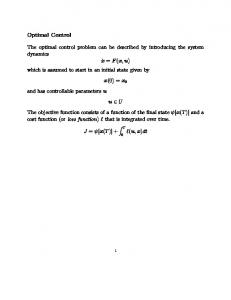
17 Proof. The proof is standard. Assuming optimality beyond the intersecting point, we can construct a broken minimizer which is an extremal of order 0 with non-zero pθ . This contradicts proposition 5.8. 5.2.3. Numerical computations. We complete the analysis of section 5 by a series of numerical computations on extremal trajectories and on conjugate loci (see section 2). All the computations are done in the case of the time-minimum control problem but could be equivalently done for the energy minimization problem. We use numerical methods described in [6]. Extremal trajectories: We compute extremal trajectories for different values of the dissipative parameters Γ and γ+ . We represent in figures 5.1 and 5.2 in the coordinates (θ, φ) the projection of the trajectories on the sphere of radius 1. The variation of the radial coordinate ρ can be deduced straightforwardly and depends on the value of Γ and γ+ . Extremals can also be plotted in the plane (φ, pφ ) by using equation (5.1). In figure 5.1, two trajectories intersecting with the same cost on the antipodal parallel are plotted. All other extremal trajectories in the case |Γ−γ+ | < 2 are qualitatively the same behavior. For the Grusin model on the sphere, we also recall that the two trajectories which intersect on the cut locus have opposite initial values of pφ , ε and pθ being fixed. This is no more the case when Γ 6= γ+ since these initial values depend now on Γ and γ+ . The extremal trajectories for |Γ − γ+ | > 2 are displayed in figure 5.2. We observe two types of trajectories, the periodic and the aperiodic ones. The periodic extremals have the same behavior as the ones of the case |Γ − γ+ | < 2. When t → +∞, the aperiodic extremals have an asymptotic limit φS in φ solution of the equation (5.10). For given values of pθ and ε, this equation has two solutions symmetric with respect to the equator. As can be seen in figure 5.2, we have found two types of aperiodic extremals: trajectories monotone in φ which do not cross the parallel φ = φS and trajectories passing by a maximum or a minimum in φ different from φS and crossing this parallel. These different types of behaviors can be determined by using equations (5.6) and (5.7). Conjugate locus: 3

2.5

φ

2

1.5

1

0.5

0 0

0.5

1

1.5

2

θ

2.5

3

3.5

4

Fig. 5.1. Extremal trajectories for Γ = 2.5 and γ+ = 2. Other parameters are taken to be pφ (0) = −1 and 2.33, φ(0) = π/4, pr = 1 and pθ = 2. Dashed lines represent the equator and the antipodal parallel located at φ = 3π/4.

18 3

2.5

φ

2

1.5

1

0.5

0 0

0.5

1

1.5

θ

2

2.5

3

Fig. 5.2. Extremal trajectories for Γ = 4.5 and γ+ = 2. Dashed lines represent the equator and the locus of the fixed points of the dynamics given by equation (5.10). The solid line corresponds to the antipodal parallel. Numerical values of the parameters are taken to be φ(0) = 2π/5, pθ = 2 and pr (0) = 1.

We next determine numerically the conjugate locus for different set of parameters. We restrict the discussion to the case |Γ − γ+ | < 2. A similar study can be done for periodic trajectories if |Γ − γ+ | ≥ 2. For aperiodic trajectories, it can be shown that they are locally optimal in the sense that they do not have conjugate points for t ∈ [0, +∞[. Different conjugate loci are represented in figures 5.3, 5.4 and 5.5 both for the Grusin model and for a deformation of this model with the constraint |Γ − γ+ | < 2. The conjugate locus of the Grusin model on the sphere is given in [4]. Here, in the case Γ = γ+ , the drift vector F0 being purely radial, the projection of the conjugate locus is the same as the conjugate locus of the Grusin model on the sphere. In particular, this projection is independent of the value of pr . Figure 5.3 displays both this conjugate locus and some extremal trajectories. Starting from the Grusin model, we can then modify the difference Γ − γ+ and determine the corresponding deformation of the conjugate locus. The evolution of the radial component being more complicated (the radial coordinate is no more decoupled from other coordinates if Γ 6= γ+ ), the projection of the conjugate locus depends on the value of pr . A first comparison between the two cases is given by figure 5.4 where it can be seen that the global structure of the extremals is nearly the same. Figure 5.5 displays the projection of a conjugate locus on the plane (θ, φ) corresponding to a particular value of pr . The conjugate locus of the Grusin model has been added for the sake of comparison. We note that this locus is only slightly modified when Γ and γ+ vary. REFERENCES [1] C. Altafini, Controllability properties for finite dimensional quantum Markovian master equations, J. Math. Phys. 44, 2357-2372 (2002). [2] A. Agrachev, U. Boscain and M. Sigalotti, A Gauss-Bonnet like formula on twodimensional almost Riemannian manifolds, Preprint Sissa 55, Trieste (2006). [3] D. Bao, C. Robles and Z. Shen, Zermelo navigation on Riemannian manifolds, J. Differential Geom. 66 (2004), n3, 377-435. [4] B. Bonnard and J.-B. Caillau, Riemannian metric of the averaged energy minimization problem in orbital transfer with low thrust, Ann. Inst. Henri Poincar´ e (Analyse non lin´ eaire)

19 3

2.5

φ

2

1.5

1

0.5

0 0

0.5

1

1.5

θ

2

2.5

3

Fig. 5.3. Extremal trajectories for the Grusin model corresponding to Γ = γ+ = 2. The conjugate and cut loci are represented in dashed lines.

3

2.5

φ

2

1.5

1

0.5

0 0

0.5

1

1.5

2

θ

2.5

3

3.5

4

Fig. 5.4. Extremal trajectories for Γ = 2.5 and γ+ = 2. The projection of conjugate locus is represented in dashed lines. The horizontal dashed line is the line where two trajectories intersect with the same length. Numerical values for the parameters are taken to be φ(0) = π/4, pr = 1 and pθ = 1.

24, 395-411 (2007) [5] B. Bonnard, J-B. Caillau, R. Sinclair and M. Tanaka, Conjugate and cut loci of a two-sphere of revolution with application to optimal control, submitted to Ann. Inst. H. Poincar´ e (2008). ´lat, Second-order optimality conditions in the smooth [6] B. Bonnard, J-B Caillau and E. Tre case and applications in optimal control, ESAIM : COC V 13, no. 2, 207-236 (2007) [7] B. Bonnard and M. Chyba, Singular trajectories and their role in control theory, Math. and Applications 40, Springer-Verlag, Berlin (2003) [8] B. Bonnard and D. Sugny, Optimal control theory with applications in space and quantum dynamics, submitted (2008). [9] U. Boscain, T. Chambrion and J-P. Gauthier, On the K + P problem for a three-level quantum system: Optimality implies resonance, J. Dyn. and Control Syst. 8, 547-572 (2002)

20 3

2.5

2

1.5

1

0.5

0 0

0.5

1

1.5

2

2.5

3

3.5

4

Fig. 5.5. Projection of conjugate locus in solid line for pr = 1. The conjugate locus of the Grusin model corresponding to γ+ = Γ = 2 is represented in dashed lines. The horizontal dashed line indicates the position of the cut locus for the Grusin model. Dissipative parameters are taken to be Γ = 2.5 and γ+ = 2, pθ is equal to 1.

´rin and H. R. Jauslin, Optimal control in [10] U. Boscain, G. Charlot, J-P. Gauthier, S. Gue laser induced population transfer for two and three-level quantum systems, J. Math. Phys. 43, 2107-2132 (2002) [11] U. Boscain and B. Piccoli, Optimal syntheses for control systems on 2-D manifolds, SpringerVerlag, Berlin (2003). ´odory, Calculus of variations and partial differential equations of first order, [12] C. Carathe Chelsea Publishing Company, New-York (1982). [13] E. Lee and L. Markus, Foundations of optimal control theory, John Wiley, New York 1967. [14] S. G. Schirmer and T. Zhang and J. V. Leahy, Orbits of quantum states and geometry of Bloch vectors for N-level systems, J. Phys. A, 37, 1389-1402 (2004). [15] D. Sugny, C. Kontz and H. R. Jauslin, Time-optimal control of a two-level dissipative quantum system, Phys. Rev. A, 76, 023419 (2007).