Oct 6, 2011 - Ting Heâ¡. AbstractâWe consider an online preemptive scheduling prob- lem where jobs with deadlines arrive sporadically. A commitment.
Optimal Deadline Scheduling with Commitment
arXiv:1110.1124v1 [cs.DS] 6 Oct 2011
Shiyao Chen†
Lang Tong†
Abstract—We consider an online preemptive scheduling problem where jobs with deadlines arrive sporadically. A commitment requirement is imposed such that the scheduler has to either accept or decline a job immediately upon arrival. The scheduler’s decision to accept an arriving job constitutes a contract with the customer; if the accepted job is not completed by its deadline as promised, the scheduler loses the value of the corresponding job and has to pay an additional penalty depending on the amount of unfinished workload. The objective of the online scheduler is to maximize the overall profit, i.e., the total value of the admitted jobs completed before their deadlines less the penalty paid for the admitted jobs that miss their deadlines. √ We show that the maximum competitive ratio is 3 − 2 2 and propose a simple online algorithm to achieve this competitive ratio. The optimal scheduling includes a threshold admission and a greedy scheduling policies. The proposed algorithm has direct applications to the charging of plug-in hybrid electrical vehicles (PHEV) at garages or parking lots. Index Terms—Deadline scheduling; competitive ratio analysis; commitment requirement; PHEV charging scheduling.
I. I NTRODUCTION In a conventional setting of deadline scheduling, jobs arrive sporadically, each with prescribed processing time, deadline, and value. Upon arrival, jobs are queued until their respective deadlines, during which time an online scheduler can schedule any pending jobs in the system. In general, there is no guarantee that a submitted job will be completed by its deadline. In fact, a customer who submits a job does not know whether the job will be completed until after the deadline. For example, an online scheduler may accept a job into the system but later choose to work on another more profitable job instead. In this paper, we consider a variation of the deadline scheduling problem by imposing a commitment requirement at the arrival of a job. In particular, if a job is accepted and successfully completed, the scheduler receives a certain reward. If the scheduler is unable to complete an accepted job, it pays a penalty. The scheduler receives neither reward nor penalty if it declines a job upon arrival. The deadline scheduling problem considered in this paper has a direct application in scheduling the charging of plug-in hybrid electric vehicles (PHEV) in parking lots or garages. In this case, each car arrives with a certain charge level, and the customer has some idea about how long the car can be left at the facility (e.g., approximately the duration in which the customer will be shopping before picking up the car). Upon submitting a request, the customer is either turned away or told † School
of ECE, Cornell University, Ithaca NY 14853. T.J. Watson Research Center, Hawthorne, NY 10532. This research was sponsored in part by the U.S. National Institute of Standards and Technology under Agreement Number 60NANB10D003 and the National Science Foundation under a Grant CNS-1135844. ‡ IBM
Ting He‡
the car will be charged at a certain price. And the customer is informed that if the car is not charged to the requested level by the deadline, a compensation will be made (e.g., with a voucher for future charges). While the requirement of immediate commitment reduces the number of unsatisfactory customers and the amount of penalty, it brings nontrivial complications to the deadline scheduling problem. The difficulty comes from the fact that optimal decision on whether to turn away a customer seems to depend on the kind of jobs to arrive in the future. Had the scheduler known that there is a highly profitable job to arrive, it would have declined some of the less profitable ones. Our goal is to maximize the profit by optimally trading off accepting more customers against avoiding excessive penalties due to unfinished jobs. To accommodate general arrivals and workload, we aim at optimizing the competitive ratio that characterizes the worst-case profit relative to that of an optimal offline scheduling algorithm, for which we establish the optimal competitive ratio and give an online scheduling algorithm to achieve the optimum competitive ratio. A. Related Work Without the commitment requirement, there is a considerable literature on the deadline scheduling problem, starting from the seminal work of Liu and Layland [1]. The problem is often divided into the underloaded and overloaded regimes. The former corresponds to the case when there exists an offline scheduling algorithm that can complete all jobs arrived whereas the latter corresponds to the case when some jobs cannot be completed even for the best offline scheduling algorithm. For the underloaded scenarios, it has been shown that simple online scheduling algorithms such as earliest deadline first (EDF) [1], [2] and least laxity first (LLF) [3] achieve the same performance as the optimal offline scheduling algorithm. The assumption of underloaded overall workload, however, is restrictive and unverifiable in practice. Locke showed in [4] that both EDF and LLF can perform poorly in the presence of overload. There were efforts to develop an online scheduling algorithm with performance guarantee in terms of competitive ratio (see Definition 1), even when the system is overloaded. Online scheduling algorithms with competitive ratio 1/4 were proposed in [5], [6] and 1/4 was proved to be optimal competitive-ratio-wise for the deadline scheduling problem without commitment. One of the first work that proposes the idea of commitment is [7] (commitment is termed as immediate notification), in which Bar-Noy et. al. considered the application of video on demand where customers submit movie request and the scheduler manages to either accept or decline the request within
a specific “notification time” after the request releases. BarNoy et. al. studied the competitive ratio when the “notification time” varies from zero (immediate notification) to proportional to the length of the movie requested. Later, scheduling with immediate notification and immediate decision has been studied in [8] (single processor, immediate notification), [9] (multiple processors, immediate notification), and [10], [11] (multiple processors, immediate decision). Immediate decision requires that, in addition to providing to the customers an immediate feedback regarding admission or declination, the scheduler also has to provide to the customer upon job release the specific scheduled time of the job, if accepted. The proportional value model was considered in [8], while [10], [9] considered the unit length jobs with unit value. An online scheduling algorithm with immediate decision is proposed in [10] with asymptotic competitive ratio (e − 1)/e, while the authors of [11] showed (e − 1)/e to be an asymptotic upper bound of any online algorithms. However, the authors of [8], [9], [10], [11] dealt with non-preemptive scheduling with no non-completion penalty involved. With the commitment requirement online preemptive scheduling with deadlines becomes much more challenging in the presence of overload. The authors of [12] and the author of [13] gave separately two preemptive scheduling algorithms for multiple processors with immediate notification and non-completion penalty with the proportional value model (vi = pi , see Section II). In [12], [13] the non-completion penalty associated with a job with value vi = pi is set as ρvi with the penalty parameter ρ ≥ 0. The competitive ratio results given in [12], [13] arep(mina>1+ρ (2a + 3)(1 + ρ 1 −1 and (2ρ + 3 + 2 ρ2 + 3ρ + 2)−1 , respeca−ρ + a−ρ−1 )) tively. Even for the situation with no non-completion penalty (ρ = 0), the competitive ratio results given in [12], √ [13] 1 reduces to (mina>1 (2a + 3)(1 + a−1 ))−1 = (7 + 2 10)−1 √ and (3 + 2 2)−1√, respectively, which is at most as good as our result 3 − 2 2 in this paper for single processor with non-completed portion penalized. On the other hand, there are no arguments in [12], [13] establishing upper bounds of competitive ratio ever achievable to quantify how far the proposed algorithms are away from optimality. There is a series of work by Hou, Borkar and Kumar [14], [15], [16] and Jaramillo, Srikant and Ying [17], [18] dealing with the deadline scheduling problem with a different setup from that adopted in this paper. Specifically, the channel (the counterpart in [14], [15], [16], [17], [18] of the processor in this paper) is modeled as a stationary, irreducible Markov process with a finite state space (unreliable channel model), whereas the processor is always dedicated to scheduling the jobs in this paper. Due to the unreliable channel model, the packet transmission (the counterpart of the job in this paper) may take a random amount of time to go through, whereas the job length in this paper is deterministic upon arrival. Each client (transmitter) specifies a delay requirement (transmissions which take longer than the delay requirement is invalid), which corresponds to the deadlines in this paper. The
packet arrival process is assumed to be a stationary, irreducible Markov process with finite state space for each client, whereas the job arrival process can be arbitrary and quite bursty in this paper. Thus, the stochastic model of the processor (channel), the job (packet) arrival process and the job length (packet transmission duration) is available in [14], [15], [16], [17], [18]. On the other hand, the job arrival as well as the job length can be arbitrary for the future job released in this paper. There is also difference in the metric used; the feasibility optimality is studied in [14], [15], [16], [17], [18], i.e., the overall packet arrival is assumed to be underloaded, whereas the overloaded scenario is treated in this paper with the metric competitive ratio. The problem of PHEV charging scheduling in public garage has been considered in [19], [20], [21]. An energy economic analysis of PHEV charging using solar photovoltaic panels at workplace parking garage is conducted in [20] with the conclusion that PHEV charging facility in public garage is beneficial to both the car owners as well as the facility operator. The authors of [19] aggregated a system architecture model, an operation model and a PHEV battery model to simulate PHEV charging in a municipal parking lot. The method of particle swarm optimization is employed to allocate energy to PHEVs in [21]. The performance of the scheduling policies proposed in [19], [20], [21] are validated via simulation results. This paper adopts a deadline scheduling framework with non-completion penalty that suits well for PHEV charging application and proposes an online scheduling algorithm with worst case performance guarantee. B. Summary of Results In this paper, we impose a penalty on unfinished workload and obtain results on the optimal competitive ratio for the online preemptive deadline scheduling with commitment. We propose an online scheduling algorithm DSC (acronym for Deadline√Scheduling with Commitment) with competitive ratio 3 − 2 2 = 17.16%. We also provide a converse via an adversary argument and show that no online scheduling algorithm exists with a better competitive ratio, thus further establishing the optimality of DSC competitive-ratio-wise. Comparing with the optimal competitive ratio 1/4 = 25% without the commitment requirement in [5], [6], we observe a performance loss of 7.84% competitive-ratio-wise with the additional commitment obligation. II. P ROBLEM F ORMULATION A job T = (r, p, d, v) is represented by a quadruple specified by the release time r, processing time p, deadline d, and value v. We assume the so-called proportional value model [8] where the value v of a job is proportional to its processing time p, or without loss of generality, v = p. A job T is called tight if r + p = d, which implies that the scheduler must either work on the job or decline it immediately. Preemption is allowed at no cost in scheduling (i.e., a preempted job can be resumed from the point of preemption at a later time). In our scheduling problem an input instance I includes n jobs
T1 , . . . , Tn to be scheduled on a single processor, where the integer n is the total number of jobs released for instance I (the total number of jobs can differ over input instances). In general, we are interested in a collection of instances in the input instance set I. Use Sonline to denote online scheduler and Soffline the offline scheduler. An online scheduler Sonline knows the parameters of job Ti only at the release time ri . Deadlines are firm, i.e., completing a job after its deadline yields zero value. The scheduling is done with commitment, i.e., upon the release of each job, the scheduler has to decide whether to accept or decline the job request. Each accepted job incurs a non-completion penalty equal to the unfinished workload (shortage) if it is not completed by its deadline. The profit obtained by the scheduler is the total value of all completed jobs, minus all penalties paid. This specific non-completion penalty suits the application of PHEV charging well since the utility is delivered to the car owner continuously as the battery charging level increases, unlike some computing jobs in high performance computing grids for which the utility can be obtained only upon the completion of all the computation steps. Given an instance I, we denote by Sonline (I) (Soffline (I)) as the total profit (or value) obtained by the scheduler Sonline (Soffline ). Our objective is to make the online scheduler competitive across all instances in I. In contrast to the online scheduler, an offline scheduler Soffline is clairvoyant and knows the entire input instance a priori. Due to the prior knowledge of the job parameters, the offline scheduler is able to make commitment decisions. We denote ∗ by Soffline the optimal offline scheduler. The problem is to design an online scheduling algorithm with worst-case performance guarantee (relative to the optimal offline scheduling algorithm) even in the presence of overload. The performance guarantee is given in terms of competitive ratio defined below. Definition 1. Competitive ratio: An online algorithm Sonline is (I) ≥ α-competitive for an input instance set I if minI∈I SSonline ∗ offline (I) α where I varies over all possible input instances in I. That is, an α-competitive online algorithm is guaranteed to achieve at least α fraction of the optimal offline value under any input instance I in the input instance set I. For the rest of the paper the input instance set I is fixed to be the set of all input instances I such that I contains finite number of jobs and each job satisfies di ≥ ri + pi (otherwise, neither the online nor the offline scheduler is able to complete the job by its deadline and the job can thus be deleted from the input instance I). Note that both underloaded and overloaded input instances are included in the input instance set I defined above. III. O PTIMAL D EADLINE S CHEDULING C OMMITMENT
WITH
Compared with the traditional deadline scheduling without the commitment requirement, the additional difficulty imposed
by the commitment obligation to the online scheduler depends on the overall workload of the jobs released: when the overall workload is underloaded, simple scheduling algorithms such as EDF and LLF achieve competitive ratio 1 by simply admitting all jobs released; the restriction to the underloaded case precludes the need of admission control. In this section, we describe an online scheduling algorithm DSC dealing with the overloaded scenario and establish √its optimality in competitive ratio. Specifically, we show 3−2 2 as the optimal worst-case performance of online algorithms relative to the (optimal) offline counterpart. We summarize these results in the following theorem followed by a detailed description of DSC. Theorem 1. For the input instance set I specified in Section II, √ 1) The competitive ratio 3 − 2 2 is achievable by DSC. √ 2) 3 − 2 2 upper bounds the competitive ratio ever achievable by any online scheduling algorithms. In other words, there is a loss of 7.84% competitive-ratiowise with the additional commitment obligation when we compare the optimal competitive ratio 1/4 = 25% without the commitment √ requirement ([5], [6]) with the result in Theorem 1 (3 − 2 2 = 17.16%). A. DSC Scheduling Algorithm The key idea behind DSC is to evaluate the admission decision based on the comparison of the potential profit associated with accepting and declining a job, if the job is “difficult” to accommodate into the current schedule. Even assuming the scheduler accepts the job just released, there are plenty of alternatives in the specific schedule of the job just released as well as the other pending jobs in the system (due to the acceptance of the new job, it may be necessary to update the schedule of the other jobs). DSC evaluates the profits associated with the two options by restricting to one alternative in the many ways of updating of the schedule after accepting the newly released job. Specifically, if the newly released job can be appended in the end of the current schedule while still being within its deadline (the job is “easy” to accommodate into the current schedule, see the blue, green and red jobs in Fig. 1, Fig. 2 and Fig. 6, respectively for illustration), the job is accepted and appended in the end of the current schedule. Otherwise (the job is “difficult” to accommodate into the current schedule, see the green and brown jobs in Fig. 3 and Fig. 7, respectively for illustration), the two options are weighed separately, described in detail in later paragraphs. If the option of accepting the job is chosen, the schedule is updated by tight-scheduling the newly released job in the interval [d − p, d] where p and d are the processing time and deadline of the newly released job, respectively. Then the part of the previous schedule after time d − p is moved to start at time d, or the end of the current schedule, whichever comes later in time (see the red job in Fig. 8 for illustration). This moving may lead to some of the moved jobs to miss their deadlines. Therefore the schedule is again updated to remove
the part of the moved jobs that comes after their deadlines. The decision process can be interpreted as follows. When the scheduler decides to accept the newly released job, the job is profitable once accepted but difficult to accommodate into the current schedule. Therefore in order to accommodate the newly released profitable job, the scheduler sacrifices the jobs in the current schedule in the time interval [d − p, d], some of which may have deadlines far into the future, thus still have potential in completion even after the moving. To give the procedure to compute the profit associated with the two options, we first define the notions of peace-scheduled and contention-scheduled jobs. We term a job peace-scheduled if it is scheduled without affecting other already scheduled jobs (by the appendable statement on line 4), and contentionscheduled if it is scheduled with moving some already admitted and unfinished jobs to a later time (by the not appendable statement on line 6 to 10). In between two consecutive admission decisions of contention-scheduled jobs, all the jobs are peace-scheduled and the accepted jobs are always appended in the end of the schedule. The procedure to determine the profit for accepting and declining the jobs that cannot be appended can be described as follows. First execute (virtually) on the current tentative schedule the procedure associated with the decision to accept the difficult-to-accommodate job (including scheduling the newly released job in [d−p, d] and postponing the previous jobs in [d − p, d]) and find out the jobs in the current tentative schedule that are affected in the received processing time. Denote by Jaffect the set of jobs in the current tentative schedule that are affected in the received processing time. The profit associated with the option of declining can be computed as the value of the subset of jobs in Jaffect anticipated to complete by the current tentative schedule, less the portion of penalty attributed to the subset of jobs. The profit associated with the option of accepting can be computed as the value of the newly released job, less the portion of penalty attributed to the acceptance of the newly released job (due to affecting the jobs in Jaffect ). See Fig. 4, Fig. 5, Fig. 8 and Fig. 9 for illustration of the profits and the decision after comparing the profits. Fig. 10 depicts the final schedule of this instance. To summarize, the dynamics of the system with DSC scheduler can be described as follows: the scheduler maintains a tentative schedule at all times; when a job request is released, the scheduler checks whether it is possible to append the new job at the end of the current tentative schedule while meeting its deadline. If the deadline can be met, then the job is admitted and appended in the end of the current tentative schedule. Otherwise, the scheduler determines whether to admit the job based on the profits of the options of accepting and declining. If the profit associated with accepting is not sufficiently large, then the job is simply declined service. Otherwise, the job is scheduled in the time interval [di − pi , di ]; the previous schedule after time di − pi is then moved to start at time di , or the end of the current schedule, whichever comes later in time, and the scheduler further checks whether there are any moved jobs that already missed their deadlines after the
t Figure 1.
moving, deletes them and moves the jobs accordingly to fill the gap left by the jobs deleted. We now describe the details of the DSC algorithm. The pseudo code of DSC is given below. At time 0 the scheduler starts the infinite loop in which the schedule is updated upon each job release. DSC Scheduling Algorithm procedure 1: loop 2: upon event: job Tarr is released 3: if Tarr appendable then 4: append Tarr to the end of the tentative schedule; 5: else 6: if Profitaccept > (1 + β)Profitdecline then 7: append Tarr at the end by darr 8: move and modify the schedule after darr − parr accordingly 9: else 10: decline Tarr 11: end if 12: end if 13: end loop As indicated in the algorithm pseudo code Tarr gets admitted and appended to the current schedule if it is appendable (line 4). Otherwise, the profits Profitaccept and Profitdecline associated with admitting and declining Tarr respectively get compared. If admitting Tarr assumes better profit (line 6), then Tarr is admitted and appended at the end by darr (i.e., scheduled in the time interval [darr − parr , darr ]), and the current schedule after darr − parr is moved and modified accordingly (line 7 and 8). Otherwise, if admitting Tarr does not have better profit, Tarr is declined service (line 10). The threshold 1 + β will be optimized after we derive the competitive ratio as a function of β (see Section III-D). The appendable case takes O(1) per job. while the non-appendable case takes O(n) per job, where n is the number of jobs in the current schedule. We state the differences between the DSC algorithm and the algorithms in [5], [6] for the situation without commitment: the contention of the processor is resolved using the profit (i.e., job values minus penalties) instead of the job value alone. B. Analyzing the Structure of DSC Algorithm Denote a continuous busy interval (a continuous time interval in which the processor is busy executing jobs) by B = [t, t]. We start the analysis of the structure of DSC
t Figure 9.
Figure 2.
Figure 10. Figure 3.
Figure 4.
Figure 5.
algorithm by classifying the continuous busy intervals created by the execution of DSC into two different types with different structures. The first type busy interval corresponds to the situation where there is no processing time corresponding to contention-scheduled jobs. In this case, all jobs admitted are peace-scheduled and finish successfully by t, the time at which the processor finishes the tentative schedule and gets idle. The second type busy interval corresponds to the situation where there are some contention-scheduled jobs inside the continuous busy interval. Denote by TB , PB and CB the total profit obtained in schedule from all jobs, from peace-scheduled jobs and from contention-scheduled jobs during B, respectively. Note that the penalty is included in the profit TB and CB . For every continuous busy interval B it holds that TB = PB + CB .
Figure 6.
(1)
Denote by B the union of all continuous busy intervals. The length of B will be denoted by |B|. We refer to its total, peace-scheduled and contention-scheduled value obtained in schedule by T, P and C, respectively. Lemma 1 upper bounds the total processing time in a continuous busy interval B with TB , PB and CB . Lemma 1. The total processing time of B = [t, t] satisfies |B| ≤ PB + (1 +
Figure 7.
1 1 )CB = TB + CB . β−1 β−1
(2)
Lemma 2 upper bounds the deadlines of the jobs that are declined during the continuous busy interval B. Note that there are no jobs declined when the processor is idle under DSC algorithm. Lemma 2. Suppose Ti was declined during the continuous busy interval B = [t, t]. Then X sj ≤ (1 + β)TB , di − t − rj ∈B
Figure 8.
where sj is the shortage (at time t) of job Tj that is admitted in B (rj ∈ B).
Lemma 3 provides a useful fact for the peace-scheduled jobs that eventually fail. Lemma 3. Suppose Ti ’s are peace-scheduled jobs that eventually failed. Then Ti ’s are such that [ri , di ] ⊂ B. Proof: If Ti is peace-scheduled at time ri , then Ti is included in the schedule since time ri . Assume that [ri , di ] ⊂ B does not hold. Therefore there exists time instant τ ∈ [ri , di ] such that the processor is idle at time τ . However, this contradicts the way the DSC algorithm runs due to the following argument. At time τ Ti is not finished yet because Ti failed eventually. Therefore the scheduler can work on Ti at time τ in the tentative schedule either with the goal of completing Ti for its value or with the goal of reducing the penalty associated with Ti . Thus either way the processor should be busy, contradicting the assumed fact that the processor is idle at time τ . This contradiction proves [ri , di ] ⊂ B. C. Upper Bounding Optimal Offline Value Given a collection of jobs I, denote the optimal value that an offline algorithm can obtain from scheduling the set of jobs I ∗ ∗ by Soffline (I). We derive an upper bound of Soffline (I) for I being the set of released jobs. We partition the collection of jobs I = S c ∪S p ∪F p ∪F c ∪D where S c (S p ) denotes the successful contention-scheduled (peace-scheduled) jobs, F c (F p ) denotes the failed contention-scheduled (peace-scheduled) jobs and D the declined jobs under DSC algorithm. ∗ ∗ ∗ Since Soffline (S c ∪S p ∪F p ∪F c ∪D) ≤ Soffline (S p )+Soffline (S c ∪ c p F ∪ F ∪ D), we upper bound the two terms separately. ∗ We upper bound the term Soffline (S c ∪ F p ∪ F c ∪ D) by considering the optimal offline algorithm for S c ∪F p ∪F c ∪D under a processing-time-granted-value setting. (The grantedvalue setting is first used in [6] to treat the no commitment case.) Specifically, the offline scheduler receives an additional granted value besides the value obtained from S c ∪F c ∪F p ∪D. The amount of granted value depends on the offline schedule: unit value will be granted for unit processing time in B that is not used for executing jobs in S c ∪ F p ∪ F c ∪ D. Under the granted-value setting the optimal offline scheduler must consider that scheduling a job might reduce the granted value (since processing time in B is used). Executing a job Ti results in a gain of vi and a loss of the granted value for the processing time of Ti that is executed in B. One offline schedule under the granted-value setting is to schedule no jobs in S c ∪ F p ∪ F c ∪ D (therefore leaving the entire B period untouched) and get only the (whole) granted value. This scheduling-nothing schedule obtains a value of |B|. Since Lemma 1 upper bounds the total processing time in a continuous busy interval, we can upper bound the total processing time in B, and thus the value obtained by the scheduling-nothing schedule. However, the optimal offline schedule under the grantedvalue setting may use some processing time of B to schedule certain jobs in S c ∪ F p ∪ F c ∪ D to obtain more value than the ∗ scheduling-nothing schedule. To upper bound Soffline (S c ∪ F p ∪ c F ∪ D) under the granted-value setting, we take the value
of the scheduling-nothing schedule as a benchmark and turn to upper bounding the net gain the optimal schedule can have over the scheduling-nothing schedule by completing some jobs in S c ∪ F p ∪ F c ∪ D. We first observe that any job Ti ∈ F c ∪ S c will be such that [ri , di ] ⊂ B, since at the time ri , Ti is contention-scheduled in the interval [di − pi , di ]. Therefore the busy period covers [ri , di ]. We also observe by Lemma 3 that a peace-scheduled job Tf ∈ F p which eventually fails also satisfies [ri , di ] ⊂ B. By the definition of the granted value we can see that under the optimal offline algorithm, no job is scheduled entirely in B because the granted value lost would be equal to the value of the job. Therefore the optimal offline schedule will not choose to schedule any jobs in S c ∪ F p ∪ F c . Since we are interested in scheduling jobs in S c ∪ F p ∪ c F ∪ D such that only small amount of B processing time is used (thus small loss of granted value), we leverage the fact that when a job Td ∈ D is declined during busy interval B, the deadline of Td can not be too far with respect to the end of B, given by Lemma 2. Lemma 4 provides the earliest time for an offline scheduler to execute a job in D outside B. Lemma 4. Suppose Td ∈ D is declined by the online scheduler at time rd and rd ∈ B = [t, t]. Then, if Td is to be executed by the offline scheduler anywhere outside B it must be after t. Proof: The proof can be easily done using the fact rd ∈ B = [t, t], leading to [rd , t] ⊂ B. Lemma 5 upper bounds the net gain the optimal offline scheduler will obtain over the scheduling-nothing benchmark, restricted to the jobs that are declined during B. Lemma 5. Under the granted-value setting the total net gain obtained by the offline algorithm from scheduling the jobs in S c ∪ F p ∪ F cP ∪ D released in B = [t, t] is no greater than (1 + β)TB + rj ∈B sj . Proof: According to Lemma 2 if Ti was declined during the busy interval B = [t, t]. Then X sj , di − t ≤ (1 + β)TB + rj ∈B
where sj is the shortage (at time t) of job Tj that is admitted in B and the summation of rj ∈ B is summing over all jobs Tj that are admitted in B. On the other hand under the granted-value setting the net gain obtained by the offline algorithm from scheduling the jobs in S c ∪ F p ∪ F c ∪ D released in B = [t, t] can only come from D and the earliest time Td can be executed by the offline scheduler outside B is t. Therefore the net gain obtained by the offline algorithm from scheduling the jobs in S c ∪ F p ∪ F c ∪ D in B = [t, t] is bounded by X sj , max di − t ≤ (1 + β)TB + Ti ∈DB
rj ∈B
where DB is the subset of D released in B.
Lemma 6 upper bounds the total shortage t). Lemma 6.
P
rj ∈B
P
rj ∈B
sj (at time
sj ≤ |B| − TB .
Proof: P Since each Tj that is not finished in B contributes sj to rj ∈B sj and −s Pj to TB , and each Tj that is finished in B contributes 0 to rj ∈B sj , vj to TB and vj to |B|, the lemma is proved. D. Proving Theorem 1 We now prove Theorem 1 after bounding the net gain of scheduling the jobs in S c ∪ F p ∪ F c ∪ D. Proof: Lemma 5 bounds the maximum net gain for each busy interval. By construction, each job is accounted for in exactly one continuous busy interval. Therefore, summing over all busy intervals we conclude using Lemma 6 that under the granted value setting the total net gain during the entire execution horizon obtained by the offline algorithm from scheduling the jobs of S c ∪F p ∪F c ∪D is bounded by |B|+βT, where B is the union of all the busy intervals. Combining the upper bound of the total net gain and the value of the scheduling-nothing benchmark, i.e., the processing time in B, yields ∗ Soffline (I) ≤
≤ ≤ ≤ ≤ ≤
≤
∗ ∗ (S p ) (S c ∪ F p ∪ F c ∪ D) + Soffline Soffline
|B| + (|B| + βT) + value(S p ) 2|B| + βT + value(S p ) 2 C+P (β + 2)T + β−1 2 2 C+ P (β + 2)T + β−1 β−1 2 (β + 2 + )T β−1 √ (3 + 2 2)T,
(3) (4)
(5)
where Eq. (3) is obtained from summing Lemma 1 over all continuous busy intervals, Eq. (4) holds when β ≤ 3, and Eq. √ (5) is obtained by optimizing over β, which yields β = 1+ 2 and √ ∗ (6) Soffline (I) ≤ (3 + 2 2)T, where I = S p ∪ S c ∪ F p ∪ F c ∪ D is the set of released jobs. Since the value of the optimal offline schedule is at most ∗ Soffline (I) and the profit √ obtained by DSC algorithm is T, the competitive ratio 3 − 2 2 is shown to be achievable by DSC algorithm. IV. U PPER B OUND
ON
C OMPETITIVE R ATIO
An adversary argument establishes the upper bound on the competitive ratio ever achievable by any online scheduler. Specifically, we construct a job input instance I, such that the competitive ratio for√ the constructed job input instance is upper bounded by 3 − 2 2. Consider the input instance I constructed by the adversary which contains a sequence of tight jobs (ri + pi = di ). The first tight job T0 is released at time 0 with processing length
x0 = 1. The offline adversary observes the action of the online scheduler and then decides future job releases. Upon the release of T0 the online scheduler can choose either to admit or to decline the job T0 . If declined, the offline adversary will choose to release no more jobs and eventually the offline adversary obtains x0 while the online scheduler 0. If admitted, the adversary will choose to release another tight job T1 at time ǫ, with processing length x1 . Then similarly the online scheduler can choose either to admit or to decline the job T1 upon arrival. Similarly, if declined, the offline adversary will choose to release no more jobs and eventually the offline adversary obtains x1 while the online scheduler x0 . If admitted, the adversary released another tight job T2 at time 2ǫ, with processing length x2 . The whole process keeps going until the online scheduler chooses to decline the first job in the process. For the (n+2)th release the offline adversary releases the tight job Tn+1 at time (n + 1)ǫ, with processing length xn+1 . Then similarly the online scheduler can choose either to admit or to decline the job Tn+1 upon arrival. If declined, the offline adversary will choose to release no more jobs and eventually the offline Pn−1 xn+1 Pn−1adversary obtains while the online scheduler xn − j=0 xj , where j=0 xj is the non-completion penalty paid by the online scheduler (the non-completion penalty should ideally include a term with ǫ, however, the adversary will choose ǫ to be arbitrarily small and the term can be left out in the following derivation). For the above job release up to Tm+1 (i.e., even the online scheduler chooses to admit up to job Tm+1 , the offline adversary will not release new jobs), the competitive ratio ever achievable for the above constructed input instance is Pm xm+1 − j=0 xj max{σ1 , σ2 , . . . , σn+1 , . . . , σm+1 , }, (7) xm+1 xi −
Pi−1
xj
j=0 , for i = 0, 1, . . . , m. where σi+1 = xi+1 Now we design the processing lengths xi to upper bound the value of Eq. (7). We first set all terms but the last inside the minimum in Eq. (7) to be 1/c.
cx0
= x1
c(x1 − x0 )
= x2 .. .
c(xn − c(xn+1 −
n−1 X
xj )
= xn+1
(8)
j=0 n X
xj )
= xn+2
(9)
j=0
.. . c(xm −
m−1 X j=0
xj )
= xm+1
We can then obtain the recursion by subtracting Eq. (8) from Eq. (9), x0 = 1,
x1 = c,
c(xn+1 − 2xn ) = xn+2 − xn+1 , (10)
with the characteristic function x2 − (c + 1)x + 2c = 0.
(11)
We still need the last term inside the maximum in Eq. (7) to be no greater than 1/c, P xm+1 − m 1 j=0 xj ≤ . (12) xm+1 c Rewrite Eq. (12) to be P xm+1 − m j=0 xj xm+1
≤
xm −
Pm−1 j=0
xm+1
xj
,
(13)
which implies xm+1 ≤ 2xm ,
(14)
and further (due to Eq. (10)) xm+2 ≤ xm+1 . (15) √ For any 1 ≤ c < 3 + 2 2 the characteristic function has two complex roots and there exists m such that Eq. (12)√is satisfied. Therefore we can use c arbitrarily close to 3 + 2 2 to construct the sequence of tight jobs with processing length x0 , x1 , . . . , xm+1 , for which the best competitive √ ratio ever achievable is 1/c. Taking the limit of c → 3 + 2 2 yields the conclusion √ competitive ratio ever achievable is √ that the best (3 + 2 2)−1 = 3 − 2 2, matching the competitive ratio of DSC. V. C ONCLUSION We consider the problem of online preemptive job scheduling with deadlines and commitment requirement for the application of PHEV garage charging scheduling. We propose an online scheduling algorithm DSC and analyze its competitive ratio in the presence of √ overload. We show that the competitive ratio of DSC is 3 − 2 2 = 17.16%. We also show that no online scheduling algorithm can achieve a better competitive ratio, which establishes the optimality of DSC competitiveratio-wise. Comparing with the optimal competitive ratio of 1/4 = 25% without the commitment requirement, our result quantifies the performance loss (in terms of competitive ratio) due to the commitment obligation to be 7.84%. The multiprocessor scheduling and the average performance of the DSC algorithm under a stochastic setup will be investigated in future work. R EFERENCES [1] C. L. Liu and J. W. Layland, “Scheduling algorithms for multiprogramming in a hard-real-time environment,” Journal of ACM, vol. 20, pp. 46–61, 1973. [2] M. Dertouzos, “Control robotics: the procedural control of physical processes,” in Proc. IFIP Congress, 1974, pp. 807–813. [3] A. Mok, “Fundamental design problems of distributed systems for the hard real-time environment,” Ph.D. dissertation, MIT, 1983.
[4] C. D. Locke, “Best-effort decision-making for real-time scheduling,” Ph.D. dissertation, CMU, 1986. [5] S. Baruah, G. Koren, D. Mao, B. Mishra, A. Raghunathan, L. Rosier, D. Shasha, and F. Wang, “On the competitiveness of on-line real-time task scheduling,” Real-Time Systems, vol. 4, pp. 125–144, 1992. [6] G. Koren and D. Shasha, “Dover: An optimal on-line scheduling algorithm for overloaded uniprocessor real-time systems,” SIAM Journal of Computing, vol. 24, pp. 318–339, 1995. [7] A. Bar-Noy, J. A. Garay, and A. Herzberg, “Sharing video on demand,” Discrete Applied Mathematics, vol. 129, no. 1, pp. 3–30, 2003. [8] M. Goldwasser and B. Kerbikov, “Admission control with immediate notification,” J. of Scheduling, p. 269C285, 2003. [9] J. Ding and G. Zhang, “Online scheduling with hard deadlines on parallel machines,” in Proc. of 2nd AAIM, 2006, pp. 32–42. [10] J. Ding, T. Ebenlendr, J. Sgall, and G. Zhang, “Online scheduling of equal-length jobs on parallel machines,” in Proc. of 15th ESA, 2007, pp. 427–438. [11] T. Ebenlendr and J. Sgall, “A lower bound for scheduling of unit jobs with immediate decision on parallel machines,” in Proc. of 6th WAOA, 2008, pp. 43–52. [12] N. Thibault and C. Laforest, “Online time constrained scheduling with penalties,” in Proc. of 23rd IEEE Int. Symposium on Parallel and Distributed Processing, 2009. [13] S. P. Y. Fung, “Online preemptive scheduling with immediate decision or notification and penalties,” in Proceedings of the 16th annual international conference on Computing and combinatorics, ser. COCOON’10, 2010, pp. 389–398. [14] I. H. Hou, V. Borkar, and P. R. Kumar, “A theory of qos for wireless,” in Proceedings of INFOCOM 2009, Rio de Janeiro, Brazil, April 2009. [15] I. H. Hou and P. R. Kumar, “Admission control and scheduling for qos guarantees for variable-bit-rate applications on wireless channels,” in Proceedings of MobiHoc 2009, May 2009, pp. 175–184. [16] ——, “Scheduling heterogeneous real-time traffic over fading wireless channels,” in Proceedings of INFOCOM 2010, San Diego, CA, March 2010. [17] J. J. Jaramillo, R. Srikant, and L. Ying, “Scheduling for optimal rate allocation in ad hoc networks with hetergeneous delay constraints,” IEEE Journal on Selected Areas in Communications, May 2011. [18] J. J. Jaramillo and R. Srikant, “Optimal scheduling for fair resource allocation in ad hoc networks with elastic and inelastic traffic,” IEEE/ACM Transactions on Networking, 2011. [19] P. Kulshrestha, L. Wang, M.-Y. Chow, and S. Lukic, “Intelligent energy management system simulator for phevs at municipal parking deck in a smart grid environment,” in IEEE Power and Energy Society General Meeting 2009 (PES ’09), Calgary, AB, July 2009, pp. 1–6. [20] P. Tulpule, V. Marano, S. Yurkovich, and G. Rizzoni, “Energy economic analysis of pv based charging station at workplace parking garage,” in IEEE Energytech 2011, Cleveland, OH, May 2011, pp. 1–6. [21] W. Su and M.-Y. Chow, “Performance evaluation of a phev parking station using particle swarm optimization,” in IEEE Power and Energy Society General Meeting 2011 (PES ’11), Detroit, MI, July 2011.