games Article
Optimal Decision Rules in Repeated Games Where Players Infer an Opponent’s Mind via Simplified Belief Calculation Mitsuhiro Nakamura * and Hisashi Ohtsuki Department of Evolutionary Studies of Biosystems, School of Advanced Sciences, SOKENDAI (The Graduate University for Advanced Studies), Hayama, Kanagawa 240-0193, Japan * Correspondence:
[email protected]; Tel.: +81-46-858-1580 Academic Editor: David Levine Received: 23 May 2016; Accepted: 22 July 2016; Published: 28 July 2016
Abstract: In strategic situations, humans infer the state of mind of others, e.g., emotions or intentions, adapting their behavior appropriately. Nonetheless, evolutionary studies of cooperation typically focus only on reaction norms, e.g., tit for tat, whereby individuals make their next decisions by only considering the observed outcome rather than focusing on their opponent’s state of mind. In this paper, we analyze repeated two-player games in which players explicitly infer their opponent’s unobservable state of mind. Using Markov decision processes, we investigate optimal decision rules and their performance in cooperation. The state-of-mind inference requires Bayesian belief calculations, which is computationally intensive. We therefore study two models in which players simplify these belief calculations. In Model 1, players adopt a heuristic to approximately infer their opponent’s state of mind, whereas in Model 2, players use information regarding their opponent’s previous state of mind, obtained from external evidence, e.g., emotional signals. We show that players in both models reach almost optimal behavior through commitment-like decision rules by which players are committed to selecting the same action regardless of their opponent’s behavior. These commitment-like decision rules can enhance or reduce cooperation depending on the opponent’s strategy. Keywords: cooperation; direct reciprocity; repeated game; Markov decision process; heuristics
1. Introduction Although evolution and rationality apparently favor selfishness, animals, including humans, often form cooperative relationships, each participant paying a cost to help one another. It is therefore a universal concern in biological and social sciences to understand what mechanism promotes cooperation. If individuals are in a kinship, kin selection fosters their cooperation via inclusive fitness benefits [1,2]. If individuals are non-kin, establishing cooperation between them is a more difficult problem. Studies of the Prisoner’s Dilemma (PD) game and its variants have revealed that repeated interactions between a fixed pair of individuals facilitates cooperation via direct reciprocity [3–5]. A well-known example of this reciprocal strategy is Tit For Tat (TFT), whereby a player cooperates with the player’s opponent only if the opponent has cooperated in a previous stage. If one’s opponent obeys TFT, it is better to cooperate because in the next stage, the opponent will cooperate, and the cooperative interaction continues; otherwise, the opponent will not cooperate, and one’s total future payoff will decrease. Numerous experimental studies have shown that humans cooperate in repeated PD games if the likelihood of future stages is sufficiently large [6]. In evolutionary dynamics, TFT is a catalyst for increasing the frequency of cooperative players, though it is not evolutionarily stable [7]. Some variants of TFT, however, are evolutionarily stable;
Games 2016, 7, 19; doi:10.3390/g7030019
www.mdpi.com/journal/games
Games 2016, 7, 19
2 of 23
Win Stay Lose Shift (WSLS) is one such example in which a player cooperates with the player’s opponent only if the outcome of the previous stage of the game has been mutual cooperation or mutual defection [8]. TFT and WSLS are instances of so-called reaction norms in which a player selects an action as a reaction to the outcome of the previous stage, i.e., the previous pair of actions selected by the player and the opponent [9]. In two-player games, a reaction norm is specified by conditional probability p( a| a0 , r 0 ) by which a player selects next action a depending on the previous actions of the player and the opponent, i.e., a0 and r 0 , respectively. Studies of cooperation in repeated games typically assume reaction norms as the subject of evolution. A problem with this assumption is that it describes behavior as a black box in which an action is merely a mechanical response to the previous outcome; however, humans and, controversially, non-human primates have a theory of mind in which they infer the state of mind (i.e., emotions or intentions) of others and use these inferences as pivotal pieces of information in their own decision-making processes [10,11]. As an example, people tend to cooperate more when they are cognizant of another’s good intentions [6,12]. Moreover, neurological bases of intention or emotion recognition have been found [13–17]. Despite the behavioral and neurological evidence, there is still a need for a theoretical understanding of the role of such state-of-mind recognition in cooperation; to the best of our knowledge, only a few studies have focused on examining the interplay between state-of-mind recognition and cooperation [18,19]. From the viewpoint of state-of-mind recognition, the above reaction norm can be decomposed as: p( a| a0 , r 0 ) =
∑ p( a|s) p(s| a0 , r 0 )
(1)
s
where s represents the opponent’s state of mind. Equation (1) contains two modules. The first module, p(s| a0 , r 0 ), handles the state-of-mind recognition; given observed previous actions a0 and r 0 , a player infers that the player’s opponent is in state s with probability p(s| a0 , r 0 ), i.e., a belief, and thinks that the opponent will select some action depending on this state s. The second module, p( a|s), controls the player’s decision-making; the player selects action a with probability p( a|s), which is a reaction to the inferred state of mind of opponent s. In our present study, we are motivated to clarify what decision rule, i.e., the second module, is plausible and how it behaves in cooperation when a player infers an opponent’s state of mind via the first module. To do so, we use Markov Decision Processes (MDPs) that provide a powerful framework for predicting optimal behavior in repeated games when players are forward-looking [20,21]. MDPs even predict (pure) evolutionarily stable states in evolutionary game theory [22]. The core of MDPs is the Bellman Optimality Equation (BOE); by solving the BOE, a player obtains the optimal decision rule, which is called the optimal policy, that maximizes the player’s total future payoff. Solving a BOE with beliefs, however, requires complex calculations and is therefore computationally expensive. Rather than solving the BOE naively, we instead introduce approximations of the belief calculation that we believe to be more biologically realistic. We introduce two models to do so and examine the possibility of achieving cooperation as compared to a null model (introduced in Section 2.2.1) in which a player directly observes an opponent’s state of mind. In the first model, we assume that a player believes that an opponent’s behavior is deterministic such that the opponent’s actions are directly (i.e., one-to-one) related to the opponent’s states. A rationale for this approximation is that in many complex problems, people use simple heuristics to make a fast decision, for example a rough estimation of an uncertain quantity [23,24]. In the second model, we assume that a player correctly senses an opponent’s previous state of mind, although the player does not know the present state of mind. This assumption could be based on some external clue provided by emotional signaling, such as facial expressions [25]. We provide the details of both models in Section 2.2.2.
Games 2016, 7, 19
3 of 23
2. Analysis Methods We analyze an MDP of an infinitely repeated two-player game in which an agent selects optimal actions in response to an opponent, who behaves according to a reaction norm and has an unobservable state of mind. For the opponent’s behavior, we focus on four major reaction norms, i.e., Contrite TFT (CTFT), TFT, WSLS and Grim Trigger (GRIM), all of which are stable and/or cooperative strategies [4,8,26–29]. These reaction norms can be modeled using Probabilistic Finite-State Machines (PFSMs). 2.1. Model For each stage game, the agent and opponent select actions, these actions being either cooperation (C) or defection (D). We denote the set of possible actions of both players by A = {C, D}. When the agent selects action a ∈ A and the opponent selects action r ∈ A, the agent gains stage-game payoff f ( a, r ). The payoff matrix of the stage game is given by:
C D
"
C
D
1 T
S 0
# (2)
where the four outcomes, i.e., mutual cooperation ((the agent’s action, the opponent’s action) = (C, C)), one-sided cooperation ((C, D)), one-sided defection ((D, C)) and mutual defection ((D, D)), result in f (C, C) = 1, f (C, D) = S, f (D, C) = T and f (D, D) = 0, respectively. Depending on S and T, the payoff matrix (2) yields different classes of the stage game. If 0 < S < 1 and 0 < T < 1, it yields the Harmony Game (HG), which has a unique Nash equilibrium of mutual cooperation. If S < 0 and T > 1, it yields the PD game, which has a unique Nash equilibrium of mutual defection. If S < 0 and 0 < T < 1, it yields the Stag Hunt (SH) game, which has two pure Nash equilibria, one being mutual cooperation, the other mutual defection. If S > 0 and T > 1, it yields the Snowdrift Game (SG), which has a mixed strategy Nash equilibrium with both mutual cooperation and defection being unstable. Given the payoff matrix, the agent’s purpose at each stage t is to maximize the agent’s expected discounted τ total payoff E [∑∞ τ =0 β f ( at+τ , rt+τ )], where at+τ and rt+τ are the actions selected by the agent and opponent at stage t + τ, respectively, and β ∈ [0, 1) is a discount rate. The opponent’s behavior is represented by a PFSM, which is specified via probability distributions φ and w. At each stage t, the opponent is in some state st ∈ S and selects action rt with probability φ(rt |st ). Next, the opponent’s state changes to next state st+1 ∈ S with probability w(st+1 | at , st ). We study four types of two-state PFSMs as the opponent’s model, these being Contrite Tit for Tat (CTFT), Tit for Tat (TFT), Win Stay Lose Shift (WSLS) and Grim Trigger (GRIM). We illustrate the four types of PFSMs in Figure 1 and list all probabilities φ and w in Table 1. Here, the opponent’s state is either Happy (H) or Unhappy (U), i.e., S = {H, U}. Note that H and U are merely labels for these states. An opponent obeying the PSFMs selects action C in state H and selects action D in state U with a stochastic error, i.e., φ(C|H) = 1 − e (hence, φ(D|H) = e) and φ(C|U) = e (hence, φ(D|U) = 1 − e), where e > 0 is a small probability with which the opponent fails to select an intended action. For all four of the PFSMs, the opponent in state H stays in state H if the agent selects action C and moves to state U if the agent selects action D. The state transition from state U is different between the four PFSMs. A CTFT opponent moves to state H irrespective of the agent’s action. A TFT opponent moves to state H or U if the agent selects action C or D, respectively. Conversely, a WSLS opponent moves to state H or U if the agent selects action D or C, respectively. A GRIM opponent stays in state U irrespective of the agent’s action. The state transitions are again affected by errors that occur with probability µ > 0.
Games 2016, 7, 19
4 of 23
(a) CTFT
(b) TFT
D
C
D
C
H
H
U
U
C, D
C
(c) WSLS
(d) GRIM
D
C H
D
C
D
C H
U
C, D U
D Figure 1. Probabilistic Finite-State Machines (PFSMs). Open circles represent the opponent’s states (i.e., Happy (H) or Unhappy (U) inside the circles); arrows represent the most likely state transitions, which occur with probability 1 − µ, depending on the opponent’s present state (i.e., the roots of the arrows) and the agent’s action (i.e., C or D aside the arrows). Table 1. Parameters of the PFSMs. Note that φ(D|s) = 1 − φ(C|s) and w(U| a, s) = 1 − w(H| a, s) for any s ∈ S and a ∈ A. CTFT, Contrite Tit for Tat; WSLS, Win Stay Lose Shift; GRIM, Grim Trigger. Opponent
φ (C|H)
φ (C|U)
w(H|C, H)
w(H|C, U)
w(H|D, H)
w(H|D, U)
CTFT TFT WSLS GRIM
1−e 1−e 1−e 1−e
e e e e
1−µ 1−µ 1−µ 1−µ
1−µ 1−µ µ µ
µ µ µ µ
1−µ µ 1−µ µ
2.2. Bellman Optimality Equations Because the repeated game we consider is Markovian, the optimal decision rules or policies are obtained by solving the appropriate BOEs. Here, we introduce three different BOEs for the repeated two-player games assuming complete (see Section 2.2.1) and incomplete (see Section 2.2.2) information about the opponent’s state. Table 2 summarizes available information about the opponent in these three models. Table 2. Available information about the opponent. Model Model 0 Model 1 Model 2
Opponent’s Model φ known regarded as deterministic known
Opponent’s State Previous Present
w known known known
known unknown known
known unknown unknown
2.2.1. Complete Information Case: Null Model (Model 0) In our first scenario, which we call Model 0, we assume that the agent knows the opponent’s present state, as well as which PFSM the opponent obeys, i.e., φ and w. At stage t, the agent selects sequence of actions { at+τ }∞ τ =0 to maximize expected discounted total payoff τ f (a Es t [ ∑ ∞ β , r )] , where E is the expectation conditioned on the opponent’s present state t+τ t+τ st τ =0 st . Let the value of state s, V (s), be the maximum expected discounted total payoff the agent expects to obtain when the opponent’s present state is s, given that the agent obeys the optimal policy and, thus, selects optimal actions in the following stage games. Here, V (st ) is represented by: " V (st ) =
max Est
{ at+τ }∞ τ =0
∞
∑β
τ =0
# τ
f ( at+τ , rt+τ )
(3)
Games 2016, 7, 19
5 of 23
which has recursive relationship: " f ( at , rt ) + β max Est+1
V (st ) = max Est
{ at+τ }∞ τ =1
at
"
= max at
∞
"
∑
f ( at+τ , rt+τ )
τ =1
φ (r t | s t ) f ( a t , r t ) + β
rt ∈A
∑β
## τ −1
∑
(4)
# w ( s t +1 | a t , s t ) V ( s t +1 )
st+1 ∈S
The BOE when the opponent’s present state is known is therefore represented as: " V
(0)
(st ) = max at ∈A
∑
φ (r t | s t ) f ( a t , r t ) + β
rt ∈A
#
∑
w ( s t +1 | a t , s t ) V
(0)
( s t +1 )
(5)
st+1 ∈S
where we rewrite V as V (0) for later convenience. Equation (5) reads that if the agent obeys the optimal policy, the value of having the opponent in state st (i.e., the left-hand side) is the sum of the expected immediate reward when the opponent is in state st and the expected value, discounted by β, of having the opponent in the next state st+1 (i.e., the right-hand side). Note that the time subscripts in the BOEs being derived hereafter (i.e., Equations (5), (10) and (12)) can be omitted because they hold true for any game stages, i.e., for any t. 2.2.2. Incomplete Information Cases (Models 1 and 2) For the next two models, we assume that the agent does not know the opponent’s state of mind, even though the agent knows which PFSM the opponent obeys, i.e., the agent knows the opponent’s φ and w. The agent believes that the opponent’s state at stage t is st with probability bt (st ), which is called a belief. Mathematically, a belief is a probability distribution over the state space. At stage t + 1, bt is updated to bt+1 in a Markovian manner depending on information available at the previous τ stage. The agent maximizes expected discounted total payoff Ebt [∑∞ τ =0 β f ( at+τ , rt+τ )], where Ebt is the expectation based on present belief bt . Using the same approach as that of Section 2.2.1 above, the value function, denoted by V (bt ), when the agent has belief bt regarding opponent’s state st has recursive relationship: ∞
" V ( bt ) =
max Ebt
{ at+τ }∞ τ =0
∑ βτ f ( at+τ , rt+τ )
#
τ =0
"
"
= max Ebt f ( at , rt ) + β max∞ Ebt+1 at
= max at
{ a t + τ } τ =1
∑
bt ( s t )
st ∈S
∑
∞
∑β
## τ −1
f ( at+τ , rt+τ )
(6)
τ =1
φ(rt |st ) { f ( at , rt ) + βV (bt+1 )}
rt ∈A
The BOE when the opponent’s present state is unknown is then: V (bt ) = max
∑
at ∈A s ∈S t
bt ( s t )
∑
φ(rt |st ) { f ( at , rt ) + βV (bt+1 )}
(7)
rt ∈A
where bt+1 is the belief at the next stage. Equation (7) reads that if the agent obeys the optimal policy, the value of having belief bt regarding the opponent’s present state st (i.e., the left-hand side) is the expected (by belief bt ) sum of the immediate reward and the value, discounted by β, of having next belief bt+1 regarding the opponent’s next state st+1 (i.e., the right-hand side).
Games 2016, 7, 19
6 of 23
We can consider various approaches to updating the belief in Equation (7). One approach is to use Bayes’ rule, which then is called the belief MDP [30]. After observing actions at and rt in the present stage, the belief is updated from bt to bt+1 as: bt+1 (st+1 ) = Prob(st+1 |bt , at , rt ) =
∑s ∈S bt (st )φ(rt |st )w(st+1 | at , st ) Prob(rt , st+1 |bt , at ) = t Prob(rt |bt ) ∑st ∈S bt (st )φ(rt |st )
(8)
Equation (8) is simply derived from Bayes’ rule as follows: (i) the numerator (i.e., Prob(rt , st+1 |bt , at )) is the joint probability that the opponent’s present action rt and next state st+1 are observed, given the agent’s present belief bt and action at ; and (ii) the denominator (i.e., Prob(rt |bt )) is the probability that rt is observed, given the agent’s present belief bt . Finding an optimal policy via the belief MDP is unfortunately difficult, because there are infinitely many beliefs, and the agent must simultaneously solve an infinite number of Equation (7). To overcome this problem, a number of computational approximation methods have been proposed, including grid-based discretization and particle filtering [31,32]. When one views the belief MDP as a biological model for decision-making processes, these computational approximations might likely be inapplicable, because animals, including humans, tend to employ more simplified practices rather than complex statistical learning methods [24,33,34]. We explore such possibilities in the two models below. A Simplification Heuristic (Model 1) In Model 1, we assume that the agent simplifies the opponent’s behavioral model in the agent’s mind by believing that the opponent’s state-dependent action selection is deterministic; we replace φ(r |s) in Equation (8) with δr,σ(s) , where δ is Kronecker’s delta (i.e., it is one if r = σ (s) and zero otherwise). Here, σ is a bijection that determines the opponent’s action r depending on the opponent’s present state s, which we define as σ(H) = C and σ (U) = D. Using this simplification heuristic, Equation (8) is greatly reduced to: bt+1 (st+1 ) = w(st+1 | at , σ−1 (rt ))
(9)
where σ−1 is an inverse map of σ from actions to states. In Equation (9), the agent infers that the opponent’s state changes to st+1 , because the agent previously selected action at and the opponent was definitely in state σ−1 (rt ). Applying a time-shifted Equation (9) to Equation (7), we obtain the BOE that the value of previous outcome ( at−1 , rt−1 ) should satisfy, i.e., V (w(·| at−1 , σ−1 (rt−1 ))) = max
∑
at ∈A s ∈S t
∑
w(st | at−1 , σ−1 (rt−1 ))
φ (r t | s t )
n
f ( at , rt ) + βV (w(·| at , σ−1 (rt )))
o (10)
rt ∈A
⇐⇒ V (1) ( at−1 , rt−1 ) = max
∑
at ∈A r ∈A t
w˜ (rt | at−1 , rt−1 )
n
f ( at , rt ) + βV (1) ( at , rt )
o
where we rewrite V (w(·| at−1 , σ−1 (rt−1 ))) as V (1) ( at−1 , rt−1 ) and w(σ−1 (rt )| at−1 , σ−1 (rt−1 )) as w˜ (rt | at−1 , rt−1 ). Here, w˜ represents the belief regarding the opponent’s present action rt , which is approximated by the agent given previous outcome ( at−1 , rt−1 ). Equation (10) reads that if the agent obeys the optimal policy, the value of having observed previous outcome ( at−1 , rt−1 ) (i.e., the ˜ sum of the immediate reward and the value, left-hand side) is the expected (by approximate belief w) discounted by β, of observing present outcome ( at , rt ) (i.e., the right-hand side). Use of External Information (Model 2) In Model 2, we assume that after the two players decide actions at and rt in a game stage (now at time t + 1), the agent comes to know or correctly infers the opponent’s previous state sˆt
Games 2016, 7, 19
7 of 23
by using external information. More specifically, bt (st ) in Equation (8) is replaced by δsˆt ,st . In this case, Equation (8) is reduced to: bt+1 (st+1 ) = w(st+1 | at , sˆt ) (11) Applying a time-shifted Equation (11) to Equation (7), we obtain the BOE that the value of the previous pair comprised of the agent’s action at−1 and the opponent’s (inferred) state sˆt−1 should satisfy, i.e., V (w(·| at−1 , sˆt−1 )) = max
∑
at ∈A s ∈S t
⇐⇒ V
(2)
( at−1 , sˆt−1 ) = max
∑
at ∈A s ∈S t
∑
w(st | at−1 , sˆt−1 )
φ(rt |st ) { f ( at , rt ) + βV (w(·| at , sˆt ))}
rt ∈A
( w(st | at−1 , sˆt−1 )
∑
) φ(rt |st ) f ( at , rt ) + βV
(2)
( at , sˆt )
(12)
rt ∈A
where we rewrite V (w(·| at , sˆt )) as V (2) ( at , sˆt ). Because we assume that the previous state inference is correct, sˆt−1 and sˆt in Equation (12) can be replaced by st−1 and st , respectively. Equation (12) then reads that if the agent obeys the optimal policy, the value of having observed the agent’s previous action at−1 and knowing the opponent’s previous state st−1 (i.e., the left-hand side) is the expected (by state transition distribution w) sum of the immediate reward and the value, discounted by β, of observing the agent’s present action at and getting to know the opponent’s present state st (i.e., the right-hand side). 2.3. Conditions for Optimality and Cooperation Frequencies Overall, we are interested in the optimal policy against a given opponent, but identifying such a policy depends on the payoff structure, i.e., Equation (2). We follow the procedure below to search for a payoff structure that yields an optimal policy. 1. 2. 3.
Fix an opponent type (i.e., CTFT, TFT, WSLS or GRIM) and a would-be optimal policy (i.e., π (0) , π (1) or π (2) for Model 0, 1 or 2, respectively). Calculate the value function (i.e., V (0) , V (1) or V (2) for Model 0, 1 or 2, respectively) from the BOE by assuming that the focal policy is optimal. Using the obtained value function, determine the payoff conditions under which the policy is consistent with the value function, i.e., the policy is actually optimal.
Figure 2 illustrates how each model’s policy uses available pieces of information. In Appendix A, we describe in detail how to calculate the value functions and payoff conditions for each model.
…
(a) Model 0
(b) Model 1
(c) Model 2
(0) a' π a r' r
(1) a' π a r' r
(2) a' π a r' r
s'
s
…
…
s'
s
…
…
s'
s
…
Figure 2. Different policies of the models. Depending on the given model, the agent’s decision depends on different information as indicated by orange arrows. At the present stage in which the two players are deciding actions a and r, (a) policy π (0) depends on the opponent’s present state s, (b) policy π (1) depends on the agent’s previous action a0 and the opponent’s previous action r 0 and (c) policy π (2) depends on the agent’s previous action a0 and the opponent’s previous state s0 . The open solid circles represent the opponent’s known states, whereas dotted circles represent the opponent’s unknown states. Black arrows represent probabilistic dependencies of the opponent’s decisions and state transitions.
Next, using the obtained optimal policies, we study to what extent an agent obeying the selected optimal policy cooperates in the repeated game when we assume a model comprising incomplete
Games 2016, 7, 19
8 of 23
information (i.e., Models 1 and 2) versus when we assume a model comprising complete information (i.e., Model 0). To do so, we consider an agent and an opponent playing an infinitely repeated game. In the game, both the agent and opponent fail in selecting the optimal action with probabilities ν and e, respectively. After a sufficiently large number of stages, the distribution of the states and actions of the two players converges to a stationary distribution. As described in Appendix B, we measure the frequency of the agent’s cooperation in the stationary distribution. Following the above procedure, all combinations of models, opponent types and optimal policies can be solved straightforwardly, but such proofs are too lengthy to show here; thus, in Appendix C, we demonstrate just one case in which policy CDDD (see Section 3) is optimal against a GRIM opponent in Model 2. 3. Results Before presenting our results, we introduce a short hand notation to represent policies for each model. In Model 0, a policy is represented by character sequence aH aU , where as = π (0) (s) is the optimal action if the opponent is in state s ∈ S . Model 0 has at most four possible policies, namely CC, CD, DC and DD. Policies CC and DD are unconditional cooperation and unconditional defection, respectively. With policy CD, an agent behaves in a reciprocal manner in response to an opponent’s present state; more specifically, the agent cooperates with an opponent in state H, hence the opponent cooperating at the present stage, and defects against an opponent in state U, hence the opponent defecting at the present stage. Policy DC is an asocial variant of policy CD: an agent obeying policy DC defects against an opponent in state H and cooperates with an opponent in state U. We call policy CD anticipation and policy DC asocial-anticipation. In Model 1, a policy is represented by four-letter sequence aCC aCD aDC aDD , where a a0 r0 = π (1) ( a0 , r 0 ) is the optimal action, with the agent’s and opponent’s selected actions a0 and r 0 at the previous stage. In Model 2, a policy is represented by four-letter sequence aCH aCU aDH aDU , where a a0 s0 = π (2) ( a0 , s0 ) is the optimal action, with the agent’s selected action a0 and the opponent’s state s0 at the previous stage. Models 1 and 2 each have at most sixteen possible policies, ranging from unconditional cooperation (CCCC) to unconditional defection (DDDD). For each model, we identify four classes of optimal policy, i.e., unconditional cooperation, anticipation, asocial-anticipation and unconditional defection. Figure 3 shows under which payoff conditions each of these policies are optimal, with a comprehensive description for each panel given in Appendix D. An agent obeying unconditional cooperation (i.e., CC in Model 0 or CCCC in Models 1 and 2, colored blue in the figure) or unconditional defection (i.e., DD in Model 0 or DDDD in Models 1 and 2, colored red in the figure) always cooperates or defects, respectively, regardless of an opponent’s state of mind. An agent obeying anticipation (i.e., CD in Model 0, CCDC against CTFT, CCDD against TFT, CDDC against WSLS or CDDD against GRIM in Models 1 and 2, colored green in the figure) conditionally cooperates with an opponent only if the agent knows or guesses that the opponent has a will to cooperate, i.e., the opponent is in state H. As an example, in Model 0, an agent obeying policy CD knows an opponent’s current state, cooperating when the opponent is in state H and defecting when in state U. In Models 1 and 2, an agent obeying policy CDDC guesses that an opponent is in state H only if the previous outcome is (C, C) or (D, D), because the opponent obeys WSLS. Since the agent cooperates only if the agent guesses that the opponent is in state H, it is clear that anticipation against WSLS is CDDC. Finally, an agent obeying asocial-anticipation (i.e., DC in Model 0, DDCD against CTFT, DDCC against TFT, DCCD against WSLS or DCCC against GRIM in Models 1 and 2, colored yellow in the figure) behaves in the opposite way to anticipation; more specifically, the agent conditionally cooperates with an opponent only if the agent guesses that the opponent is in state U. This behavior increases the number of outcomes of (C, D) or (D, C), which induces the agent’s payoff in SG. The boundaries that separate the four optimal policy classes are qualitatively the same for Models 0, 1 and 2, which is evident by comparing them column by column in Figure 3, although
Games 2016, 7, 19
9 of 23
they are slightly affected by the opponent’s errors, i.e., e and µ, in different ways. These boundaries become identical for the three models in the error-free limit (see Table 5 and Appendix E). This similarity between models indicates that an agent using a heuristic or an external clue to guess an opponent’s state (i.e., Models 1 and 2) succeeds in selecting appropriate policies, as well as an agent that knows an opponent’s exact state of mind (i.e., Model 0). To better understand the effects of the errors here, we show the analytical expressions of the boundaries in a one-parameter PD in Appendix F. Complete/incomplete information error-free Models 0, 1, 2 (a)
1
CTFT
HG S
CD/CCDC
0 -1
(e) 0
1
2
TFT
CD/CCDD
SH (i) 0
1
2
WSLS
1
SH -1
(m)0
1
2
GRIM
DD
1
2
SH
DD/DDDD - 1 (n) 0
DD
1
2
CD/CDDD
0 SH 1 T
0
2
DD/DDDD - 1
SH
2
1 T
2
2 CCCC
SG
CCDD
SH
DDDD - 1 (l) 0
CDDC
SH -1
DDCC
PD
DDDD
1
2
1
2
HG
SG
SH
PD
CCCC CDDC
0
DCCD
PD
DDDD - 1 (p) 0
DCCD DDDD
1
2
1
HG
CCCC
SG
CDDD
0 SH 0
HG
CCCC
SG
0
-1
DDDD
1
1
HG
DC
PD
DD
0
PD 1
(o) 0
CD
DC/DCCC
PD
SH -1
CC
SG
DDCD
0
DDCC
1
HG
PD
DDDD - 1 (h) 0
CCDD
0
DC
PD
SH
CCCC CCDC
CCCC
SG
1
CD
SG
1 HG
CC
SG
0
CC/CCCC
SG
2
HG 0
DDCD
PD 1
(k) 0
1
HG
-1
DC
PD
HG
DC/DCCD
PD
1
0
SH
DD/DDDD - 1 (j) 0
CD/CDDC
0
-1
CD
0
CC/CCCC
SG
SH
CC
SG
1
HG
S
HG
DC/DDCC
PD
CCDC
0
(g) 0
2
CCCC
SG
1
CC/CCCC
SG
0 -1
S
DD
1
HG
DC
PD
1 HG
S
CD
0 SH
1
CC
SG
Model 2
(d)
1
HG
DD/DDDD - 1 (f) 0
1
Model 1
(c)
1
DC/DDCD
PD
Incomplete information error-prone
Model 0
(b)
CC/CCCC
SG
SH
Complete information error-prone
1 T
2
SG
SH
PD
CCCC CDDD
0
DCCC
PD
HG
DDDD - 1
DCCC DDDD
0
1
2
T
Figure 3. Optimal policies with an intermediate future discount. Here, the opponent obeys (a–d) CTFT, (e–h) TFT, (i–l) WSLS and (m–p) GRIM. (a,e,i,m) Error-free cases (e = µ = ν = 0) of complete and incomplete information (common to Models 0, 1 and 2). (b,f,j,n) Error-prone cases (e = µ = ν = 0.1) of complete information (i.e., Model 0). (c,g,k,o) Error-prone cases (e = µ = ν = 0.1) of incomplete information (i.e., Model 1). (c,g,k,o) Error-prone cases (e = µ = ν = 0.1) of incomplete information (i.e., Model 2). Horizontal and vertical axes represent payoffs for one-sided defection, T, and one-sided cooperation, S, respectively. In each panel, Harmony Game (HG), Snowdrift Game (SG), Stag Hunt (SH) and Prisoner’s Dilemma (PD) indicate the regions of these specific games. We set parameter β = 0.8.
Although the payoff conditions for the optimal policies are rather similar across the three models, the frequency of cooperation varies. Figure 4 shows the frequencies of cooperation in infinitely repeated games, with analytical results summarized in Table 3 and a comprehensive description of each panel presented in Appendix G. Hereafter, we focus on the cases of anticipation since it is the most interesting policy class we wish to understand. In Model 0, an agent obeying anticipation cooperates with probability 1 − µ − 2ν when playing against a CTFT or WSLS opponent, with probability 1/2 when playing against a TFT opponent and with probability (µ + ν2 (1 − 2µ))/(2µ + ν(1 − 2µ)) when playing against a GRIM opponent, where µ and ν are probabilities of error in the opponent’s state transition and the agent’s action selection, respectively. To better understand the effects of errors, these cooperation frequencies are expanded by the errors except for in the GRIM case. In all Model 0 cases, the error in the opponent’s action selection, e, is
Games 2016, 7, 19
10 of 23
irrelevant, because in Model 0, the agent does not need to infer the opponent’s present state through the opponent’s action.
CTFT
(a)
error-free Model 0
Incomplete information error-prone (c)
Model 1
(d)
Model 2
S
(e)
TFT
Complete information error-prone Model 0 (b)
(f)
(g)
(h)
1.0
0.8
S
0.6 (i)
(j)
(k)
(l)
WSLS
0.4
S
0.2
GRIM
(m)
(n)
(o)
0
(p)
S
T
T
T
T
Figure 4. Frequency of cooperation with an intermediate future discount. Here, the opponent obeys (a–d) CTFT, (e–h) TFT, (i–l) WSLS and (m–p) GRIM. (a,e,i,m) Error-free cases (e = µ = ν = 0; in the cases of GRIM, this is achieved by setting e = µ = ν and taking the limit e → 0) of complete information (i.e., Model 0). (b,f,j,n) Error-prone cases (e = µ = ν = 0.1) of complete information (i.e., Model 0). (c,g,k,o) Error-prone cases (e = µ = ν = 0.1) of incomplete information (i.e., Model 1). (c,g,k,o) Error-prone cases (e = µ = ν = 0.1) of incomplete information (i.e., Model 2). Horizontal and vertical axes represent payoffs for one-sided defection, T, and one-sided cooperation, S, respectively. In each panel, HG, SG, SH and PD indicate the regions of these specific games. We set parameter β = 0.8.
Interestingly, in Models 1 and 2, an agent obeying anticipation cooperates with a CTFT opponent with probability 1 − 2ν, regardless of the opponent’s error µ. This phenomenon occurs because of the agent’s interesting policy CCDC, which prescribes selecting action C if the agent self-selected action C in the previous stage; once the agent selects action C, the agent continues to try to select C until the agent fails to do so with a small probability ν. This can be interpreted as a commitment strategy to bind oneself to cooperation. In this case, the commitment strategy leads to better cooperation than that of the agent knowing the opponent’s true state of mind; the former yields frequency of cooperation 1 − 2ν and the latter 1 − µ − 2ν. A similar commitment strategy (i.e., CCDD) appears when the opponent obeys TFT; here, an agent obeying CCDD continues to try to select C or D once action C or D, respectively, is self-selected. In this case, however, partial cooperation is
Games 2016, 7, 19
11 of 23
achieved in all models; here, the frequency of cooperation by the agent is 1/2. When the opponent obeys WSLS, the frequency of cooperation by the anticipating agent in Model 2 is the same as in Model 0, i.e., 1 − µ − 2ν. In contrast, in Model 1, the frequency of cooperation is reduced by 2e to 1 − 2e − µ − 2ν. In Model 1, because the opponent can mistakenly select an action opposite to what the opponent’s state dictates, the agent’s guess regarding the opponent’s previous state could fail. This misunderstanding reduces the agent’s cooperation if the opponent obeys WSLS; if the opponent obeys CTFT, the opponent’s conditional cooperation after the opponent’s own defection recovers mutual cooperation. When the opponent obeys GRIM, the agent’s cooperation fails dramatically. This phenomenon again occurs due to a commitment-like aspect of the agent’s policy, i.e., CDDD; once the agent selects action D, the agent continues to try to defect for a long time. Table 3. Frequencies of cooperation in infinitely repeated games. Here, e ≡ (e, µ, ν) T , g0 = (µ + ν2 (1 − 2µ))/(2µ + ν(1 − 2µ)), g1 = ν(2µ + ν(1 − 2ν) + e(1 − 2µ)(1 − 2ν))/(µ + ν + e(1 − 2µ)(1 − 2ν)(eν + (1 − e)(1 − ν))) and g2 = ν(2µ + ν(1 − 2µ))/(µ + ν). Opponent
Frequency of Cooperation
Policy (0) pC
(1)
(2)
pC
pC
CTFT
CC/CCCC CD/CCDC DC/DDCD DD/DDDD
1−ν 1 − µ − 2ν + O(e2 ) 1/2 − ν/4 + O(e2 ) ν
1−ν 1 − 2ν + O(e2 ) 1/2 − e/2 − µ/4 − ν/4 + O(e2 ) ν
1−ν 1 − 2ν + O(e2 ) 1/2 − µ/4 − ν/4 + O(e2 ) ν
TFT
CC/CCCC CD/CCDD DC/DDCC DD/DDDD
1−ν 1/2 1/2 ν
1−ν 1/2 1/2 ν
1−ν 1/2 1/2 ν
WSLS
CC/CCCC CD/CDDC DC/DCCD DD/DDDD
1−ν 1 − µ − 2ν + O(e2 ) 1 − µ − 2ν + O(e2 ) ν
1−ν 1 − 2e − µ − 2ν + O(e2 ) 1 − 2e − µ − 2ν + O(e2 ) ν
1−ν 1 − µ − 2ν + O(e2 ) 1 − µ − 2ν + O(e2 ) ν
GRIM
CC/CCCC CD/CDDD DC/DCCC DD/DDDD
1−ν g0 1 − µ − ν + O ( e2 ) ν
1−ν g1 1 − e − µ − ν + O ( e2 ) ν
1−ν g2 1 − µ − ν + O ( e2 ) ν
4. Discussion and Conclusion In this paper, we analyzed two models of repeated games in which an agent uses a heuristic or additional information to infer an opponent’s state of mind, i.e., the opponent’s emotions or intentions, then adopts a decision rule that maximizes the agent’s expected long-term payoff. In Model 1, the agent believes that the opponent’s action-selection is deterministic in terms of the opponent’s present state of mind, whereas in Model 2, the agent knows or correctly recognizes the opponent’s state of mind at the previous stage. For all models, we found four classes of optimal policies. Compared to the null model (i.e., Model 0) in which the agent knows the opponent’s present state of mind, the two models establish cooperation almost equivalently except when playing against a GRIM opponent (see Table 3). In contrast to the reciprocator in the classical framework of the reaction norm, which reciprocates an opponent’s previous action, we found the anticipator that infers an opponent’s present state and selects an action appropriately. Some of these anticipators show commitment-like behaviors; more specifically, once an anticipator selects an action, the anticipator repeatedly selects that action regardless of an opponent’s behavior. Compared to Model 0, these commitment-like behaviors enhance cooperation with a CTFT opponent in Model 2 and diminish cooperation with a GRIM opponent in Models 1 and 2. Why can the commitment-like behaviors be optimal? For example, after selecting action C against a CTFT opponent, regardless of whether the opponent was in state H or U at the previous
Games 2016, 7, 19
12 of 23
stage, the opponent will very likely move to state H and select action C. Therefore, it is worthwhile to believe that after selecting action C, the opponent is in state H, and thus, it is good to select action C again. Next, it is again worthwhile to believe that the opponent is in state H and good to select action C, and so forth. In this way, if selecting an action always yields a belief in which selecting the same action is optimal, it is commitment-like behavior. In our present study, particular opponent types (i.e., CTFT, TFT and GRIM) allow such self-sustaining action-belief chains, and this is why commitment-like behaviors emerge as optimal decision rules. In general, our models depict repeated games in which the state changes stochastically. Repeated games with an observable state have been studied for decades in economics (see, e.g., [35,36]); however, if the state is unobservable, the problem becomes a belief MDP. In this case, Yamamoto showed that with some constraints, some combination of decision rules and beliefs can form a sequential equilibrium in the limit of a fully long-sighted future discount, i.e., a folk theorem [21]. In our present work, we have not investigated equilibria, instead studying what decision rules are optimal against some representative finite-state machines and to what extent they cooperate. Even so, we can speculate on what decision rules form equilibria as follows. In the error-free limit, the opponent’s states and actions have a one-to-one relationship, i.e., H to C and U to D. Thus, the state transitions of a PFSM can be denoted as sCH sCU sDH sDU , where s a0 s0 is the opponent’s next state when the agent’s previous action was a0 and the opponent’s previous state was s0 . Using this notation, the state transitions of GRIM and WSLS can be denoted by HUUU and HUUH, respectively. Given this, in s a0 ,s0 , we can rewrite the opponent’s present state s with present action r and previous state s0 with previous action r 0 by using the one-to-one correspondence between states and actions in the error-free limit. Moreover, from the opponent’s viewpoint, a0 in s a0 ,s0 can be rewritten as s¯0 , which is the agent’s pseudo state; here, because of the one-to-one relationship, the agent appears as if the agent had a state in the eyes of the opponent. In short, we can rewrite s a0 ,s0 as rr0 ,a0 in Model 1 and as rr0 ,¯s0 in Model 2, where we flip the order of the subscripts. This rewriting leads HUUU and HUUH to CDDD and CDDC, respectively, which are part of the optimal decision rules when playing against GRIM and WSLS; GRIM and WSLS can be optimal when playing against themselves depending on the payoff structure. The above interpretation suggests that some finite-state machines, including GRIM and WSLS, would form equilibria in which a machine and a corresponding decision rule, which infers the machine’s state of mind and maximizes the payoff when playing against the machine, behave in the same manner. Our models assume an approximate heuristic or ability to use external information to analytically solve the belief MDP problem, which can also be numerically solved using the Partially-Observable Markov Decision Process (POMDP) [32]. Kandori and Obara introduced a general framework to apply the POMDP to repeated games of private monitoring [20]. They assumed that the actions of players are not observable, but rather players observe a stochastic signal that informs them about their actions. In contrast, we assumed that the actions of players are perfectly observable, but the states of players are not observable. Kandori and Obara showed that in an example of PD with a fixed payoff structure, grim trigger and unconditional defection are equilibrium decision rules depending on initial beliefs. We showed that in PD, CDDD and DDDD decision rules in Models 1 and 2 are optimal against a GRIM opponent in a broad region of the payoff space, suggesting that their POMDP approach and our approach yield similar results if the opponent is sufficiently close to some representative finite-state machines. Nowak, Sigmund and El-Sedy performed an exhaustive analysis of evolutionary dynamics in which two-state automata play 2 × 2-strategy repeated games [37]. The two-state automata used in their study are the same as the PFSMs used in our present study if we set e = 0 in the PFSMs, i.e., if we consider that actions selected by a PFSM completely correspond with its states. Thus, their automata do not consider unobservable states. They comprehensively studied average payoffs for all combinations of plays between the two-state automata in the noise-free limit. Conversely, we studied
Games 2016, 7, 19
13 of 23
optimal policies when playing against several major two-state PFSMs that have unobservable states by using simplified belief calculations. In the context of the evolution of cooperation, there have been a few studies that examined the role of state-of-mind recognition. Anh, Pereira and Santos studied a finite population model of evolutionary game dynamics in which they added a strategy of Intention Recognition (IR) to the classical repeated PD framework [18]. In their model, the IR player exclusively cooperates with an opponent that has an intention to cooperate, inferred by calculating its posterior probability using information from previous interactions. They showed that the IR strategy, as well as TFT and WSLS, can prevail in the finite population and promote cooperation. There are two major differences between their model and ours. First, their IR strategists assume that an individual has a fixed intention either to cooperate or to defect, meaning that their IR strategy only handles one-state machines that always intend to do the same thing (e.g., unconditional cooperators and unconditional defectors). In contrast, our model can potentially handle any multiple-state machines that intend to do different things depending on the context (e.g., TFT and WSLS). Second, they examined the evolutionary dynamics of their IR strategy, whereas we examined the state-of-mind recognizer’s static performance of cooperation when using the optimal decision rule against an opponent. Our present work is just a first step to understanding the role of state-of-mind recognition in game theoretic situations, thus further studies are needed. For example, as stated above, an equilibrium established between a machine that has a state and a decision rule that cares about the machine’s state could be called ‘theory of mind’ equilibrium. A thorough search for equilibria here is necessary. Moreover, although we assume it in our present work, it is unlikely that a player knows an opponent’s parameters, i.e., φ and w. An analysis of models in which a player must infer an opponent’s parameters and state would be more realistic and practical. Further, our present study is restricted to a static analysis. The co-evolution of the decision rule and state-of-mind recognition in evolutionary game dynamics has yet to be investigated. Acknowledgments: M.N. acknowledges support by JSPS KAKENHI Grant Number JP 13J05595. H.O. acknowledges support by JSPS KAKENHI Grant Number JP 25118006. The authors thank three anonymous reviewers for their thoughtful comments and criticisms. Author Contributions: M.N. and H.O. conceived of and designed the model. M.N. performed the analysis. M.N. and H.O. wrote the paper. Conflicts of Interest: The authors declare no conflict of interest.
Appendix A. Method for Obtaining Optimal Policies In this Appendix, we describe our method for obtaining the optimal policies in each model. Table 4 summarizes the definitions of symbols used in this Appendix. Table 4. Meaning of symbols. Symbol
Meaning
A = {C, D} S = {H, U} f ( a, r ) S T β φ (r | s ) w(s0 | a, s) e µ ν Es Eb V (s) V (b)
Available actions (Cooperation or Defection) Opponent’s states (Happy or Unhappy) Agent’s payoff when the agent and opponent select actions a and r, respectively Payoff to one-sided cooperation Payoff to one-sided defection Discount rate Probability that the opponent in state s selects action r Probability that the opponent’s state changes from s to s0 when the agent selects action a Probability that the opponent selects an unintended action Probability that the opponent changes the state to an unexpected state Probability that the agent selects an unintended action in actual games Expectation based on the opponent’s present state s Expectation based on the agent’s present belief b regarding the opponent’s present state Value when the opponent is in state s Value when the agent has belief b regarding the opponent’s state
Games 2016, 7, 19
14 of 23
Table 4. Cont. Symbol
Meaning
at st rt bt ( s ) V (i ) π (i ) p(i) ( a, s) (i ) pC
Agent’s action at stage t Opponent’s state at stage t Opponent’s action at stage t Agent’s belief regarding the opponent’s state at stage t, where s is the opponent’s state at stage t Value function in Model i (= 0, 1 or 2) Agent’s optimal policy in Model i (= 0, 1 or 2) Stationary joint distribution of the agent’s action a and the opponent’s state s in Model i (= 0, 1 or 2) Frequency of cooperation by the agent in Model i (= 0, 1 or 2)
Appendix A1. Model 0 We first describe the case of Model 0 from Section 2.2.1. In Model 0, a policy is a map S → A that determines an action in response to the opponent’s present state, as illustrated in Figure 2a. Suppose that a policy π (0) is strictly optimal, i.e., that an agent obeying policy π (0) gains the largest payoff when playing against a given opponent. Then, from Equation (5), V (0) ( s ) =
∑ φ (r | s ) f ( a ∗ , r ) + β ∑ 0
r ∈A
w ( s 0 | a ∗ , s ) V (0) ( s 0 )
(13)
s ∈S
holds true for all s ∈ S , where a∗ = π (0) (s). By solving Equation (13), we obtain value function V (0) . Because policy π (0) is strictly optimal, the agent has no incentive to obey a policy other than π (0) ; i.e., for any a 6= a∗ , the right-hand side of Equation (13) is larger than:
∑ φ(r|s) f (a, r) + β ∑ 0
r ∈A
w(s0 | a, s)V (0) (s0 )
(14)
s ∈S
which is the value that the agent would obtain if the agent deviated from a∗ . Thus,
{w(s0 | a∗ , s) − w(s0 | a, s)}V (0) (s0 ) > 0 ∑ φ(r|s){ f (a∗ , r) − f (a, r)} + β ∑ 0
r ∈A
(15)
s ∈S
holds true for all s ∈ S and a 6= a∗ . Appendix A2. Model 1 In the case of Model 1 from Section 2.2.2, a policy is a map A2 → A that determines an action in response to the previous outcome, as illustrated in Figure 2b. Suppose that a policy π (1) is strictly optimal. Then, the corresponding value function satisfies: V (1) ( a 0 , r 0 ) =
∑
w˜ (r | a0 , r 0 )
n
f ( a∗ , r ) + βV (1) ( a∗ , r )
o
(16)
r ∈A
for all ( a0 , r 0 ) ∈ A2 , where a∗ = π (1) ( a0 , r 0 ). By solving Equation (16), we obtain value function V (1) . Because policy π (1) is strictly optimal,
∑ w˜ (r|a0 , r0 )
n
n oo f ( a∗ , r ) − f ( a, r ) + β V (1) ( a∗ , r ) − V (1) ( a, r ) >0
(17)
r ∈A
holds true for all ( a0 , r 0 ) ∈ A2 and a 6= a∗ . Appendix A3. Model 2 In the case of Model 2 from Section 2.2.2, a policy is a map A × S → A that determines an action in response to the agent’s previous action and the opponent’s previous state, as illustrated
Games 2016, 7, 19
15 of 23
in Figure 2c. Suppose that a policy π (2) is strictly optimal. Then, the corresponding value function satisfies: ( ) V (2) ( a 0 , s 0 ) =
∑ w(s|a0 , s0 ) ∑ φ(r|s) f (a∗ , r) + βV (2) (a∗ , s)
s∈S
(18)
r ∈A
for all ( a0 , s0 ) ∈ A × S , where a∗ = π (2) ( a0 , s0 ). By solving Equation (18), we obtain value function V (2) . Because policy π (2) is strictly optimal, (
∑ w ( s | a , s ) ∑ φ (r | s ) { f ( a 0
0
s∈S
∗
n
, r ) − f ( a, r )} + β V
(2)
∗
( a , s) − V
(2)
( a, s)
o
)
>0
(19)
r ∈A
holds true for all ( a0 , s0 ) ∈ A × S and a 6= a∗ . Appendix B. Method for Calculating Cooperation Frequencies In this Appendix, we describe how to calculate the cooperation frequency in the stationary distribution of states and actions of players in each model. (i )
In general, the frequency of cooperation by the agent, pC for Model i, is given by: (i )
pC =
∑ p(i) (C, s)
(20)
s∈S
where { p(i) ( a, s)} a∈A,s∈S is the stationary joint distribution of the agent’s action a and the opponent’s state s at the same given time. In Equation (20), the stationary joint distribution satisfies: p(i) ( a, s) =
∑ ∑
p(i) ( a0 , s0 ) Prob(i) ( a, s| a0 , s0 )
(21)
a0 ∈A s0 ∈S
where the action–state transition from ( a0 , s0 ) to ( a, s) occurs with probability: Prob(0) ( a, s| a0 , s0 ) = δa,π (0) (s) w(s| a0 , s0 ) in Model 0, Prob(1) ( a, s| a0 , s0 ) =
∑ 0
r ∈A
φ(r 0 |s0 )δa,π (1) (a0 ,r0 ) w(s| a0 , s0 )
(22)
(23)
in Model 1 and: Prob(2) ( a, s| a0 , s0 ) = δa,π (2) (a0 ,s0 ) w(s| a0 , s0 )
(24)
in Model 2. In Equations (22)–(24), the agent selects action a with probability δa,π (0) (s) , ∑r0 ∈A φ(r0 |s0 )δa,π (1) (a0 ,r0 ) and δa,π (2) (a0 ,s0 ) , respectively, and the opponent’s state changes to s with probability w(s| a0 , s0 ), where δa,π = 1 − ν if a = π and δa,π = ν if a 6= π. For each model, Equation (21) can be solved by obtaining the left eigenvector of the corresponding transition matrix. Appendix C. An Example Solution for the Case in which Policy CDDD Is Optimal against a GRIM Opponent in Model 2 Appendix C1. The Condition under which Policy CDDD Is Optimal In Model 2, if policy CDDD is optimal against a GRIM opponent, from Equation (12), V (2) (C, H) = max { Q(C, H, C), Q(C, H, D)} = Q(C, H, C) V
(2)
(C, U) = max { Q(C, U, C), Q(C, U, D)} = Q(C, U, D)
V (2) (D, H) = max { Q(D, H, C), Q(D, H, D)} = Q(D, H, D)
(25a) (25b) (25c)
Games 2016, 7, 19
16 of 23
and: V (2) (D, U) = max { Q(D, U, C), Q(D, U, D)} = Q(D, U, D)
(25d)
hold true, where Q( a0 , s0 , a) ≡ ∑s w(s| a0 , s0 ){∑r φ(r |s) f ( a, r ) + βV (2) ( a, s)}. Using the payoff matrix (2) and Table 1, we observe that Q(C, U, a) = Q(D, H, a) = Q(D, U, a) is satisfied for all a ∈ A. Therefore, Equation (25) reduces to: ¯ + µe¯ )S + β(µV ¯ H + µVU ) VH = Q(C, H, C) = (µ¯ e¯ + µe) + (µe
(26a)
¯ ) T + βVU VU = Q(C, U, D) (= Q(D, H, D) = Q(D, U, D)) = (µe¯ + µe
(26b)
and:
where VH ≡ V (2) (C, H), VU ≡ V (2) (C, U) = V (2) (D, H) = V (2) (D, U), e¯ ≡ 1 − e, and µ¯ ≡ 1 − µ. By solving Equation (26), we obtain: VH =
1 ¯ + µe¯ )S + βµVU ] [(µ¯ e¯ + µe) + (µe 1 − βµ¯
(27a)
1 ¯ )T (µe¯ + µe 1−β
(27b)
and: VU =
To satisfy Equation (25), which is equivalent to Equation (19), Q(C, H, C) > Q(C, H, D)
(28a)
and: Q(C, U, C) < Q(C, U, D) (⇔ Q(D, H, C) < Q(D, H, D) ⇔ Q(D, U, C) < Q(D, U, D))
(28b)
must be satisfied using Equation (27). This yields:
(µ¯ e¯ + µe) T < VH − βVU
(29a)
¯ + µe¯ )(1 − T ) < − β [µVH + (1 − 2µ)VU ] (µ¯ e¯ + µe)S + (µe
(29b)
and:
In the error-free limit (i.e., ν, e, µ → 0), Equation (29) reduces to: T
0 ∧ T > 1 + β (1 − S ) S < 0∧T > 1+β
S > 0∧S+T < 2 S < 0∧T < 2 S > 0∧S+T > 2 S < 0∧T > 2
TFT
CC CD DC DD
CCCC CCDD DDCC DDDD
CCCC CCDD DDCC DDDD
S S S S
> 0∧T < 0∧T > 0∧T < 0∧T
1
S > − β/(1 − β) ∧ T < 1 + β(1 − S) S < − β/(1 − β) ∧ T < 1/(1 − β) S > − βT ∧ T > 1 + β(1 − S) S < − βT ∧ T > 1/(1 − β)
S+T < 2 f alse S+T > 2 f alse
WSLS
CC CD DC DD
CCCC CDDC DCCD DDDD
CCCC CDDC DCCD DDDD
S S S S
> 0∧T < 0∧T > 0∧T < 0∧T
1
S > β ∧ T < (1 − βS)/(1 − β) S < β∧T < 1+β S > βT/(1 + β) ∧ T > (1 − βS)/(1 − β) S < βT/(1 + β) ∧ T > 1 + β
f alse T2
GRIM
CC CD DC DD
CCCC CDDD DCCC DDDD
CCCC CDDD DCCC DDDD
S S S S
> 0∧T < 0∧T > 0∧T < 0∧T
1
S > 0 ∧ T < (1 − βS)/(1 − β) S < 0 ∧ T < 1/(1 − β) S > 0 ∧ T > (1 − βS)/(1 − β) S < 0 ∧ T > 1/(1 − β)
S>0 S 0 and T < 1), SH (i.e., S < 0 and T < 1), SG (i.e., S > 0 and T > 1) and PD (i.e., S < 0 and T > 1), respectively, regardless of opponent type because knowing the opponent’s state, to obey CC, CD, DC or DD, is optimal in a one-shot HG, SH, SG or PD, respectively. In Models 1 and 2 with a fully-myopic future discount, optimal policies corresponding to those of Model 0 depend on the opponent type in SH and SG, but not in HG and PD. Those corresponding with anticipation (i.e., CD) in Model 0 are CCDC, CCDD, CDDC and CDDD when playing against an opponent obeying CTFT, TFT, WSLS and GRIM, respectively. In SH, according to its payoff structure, i.e., S < 0 and T < 1, the agent wants to realize mutual cooperation (i.e., (the agent’s action, the opponent’s action) = (C, C)) or mutual defection (i.e., (D, D)). In Model 1, if the opponent obeys CTFT, the agent infers that the opponent is in state H when the opponent previously defected or the agent previously cooperated, i.e., when the outcome in the previous stage was (C, C), (C, D) or (D, D); see Equation (9). Therefore, policy CCDC is optimal against a CTFT opponent in SH. If the opponent obeys TFT, policy CCDD is optimal because the agent infers that the opponent is in state H when the agent previously cooperated, i.e., when the outcome in the previous stage was (C, C) or (C, D). If the opponent obeys WSLS, policy CDDC is optimal because the agent infers that the opponent is in state H when the previous actions of the two were in agreement, i.e., when the outcome in the previous stage was (C, C) or (D, D). If the opponent obeys GRIM, policy CDDD is optimal because the agent infers that the opponent is in state H when both the agent and opponent previously cooperated, i.e., when the outcome in the previous stage was (C, C). For Model 2, similar interpretations to those of Model 1 justify each optimal policy; see Equation (11). In SG, because its payoff structure, i.e., S > 0 and T > 1, is opposite of that of SH, the agent wants to realize one-sided cooperation (i.e., C and D) or one-sided defection (i.e., D and C). Thus, the optimal policies are opposite of those of SH, i.e., DDCD, DDCC, DCCD and DCCC when playing against an opponent obeying CTFT, TFT, WSLS and GRIM, respectively. Appendix D2. Long-Sighted Future Discounts If the future discount is long-sighted (i.e., 0 < β), the conditions in which the above policies become optimal are different from the case of β = 0. Conditions in the error-free limit (i.e., e, µ, ν → 0) are listed in the 0 < β < 1 and β → 1 columns of Table 5 and shown in Figure 3a,e,i,m when β = 0.8. In the myopic limit (β = 0), unconditional cooperation (CC or CCCC) and anticipation
Games 2016, 7, 19
19 of 23
(CD and its variants, depending on opponent type) are optimal in HG and SH, respectively. With long-sighted future discounts, the regions in which either of them is optimal (i.e., the blue or green regions) broaden and can be optimal in SG or PD. If the opponent obeys CTFT (see the CTFT row of Table 5 and Figure 3a for the error-free limit), unconditional cooperation (CC or CCCC) can be optimal in HG and some SG; further, anticipation (CD or CCDC) can be optimal in SH and some PD. Numerically-obtained optimal policies in the error-prone case are shown in Figure 3b–d (e, µ, ν = 0.1). With a small error, the regions in which the policies are optimal slightly change from the error-free case. With a fully-long-sighted future discount (i.e., β → 1), the four policies that can be optimal when β < 1 can be optimal (see the CTFT row, β → 1 column of Table 5). If the opponent obeys TFT (see the TFT row of Table 5 and Figure 3e for the error-free limit), unconditional cooperation (CC or CCCC) can be optimal in all four games (i.e., HG, some SG, SH and some PD), while asocial-anticipation (DC or DDCC) can be optimal in some SH and some PD, but the region in which anticipation is optimal falls outside of the drawing area (i.e., −1 < S < 1 and 0 < T < 2) in Figure 3e. Numerically-obtained optimal policies in the error-prone case are shown in Figure 3f–h (e, µ, ν = 0.1). With a fully-long-sighted future discount (i.e., β → 1), among the four policies that can be optimal when β < 1, only unconditional cooperation (CC or CCCC) and asocial-anticipation (DC or DDCC) can be optimal (see the TFT row, β → 1 column of Table 5). If the opponent obeys WSLS (see the WSLS row of Table 5 and Figure 3i for the error-free limit), unconditional cooperation (CC or CCCC) can be optimal in some HG and some SG, and anticipation (CD or CDDC) can be optimal in all four games (some HG, some SG, SH and some PD). Numerically-obtained optimal policies in the error-prone case are shown in Figure 3j–l (e, µ, ν = 0.1). With a fully-long-sighted future discount (i.e., β → 1), among the four policies that are optimal when β < 1, only anticipation (CD or CDDC) and unconditional defection (DD or DDDD) can be optimal (see the WSLS row, β → 1 column of Table 5). If the opponent obeys GRIM (see the GRIM row of Table 5 and Figure 3m for the error-free limit), unconditional cooperation (CC or CCCC) can be optimal in some HG and some SG and anticipation (CD or CDDD) can be optimal in SH and PD. Numerically-obtained optimal policies in the error-prone case are shown in Figure 3n–p (e, µ, ν = 0.1). With a fully-long-sighted future discount (i.e., β → 1), among the four policies that are optimal when β < 1, only unconditional cooperation (CC or CCCC) and anticipation (CD or CDDD) can be optimal (see the GRIM row, β → 1 column of Table 5). Appendix E. Isomorphism of the BOEs in the Error-Free Limit In the error-free limit, an opponent’s action selection and state transition are deterministic; i.e., using maps σ and ψ, we can write rt = σ (st ) and st+1 = ψ( at , st ) for any stage t. Thus, Equation (5) becomes: h i V (0) (s) = max f ( a, σ (s)) + βV (0) (ψ( a, s)) (35) a
Similarly, Equations (10) and (12) become: h i V (1) ( a0 , σ (s0 )) = max f ( a, σ (s)) + βV (1) ( a, σ (s))
(36)
h i V (2) ( a0 , s0 ) = max f ( a, σ (s)) + βV (2) ( a, s)
(37)
a
and:
a
respectively, where s = ψ( a0 , s0 ). Each right-hand side of Equations (36) and (37) depends only on s, thus using some v, we can rewrite V (1) ( a0 , σ(s0 )) and V (2) ( a0 , s0 ) as v(s) = v(ψ( a0 , s0 )). This means that the optimal policies obtained from Equations (36) and (37) are isomorphic to those obtained from Equation (35) in the sense that corresponding optimal policies have an identical condition for
Games 2016, 7, 19
20 of 23
optimality. As an example, policy CC in Model 0 and policy CCCC in Models 1 and 2 are optimal against a CTFT opponent under identical conditions, S > 0 ∧ T < 1 + β(1 − S) (see Table 5). Because Equation (35) yields at most four optimal policies (i.e., CC, CD, DC or DD), Equations (36) and (37) also yield at most four optimal policies. Appendix F. Optimal Policies in the Additive PD In this Appendix, we focus on PD (i.e., S < 0 and T > 1) and assume that the payoff matrix is additive (i.e., S + T = 1). These constraints fulfill the classical donation game in which cooperation decreases an agent’s payoff by c(> 0) and increases an opponent’s payoff by b(> c); to confirm this, set T = b/(b − c) and S = −c/(b − c) and multiply the payoff matrix by b − c. Table 6 summarizes the conditions in which anticipation (CD in Model 0, CCDC, CCDD or CDDD in Models 1 and 2) is optimal in the additive PD. For clarity, lower and upper bounds are expanded by errors (i.e., e and µ, represented by e). If T is below the given lower bounds, unconditional cooperation (CC or CCCC) is optimal. If T is above the given upper bounds, unconditional defection (DD or DDDD) is optimal. Against a TFT opponent, unconditional cooperation (CC or CCCC) is always optimal. In contrast to Model 0, Models 1 and 2 equally allow small regions in which unconditional cooperation is optimal against CTFT and GRIM opponents. In Models 0 and 2, regions in which anticipation is optimal are narrowed by the effects of errors, i.e., e and µ, as a comparison with the error-free case. For all opponent types, regions in which anticipation is optimal in Model 2 are narrower than those in Model 0 by the effect of the opponent’s state transition error, µ; compared to Model 0, the agent in Model 2 has less information regarding the opponent’s state; thus, the agent tends to select unconditional defection in broader parameter regions. In Model 1, the regions in which anticipation is optimal are narrowed only by the effect of µ. This is because the agent in Model 1 believes that the opponent is deterministic in selecting an action, i.e., e = 0. For all opponent types, regions in which anticipation is optimal in Model 2 are narrower than those in Model 1 by the effect of the opponent’s action-selection error, e. When comparing Models 0 and 2, we cannot determine which one has broader optimal regions of anticipation, because this depends on e and µ. Table 6. Conditions in which anticipation is optimal in the additive PD. Here, we assume S < 0, T > 1 and S + T = 1. Note that e ≡ (e, µ). Opponent
Model
Condition for Optimality of Anticipation
CTFT
Model 0 Model 1 Model 2
T < 1 + β − 2β(1 + β)e − 2βµ + O(e2 ) 1 + βµ + O(e2 ) < T < 1 + β − β(3 + β)µ + O(e2 ) 1 + βµ + O(e2 ) < T < 1 + β − 2β(1 + β)e − β(3 + β)µ + O(e2 )
TFT
Model 0 Model 1 Model 2
f alse f alse f alse
WSLS
Model 0 Model 1 Model 2
T < 1 + β − 2β(1 + β)e − 2βµ + O(e2 ) T < 1 + β − 2β(2 + β)µ + O(e2 ) T < 1 + β − 2β(1 + β)e − 2β(2 + β)µ + O(e2 )
Model 0 GRIM
Model 1 Model 2
1 2β 2β − e− µ + O ( e2 ) 1−β (1 − β )2 (1 − β )2 β 1 3β 1+ µ + O ( e2 ) < T < − µ + O ( e2 ) 1−β 1−β (1 − β )2 β 1 2β 3β 1+ µ + O ( e2 ) < T < − e− µ + O ( e2 ) 1−β 1−β (1 − β )2 (1 − β )2 T