Proceedings of the 2002 IEEE International Conference on Robotics & Automation Washington, DC • May 2002
Optimal Design and Actuator Sizing of Redundantly Actuated Omni-directional Mobile Robots Tae Bum Park1, Jae Hoon Lee1 , Byung-Ju Yi1, Whee Kuk Kim2, Bum Jae You3, Sang-Rok Oh3 1
School of Electrical Engineering and Computer Science, Hanyang Department of Control & Instrumentation Engineering, Korea University, Korea 3 Intelligent System Control Research Center, KIST, Korea
[email protected]
2
Abstract-- Despite that omni-directional mobile robots have been employed popularly in several application areas, effort on optimal design of such mobile robots has been few in literature. Thus, this paper investigates the optimal design of omni-directional mobile robots. Particularly, optimal design parameters such as one or double offset distance of wheel mechanism and the wheel radius are identified with respect to isotropic characteristic of mobile robots. In addition, the force transmission characteristics and actuator-sizing problem of mobile robots are investigated. Analysis has been performed for three actuation sets. It is shown that the redundantly actuated mobile robot with three active caster wheels represents the best performance among them.
Wheel #3 ^ Z ^ Y
Ob
^x b
ω
a
Os Wheel #1
^z w
. θ
d ^ yc
ϕ
l/2 Wheel #2
ψ ^xb
Ow
η ^xc
1. INTRODUCTION For the mobile robot to have omni-directional characteristics on the plane, only wheels with three degrees of freedom must be employed in mobile robots. Either the caster wheel or Swedish wheel could be modeled kinematically as a three degrees-of-freedom serial chain. However, it is known that either Swedish wheels or most of other type of “omni directional wheels” are very sensitive to road conditions, or thus its operational performance is more or less limited, compared to conventional wheels. However, the active caster wheel is not sensitive to road conditions and also is able to overcome a sort of steps encountered in uneven floors by using the active driving wheel. Kinematic modeling [1-6], singularity analysis and load distribution algorithm [2,3] for this type of mobile robots have been addressed recently. However, optimal design issue of mobile robots has not been deeply explored in literature so far. Thus, in this paper optimal design of redundantly actuated omni-directional mobile robots equipped with three caster wheels will be mainly investigated.
b
^y vb b
^ X
Fig. 1. Mobile robot with three caster wheels Define the output velocity of the mobile robot as u = (vbx , vby , ω )t , where u = (vbx vby ) and ω t
(1)
represents the translational
velocity of the point Ob and the angular velocity of the body frame about vertical axis. Consider one of the caster wheels attached to the mobile robot. Let θ and η represent the rotational angular velocity about the wheel axis zw and that about Z , respectively. r , d , and φ denotes the radius of the wheel, the length of the steering link and the relative angular velocity between the steering link and the body frame, respectively. vw represents
the translational velocity of the point Ow . OwOs and Os Ob represents the position vector from Ow to Os on the steering axis and that from Os to Ob in the body frame, respectively. 2. KINEMATIC MODELING Now, the translational velocity and the rotational angular Assume that the motion of the mobile robot is constrained to the plane and there exists no sliding and skidding friction, but velocity for each chain can be expressed as that rotation of the wheel about the axis vertical to the ground vb = vw + η Z × OwOs + ω Z b × Os Ob , (2) is allowed. Denote ( X Y Z ) and ( xb yb zb ) as the reference ω =η +ϕ , (3) frame fixed to ground and the body frame fixed to the body of where the mobile robot, respectively. Ob denotes the origin of v =θ z ×rz , (4) ( xb yb zb ) and Z = zb . ( xc yc zc ) represents the wheel contact frame, the origin of which is located at the contact point between the wheel and the ground as shown in Fig. 1. 0-7803-7272-7/02/$17.00 © 2002 IEEE
732
w
ω
b
zw = − cos ϕ xb + sin ϕ yb , OwOs = d sin ϕ xb + d cos ϕ yb ,
(5) (6)
Os Ob = −( xxb + y yb + z zb ) ,
(7)
xc = cos ϕ xb − sin ϕ yb ,
(8)
yc = sin ϕ xb − cos ϕ yb .
(9)
In order to represent the global kinematic characteristic, a global kinematic isotropic index defined by a ∫ σ I ([Gu ])dW σ GI = (16) ∫ dW
Now, let i φ = (ηi ,θ i , ϕ i ) (i = 1, 2,3) denotes the joint angular will be used to compare the kinematic characteristics of velocity vector of the i th wheel. And x and y positions of the mobile robot for various active joint sets. In (16), a three wheels in the body frame are given as σ I ([Gu ]) and W = ∫ dW represents the local isotropic index l l (− , − a) , ( , −a ) , and (0, b) , respectively. Then, the of the Jacobian matrix and the workspace of the mobile robot, respectively. Thus, global kinematic characteristic of the 2 2 velocity relationship between the output vector of the mobile mobile robot is evaluated by computing the average value of robot and the joint variables of each of the three wheels can kinematic isotropic indices at all the configurations formed by be written in a matrix form as iterating the three steering angles (i.e., φ1 , φ2 , φ3 ) . u = [ i Gφu ]i φ i = 1, 2, 3 , (10) Depending on the capacity of the actuators attached to the mobile robot, the magnitude of the maximum joint velocity where may be different. And depending on the operational −d cos φ1 − a r sin φ1 − a conditions of the mobile robot, the magnitude of maximum l l [ 1 Gφu ] = d sin φ1 + r cos φ1 , (11) velocity along various output motion direction may be 2 2 different. Taking these conditions into account, the velocity relationship given in (14) can be normalized as follows 1 0 1 t
−d cos φ2 − a r sin φ2 l [ 2 Gφu ] = d sin φ2 − r cos φ2 2 1 0
−a l − , 2 1
*
φ * = [Gua ]u * ,
(17)
*
(12)
where φ φ φ φ = 1 , 2 , ⋅⋅⋅ , 6 φ1 max φ2 max φ6 max *
− d cos φ3 + b r sin φ3 b (13) [ 3 Gφ ] = d sin φ3 r cos φ3 0 . 1 0 1 Taking inverse of equations (11)-(13) and selecting any arbitrary three rows corresponding to three input variables, the velocity relationship between the output of the mobile robot and the active joint variables of the mobile robot can be obtained as [2] φa = [Gua ]u , (14)
v vy ω , u = x , vx max v y max ω max
u
where [Gua ] represents the inverse Jacobian matrix of the
*
1 φ 1 max 0 a* [Gu* ] = 0 0
0 1
φ2 max 0 0
t
,
(18)
t
,
0 v 0 a x max [Gu ] 0 0 0 1 φ6 max
(19)
0 v y max 0
0 0 . (20) ω max
mobile robot and φa denotes the active input vector consisting Here, φ i max , v x max , v y max , and ω max represents the maximum of three independent joint variables such as two driving rotational velocity of i th joint, the maximum velocities along variables (θ1 ,θ 2 ) and one steering variable (ϕ 3 ) . the xb and yb direction, and the maximum rotational velocity of the mobile robot, respectively. 3. KINEMATIC OPTIMAL DESIGN 3.1 Kinematic Performance Index 3.2 Optimal Design of Omni-directional Mobile Robot Kinematic optimization is performed to obtain optimal 3.2.1 Kinematic optimization kinematic parameters and locations of the active joint set to As the operational conditions of the mobile robot, both the enhance kinematic characteristics of the omni-directional ratio of maximum and minimum joint velocities and the ratio mobile robot. For that purpose, the kinematic isotropic index of maximum translational velocity and maximum angular given by velocity of the mobile robot are selected. Assume that we a σ ([G ]) (15) employ the same actuator for driving and steering of the σ I = min ua σ max ([Gu ]) wheel mechanisms and that maximum translational velocities will be employed in simulation. It denotes the uniformity of of the mobile robot along the direction of xb and yb are the the input-to-output velocity transmission ratios of the mobile same. Thus, we have robot. And σ min ([Gua ]) and σ max ([Gua ]) represents the vbx max = vby max , ϕ i max / θ i max = 1 . (21) minimum and the maximum singular value of the matrix There are three design parameters ; the radius of the [Gua ] , respectively. wheel (r ) , the offset distance of the steering link (d ) , and the
733
lateral length of the equilateral triangle (l ) formed by offset angle can have any specific angle. connecting three connection points of the wheel to the body Wheel #3 of the mobile robot. In simulation, the normalized matrix of ^ Z (20) is employed to calculate the value of global isotropic α ^ Y index of the mobile robot. Each of the design parameters ^y vb p d b ^ considered are normalized by the lateral length of the X Ob equilateral triangle (l ) for convenience. In the following ^x b ω simulation, the values of r and d range from r = 0.02m to O s r = 0.12m and from d = 0.02m and d = 0.12m , respectively. ϕ Table 1 shows the simulation result with respect to three d l/2 Wheel #1 ^c y independent input joints (θ1 ,θ 2 , ϕ 3 ) , four input joints . ^z θ w
(θ1 ,θ 2 , ϕ1 , ϕ 2 ) , and six input joints (θ1 ,θ 2 ,θ 3 , ϕ1 , ϕ 2 , ϕ 3 ) respectively. Five different values of the ratio vbx max / ω max are
Ow
considered in simulation. It turns out that the case employing six actuators has the best kinematic performance in terms of the global isotropic index and that it is optimal when the ratio of r to d is equal to 1. Also, the isotropic index becomes maximum when vmax / ω max = 0.5 .
ψ ^xb
b
a
Wheel #2
η ^xc
Fig. 2. Two offsets of mobile robot
Table 1. Optimization Results
v max / ωmax 3 active input
4 active input
6 active input
Isotropic Index
0.1
0.5
1
5
10
Max.
0.160
0.196
0.112
0.023
0.011
Avg.
0.131
0.153
0.089
0.018
0.009
1:1
1:1
1:1
1:1
1:1
Max.
0.398
0.499
0.254
0.051
0.025
Avg.
0.252
0.372
0.196
0.039
0.019
1:1
1:1
1:1
1:1
1:1
Max.
0.398
0.514
0.262
0.052
0.026
Avg.
0.317
0.413
0.212
0.042
0.021
1:1
1:1
1:1
1:1
1:1
r:d Isotropic Index
r:d Isotropic Index
r:d
Fig. 3. Isotropic index for fixed d (0.075m) w.r.t. r and α
On the other hand, it is possible to include other offset distance as another design parameter as shown in Fig. 2. Thus, we consider kinematic optimization specifically for three active caster wheels (i.e., the case of six actuators) since this case shows the best kinematic performance in Table 1. Note that as the angle α gets larger, the length of the second offset distance ( p) gets longer. The case that the angle α is zero represents the configuration of the mobile robot of Fig. 1. Thus, there are four design parameters ; the radius of the wheel (r ) , two offset distances of the steering link (d and p ) , the lateral length of the equilateral triangle (l ) formed by connecting three connection points of the wheel to the body of the mobile robot. In simulation, the offset angle varies from 0 to 360 degree while the other conditions are fixed as vmax / ω max = 0.5 ,
Fig. 4. Isotropic index for fixed r w.r.t. d and α
θ max / ϕ max = 1 . And Fig. 3 shows the contour plot of isotropic Similarly, consider another case in which r is fixed as index for the fixed value of d while two parameters r and α 0.075m, while two parameters d and α are varying. Fig. 4 are varying. It is observed that the optimal region is widespread. The ratio between r and d is not necessarily equal to one, and the
shows the contour plot for this case. In this case, it is optimal when d is equal to r . Also, the steering angle becomes zero. Specifically, the case of Fig. 3 is analyzed for three different sets of r and d : (0.035m, 0.075m), (0.075m, 0.075m), and
734
(0.1m, 0.075m). Fig. 5, 6, and 7 show the results of the three cases, respectively. Fig. 5 and Fig. 6 clearly show that the isotropic index has the maximum value at zero α when r is equal to d . On the other hand, the optimal point exists around ±60 degrees of α when r is greater than d as shown in Fig. 7. Dexterity Creterion for alpha algle
3.2.2 Maximum force transmission ratio As another advantage of employing three caster wheels can be shown through maximum force transmission ratio. The maximum force transmission ratio represents the ratio of the torque vector Tu of the operational space to the torque
0.6
0.55
Isotrophy
0.5
0.45
vector Tφ
0.4
0.3
1 -80
-60
-40
-20 0 20 Alpha angle(degree)
40
60
80
σ max
100
Fig. 5. Isotropic index when r = 0.035m, d = 0.075m
0.55
1
σ min
Tu .
(22)
This value implies the maximum required norm Tφ of the
transmission characteristic is. Table 2 shows the maximum and average force transmission ratios of the mobile robots with four active inputs and with six active inputs, respectively.
0.5
Isotrophy
Tu ≤ Tφ ≤
joint torque for an unit magnitude of operational force norm Tu = 1 . Thus, the smaller Tφ is, the better the force
Dexterity Creterion for alpha algle
0.6
0.45 0.4
Table 2. Force transmission ratio for two input joint sets v max / ωmax 0.1 0.5 1 5 10
0.35 0.3 0.25 -100
of the joint space. And Based on Rayleigh
Quotient [8], where the maximum force transmission ratio is defined as 1/ σ min , its relationship can be written as
0.35
0.25 -100
wheel. In fact, the decision of the wheel radius is associated with the maximum operational velocity, the maximum rpm of motor, and gear ratio of reducer. We will visit this problem in section 4 where actuator sizing for the given operational specifications such as maximum velocity and maximum acceleration of the mobile robot is treated.
-80
-60
-40
-20 0 20 Alpha angle(degree)
40
60
80
100
Fig. 6. Isotropic index when r = 0.075m, d = 0.075m Dexterity Creterion for alpha algle 0.6
2 caster wheel (4 active)
Max.
4.4074
0.7384
0.7188
0.7140
0.7138
Avg.
2.0372
0.2742
0.2568
0.2527
0.2526
3caster wheel (6 active)
Max.
2.7955
0.4217
0.4133
0.4112
0.4112
Avg.
1.1144
0.1478
0.1419
0.1405
0.1404
0.55
It can be seen from the table that as the number of actuator is increased, average values of maximum force transmission ratio is decreased. Thus, it can be confirmed that redundantly actuated mobile robot with three active caster wheels (i.e., six actuators) has the best performance.
0.5
Isotrophy
0.45
0.4
0.35 0.3
0.25 -100
-80
-60
-40
-20 0 20 Alpha angle(degree)
40
60
80
100
Fig. 7. Isotropic index when r = 0.1m, d = 0.075m
4. ACTUATOR SIZING The dynamic equation of robot manipulator in operational space is given by [2] * * Tu = [ I uu ] u + u t [ Puuu ]u (23) and the dual relation of (14) denoting an effective force relation between the end-effector's torque (Tu ) and the active joint' torque (TA ) can be written as
In general, we come up with the following conclusion. (i) when the wheel radius r is greater than d, the optimal point is widespread and α ≠ 0 Tu = [GuA ]t TA , (24) (ii) when the wheel radius r is not greater than d, and r is A smaller than b/2, it is optimal when r / d = 1 and α = 0 where [Gu ] is the first-order KIC between the active joint (where b denotes the radius of the mobile platform) vector φ A and the output velocity vector u , and it can be obtained as The case (i) is sometimes impractical due to large sized [GuA ] = [GaA ][Gua ] . (25) wheel. However, it may be applicable to outdoor application A that requires large traction force allowed by large-sized In (25), [Ga ] is the Jacobian that relates the active joints to
735
the three independent joints. When the dimension of TA is (u ) max must be evaluated for each actuated joint and the larger than the one of Tu it is an underdetermined case. In smallest value of them is defined as the maximum hand acceleration. such a case, the general solution of TA is expressed as TA = ([GuA ]+ )t Tu + ([ I ] − [GuA ]+ [GuA ])k ,
(26)
4.2 Actuator sizing by maximum velocity Maximum hand velocity is defined as the smallest where [G ] given by magnitude of maximum velocity at the end-effector such that [GuA ]t = ([GAu ]t ) + (27) none of the actuation limits are not exceeded regardless of the denotes the pseudo-inverse matrix of [GuA ]t . In the following direction of the velocity vector, when the end-effector acceleration is zero. analysis, we only consider the particular solution of (26). When u = 0 , the inertial torque vector at the actuated joints is 4.1 Actuator sizing by maximum acceleration t * * TA = [GAu ]t (u [ Puuu ] u ) = (u t [ Puuu ]u) , (37) Maximum hand acceleration is defined as the smallest magnitude of maximum acceleration at the end-effector such where that none of the actuation limits are not exceeded regardless * * [ PAuuu ] = [GAu ]tn; [ Puuu ]. (38) of the direction of the acceleration vector, when the endeffector velocity is zero. Methodology to be described in the The 2-norm of the end-effector velocity vector u 2 is following is based on Thomas, et al. [9]. We extend their defined as algorithm to the case with redundant actuation. 1 When u = 0 , the inertial torque vector at the actuated joints u 2 = u = (u t [W ]u ) 2 (39) is obtained by substituting (23) into the first term of (26) and the velocity vector u of the end-effector is written as the * TA = [GAu ]t Tu = [GAu ][ I u*u ] u = [ I Au ]u . (28) product of the direction normal vector e and the absolute The given optimization problem is to solve for the actuator value u 2 size which minimizes u 2 while satisfying TA = const for u = ue , (40) so, from (39) the given configuration. Thus, Lagrangian is defined as A t u
2
L = u 2 + 2k ( TA
where u
2 2
∞
− const ) ,
(29)
2 2
t
1
(41)
t
t
= u [W ] u
e [W ] e = 1 . The torque of the n-th active joint is expressed as t * TAn = u [ PAuu ]n;; u ,
(30)
and taking derivative L with respect to u n yield t
* u n = −k[W ]−1[ I Au ]n; ,
(31)
* * where [ I Au ]n; is the n-th row vector of [ I Au ].
If the maximum output velocity due to n-th joint actuator is defined as (un ) max , we have (TAn )ext = [ I ] (u n ) max . * Au n ;
(32)
Then, k is found from (31) and (32) (TAn )ext k =− * , * t [ I Au ]n; [W ]−1[ I Au ]n; and substituting (33) into (31) yields (TAn )ext * t (u n ) max = − * [W ]−1[ I Au ]n; . [ I Au ]n; [W ]−1[ I A* u ]tn; From the definition of u
2
(33)
* Auu n ;;
where [ P ]
, the maximum acceleration
* * ]n; [W ]−1[ I Au ]n; = [ I Au
1 2
(44)
(45)
(46)
Rearranging (47) yields the maximum velocity (un ) max −
(43)
is the n-th plane of [ P ] . Using (46) through
1 * * [W ]−1 [ PAuu ]n;; + [ PAuu ]tn ;; . 2 Thus, the torque of the n-th active joint is u 2 (λn ) min ≤ TAn ≤ u 2 (λn ) max .
(34)
(42)
* Auu
(42), (44) can be written as t −1 * TAn e [W ] [ PAuu ]n;; e = . t u2 ee Since (43) is a form of Rayleigh quotient, we have t * e [W ]−1[ PAuu ]n;; e ≤ (λn ) max , (λn ) min ≤ t ee where λn denotes the nth eigenvalue of (46)
(u ) max is obtained as (u ) max
1
and
is define as u
t
u = (ue [W ]eu ) 2 = u (e [W ]e) 2 ,
(47) as
1
2 (T ) (T ) (un ) max = min[ An min , An max ] , (48) (λn ) min (λn ) max when the required velocity of end-effector is u = (u ) max , the
min (TAn ) min , (TAn ) max . (35) When the maximum acceleration of the end-effector is torque TAn of the n-th joint is obtained as (u ) max , the torque of the n-th active joint actuator is 1 (TAn )ext = (u ) 2max imax[ (λn ) min , (λn ) max ] . (49) * * (TAn )ext = [[ I Au ]n; [W ]−1[ I Au ]n; ] 2 (u ) max . (36) Similar to the acceleration case, (u ) must be evaluated for max
736
each actuated joint and the smallest value of them is defined simultaneously satisfied. Finally, the values of r and d are as the maximum hand velocity. decided identically as 0.075m. Fig. 5 shows the omnidirectional mobile robot developed by reflecting the 4.3 Simulation examples optimization result. Simulation is performed for two cases ; two active caster wheels and three active caster wheels. In simulation, the radius of the wheel (r ) , length of the steering link (d ) , and the radius of the platform (b) is set as 0.075m, 0.075m, and 0.25m, respectively, and specifically the maximum endeffector acceleration and velocity are set as 1m / s and 0.7 m / s 2 , respectively. Table 3 shows the maximum required torque of each actuator with respect to the given maximum velocity and maximum acceleration over the workspace spanned by three steering angles (ϕ1 , ϕ 2 , ϕ 3 ) . It can be observed that the actuator size decreases as the number of actuators increases. It is concluded that the case of three Fig. 5. Omni-directional mobile robot with three caster active caster wheels not only can take benefit in aspect of wheels employing multiple small-sized actuators instead of three 5. CONCLUSIONS large-sized actuators, but also is able to employ many In this paper, kinematic optimal design of the omnisubtasks utilizing the redundant actuation. Though not included in the Table, the case of employing directional mobile robot with three active caster wheels has three actuators (minimum actuators) requires much bigger been performed. From the simulation results based on the actuator size due to several singular configurations, which kinematic isotropic index of the mobile robots, it is shown does not happen in redundantly actuated cases shown in Table that when the two design parameters r and d are equal to each other, the mobile robot has the best performance. The case of 3. double offset of the steering link was also analyzed. The merits of the redundantly actuated omni-directional mobile θ1 ϕ1 θ2 ϕ2 θ3 ϕ3 Actuator location robot equipped with three active caster wheels have been accel Torque shown in terms of the isotropic characteristic and the force 4 i i eratio 5.14 7.43 5.14 7.43 (Nm) active transmission ratio. Furthermore, actuator-sizing problem n actuat veloc Torque based on the dynamic model of the mobile robot is also or i i 2.30 4.20 1.88 7.41 ity (Nm) conducted. It is believed that the design methodology accel Torque employed in this paper can be beneficially applied to design 6 eratio 3.08 5.50 3.08 5.00 3.17 5.01 (Nm) active of any type of mobile robots under investigation in literature. n actuat or
veloc ity
Torque (Nm)
2.00
3.13
1.96
5.17
3.65
4.08
Table 3. Actuator sizing by consideration of maximum acceleration and velocity Based on the above results on optimal kinematic parameters such as the offset distance and the radius of the wheel and actuator sizing, a case study can be executed. The actuator to be selected should satisfy the kinematic performances such as maximum acceleration and maximum velocity and also satisfy the required torque to satisfy those performances. The only design parameter that has not been considered in the above design process is the gear ratio of the reducer attached to each electric motor. Finally, we could choose a Maxon EC motor that has the following specifications : Stall torque - 206 mNm Continuous torque at 2000 rpm - 100mNm Maximum motor speed - 35700 rpm Reducer - 128 : 1(driving), 231 : 1(steering). The stall torque was used as a threshold value to maximum acceleration, and the continuous torque was used as that to maximum speed. The gear ratios of the driving motor and steering motor have been selected such that the maximum speed of the mobile robot and the calculated motor size are
REFERENCES [1] Campion, C., Bastin, G., and D'Andrea-Novel, B., "Structural Properties and Classification of Kinematics and Dynamics Models of Wheeled Mobile Robot." IEEE Trans. on robot and automation, vol. 4. no, 2, pp. 281-340, 1987. [2] Kim, W.K., Kim, D.H., and Yi, B.-J. "Kinematic Modeling of Mobile Robots by Transfer Method of Augmented Generalized Coordinates," IEEE Int'l conf. on robotics and automation, 2001. [3] Yi, B.-J. and Kim, W.K., 2001 "Kinematic Modeling of Omnidirectional Mobile Robots as Parallel Manipulator", IFAC Workshop on Mobile Robot Technology, Jeju Korea, pp. 172-178. [4] Muir, P.F. and Newman, C.P., "Kinematic Modeling of Wheeled Mobile Robot." Journal or Robotic System, vol. 4, no. 2, pp. 281-340, 1987. [5] Saha, S.K. and Angeles, J., "Kinematic and Dynamics of a ThreeWheeled 2-DOF AVG," IEEE Int'l conf. on Robotics and Automation, pp. 1572-1577, 1989. [6] Tarokh, T., McDermott, G., Hayati, S., and Hung, J., "Kinematic Modeling of a High Mobility Mars Rover," IEEE int'l conf. on robotics and automation, pp. 992-998, 1999. [7] Lee, S.H., Yi, B.-J., and Kwak, Y.K., "Optimal Kinematic Design of an Anthropomorphic Robot Module with Redundant Actuators," Mechatronics, vol. 7, no. 5, pp. 443-464, 1997. [8] Strang, G., "Linear Algebra and Its Applications," Harcourt Brace & Company International Edition, 1988. [9] Thomas, M., Yuan-Chou, M., and Tesar, D., "Optimal Actuator Sizing for Robotic manipulators based on Local Dynamic Criteria," ASME J. Mech., Transm., Automat. Design, vol. 107, pp. 163-169, 1985.
737