the art in this area in four key ways: 1. We consider the same model of an ascending price auction with discrete bid levels that was proposed by Rothkopf and.
Optimal Design Of English Auctions With Discrete Bid Levels E. David 1 , A. Rogers 1 , J. Schiff 2 , S. Kraus 3 & N. R. Jennings 1 1
Electronics and Computer Science,University of Southampton, Southampton, SO17 1BJ, UK. 2 Department of Mathematics, Bar-Ilan University, Ramat-Gan 52900, Israel. 3 Department of Computer Science, Bar-Ilan University, Ramat-Gan 52900, Israel. {ed,acr,nrj}@ecs.soton.ac.uk, {schiff@math,sarit@cs}.biu.ac.il
ABSTRACT
Keywords
In this paper we consider a common form of the English auction that is widely used in online Internet auctions. This discrete bid auction requires that the bidders may only submit bids which meet some predetermined discrete bid levels and, thus, there exists a minimal increment with which a bidder may raise the current price. In contrast, the academic literature of optimal auction design deals almost solely with continuous bid auctions, and, as a result, there is little practical guidance as to how an auctioneer, who is seeking to maximise his revenue, should determine the number and value of these discrete bid levels. Consequently, in current online auctions, a fixed bid increment is commonly implemented, despite this having been shown to be optimal in only limited cases. Given this background, in this paper, our aim is to provide the optimal auction design for an English auction with discrete bid levels. To this end, we derive an expression that relates the expected revenue of the auction, to the actual discrete bid levels implemented, the number of bidders participating, and the distribution from which the bidders draw their private independent valuations. We use this expression to derive numerical and analytical solutions for the optimal bid levels in the general case. To compare these results with previous work, we apply these solutions to an example, where bidders’ valuations are drawn from a uniform distribution. In this case, we prove that when there are more than two bidders, a decreasing bid increment is optimal and we show that the optimal reserve price of the auction increases as the number of bidders increases. Finally, we compare the properties of an auction in which optimal bid levels are used, to the standard auction approach which implements a fixed bid increment. In so doing, we show that the optimal bid levels result in improvements in the revenue, duration and allocative efficiency of the auction.
Discrete bids, English auction, optimal auction design.
General Terms Algorithms, Design, Economics, Theory
1.
INTRODUCTION
Online Internet auctions continue to attract many customers, and currently sell goods worth over $30 billion annually. Now, at this time, over 80% of these online auctions implement a single protocol; the open ascending price or English auction [5]. Under this protocol, the auctioneer announces that an item is for sale, fixes the opening bid and then allows bidders to increase the bid by a fixed discrete amount. The auction proceeds until no bidder is willing to further increase the bid and the item is awarded to the current highest bidder in exchange of its bid’s payment. In contrast to these actual implementations, most of the academic literature on auction theory assumes that the bid increment is continuous and thus bidders may submit extremely small increments in order to outbid the current highest bidder. As such, the literature implicitly makes two assumptions: (i) that bidders have no time constraints, and (ii) that bidding is not costly. However, the prevalence of discrete bid levels within online auctions contradicts both these assumptions. Specifically, the use of discrete bid levels radically reduces the number of bids submitted during the course of the auction (because the price increases to the expected closing price of the auction through much larger bid increments) and thus reduces both the time that the auction takes and the communication costs required to inform all of the participants of the current state of the auction. In addition to these effects, the introduction of discrete bid levels causes many well known results from the continuous bid auction literature to fail. For example, the bidders within the auction no longer have a dominant bidding strategy [11] and, as the item is no longer guaranteed to be allocated to the bidder with the highest valuation, the Revenue Equivalence Theorem no longer applies [4]. To rectify this ommission, our aim is to provide the revenue maximising design for an English auction with discrete bid levels. Now, in our case, this optimal auction design involves determining both the reserve price of the auction and the number and distribution of the discrete bid levels. Previous work in this area has addressed this question in a number of very limited cases. For example, Rothkopf and Hastard considered several cases where the number of bidders and the number of discrete bid levels was restricted to two [8]. In the case of two bidders with valuations that are independently
Categories and Subject Descriptors I.2.11 [Distributed Artificial Intelligence]: Intelligent agents
Permission to make digital or hard copies of all or part of this work for personal or classroom use is granted without fee provided that copies are not made or distributed for profit or commercial advantage and that copies bear this notice and the full citation on the first page. To copy otherwise, to republish, to post on servers or to redistribute to lists, requires prior specific permission and/or a fee. EC’05, June 5–8, 2005, Vancouver, British Columbia, Canada. Copyright 2005 ACM 1-59593-049-3/05/0006 ...$5.00.
98
2.
drawn from a uniform distribution, they showed that it was optimal to use a fixed bid increment with evenly spaced bid levels [8]. However, it has proved difficult to generalize these results and thus for instances with a larger numbers of bidders, whose valuations are drawn from arbitrary distributions, there is no guidance available. This lack of guidance means that most online auctions implement discrete bid levels with a fixed bid increment, despite the limited applicability of this result. Thus, against this background, we derive general results that indicate how the discrete bid levels should be set in order to maximise the revenue of the auctioneer. Specifically, we extend the state of the art in this area in four key ways:
RELATED WORK
The problem of optimal auction design has been studied extensively for the case of auctions with continuous bid increments [7, 6]. In such auctions, the Revenue Equivalence Theorem states that all feasible efficient auctions generate the same revenue, thus the interesting design question concerns the reserve price of the auction (i.e. in continuous English auctions, the price at which the bidding commences). In general, setting a reserve price increases the revenue of the auction and, thus, optimal auction design is concerned with finding the reserve price that maximises the expected revenue of the auctioneer. For example, in the case of bidders’ valuations drawn from a uniform distribution in the range [v, v], this work shows that the reserve price of the auction should be the max(v, v/2) and is thus independent of the number of bidders in the auction [7]. In contrast to the literature of continuous bid auctions, the case of discrete bid levels has received little attention, although some preliminary works exists. Much of this work is based on the assumption that there is a fixed bid increment and thus the price of the auction ascends in fixed size steps [10, 4, 11, 2, 1]. In more detatil, Yamey first considered this scenario and commented that such bidding rules appear to have the effect of speeding up the auction proceedings and hence reduce the costs of both the auctioneer and the bidders [10]. He concluded that if the fixed bid increment is small, the expected revenue of the auction will approximate the second highest price. Chwe also assumed fixed bid increments, but considered a firstprice sealed bid auction where bidders’ independent valuations were uniformly distributed [4]. He showed that a symmetric unique Nash equilibrium bidding strategy exists and that this equilibrium converges to the equilibrium of the continuous bid auction, as the bid increment reduces to zero. In addition, he showed that the expected revenue of the discrete bid auction is always less than that of the equivalent continuous bid auction. Thus, the auctioneer has an incentive to make the bid increments as small as possible, assuming that the time and communication costs of the bidding can be ignored. Yu again considered auctions with fixed bid increments, but studied each of the four common auction protocols: the first-price sealedbid, second-price sealed-bid, English and Dutch auctions [11]. Extending Chwe’s result, she showed that in each of the auction protocols a symmetric pure strategy equilibrium exists. Specifically, no dominant strategy was identified for the English protocol. Additionally, for the second-price sealed-bid protocol, in equilibrium some bidders will bid above their valuation and some others will bid below their valuation1 . Finally, for each of the protocols, it was proved that as the number of bid levels become very large (i.e. the bid increment becomes small), the equilibrium bids converge to the equilibrium bids of the corresponding continuous bid auction. In contrast to this work, Rothkopf and Harstad considered the more general question of determining the optimal number and value of these bid levels [8]. They provided a full discussion of how the discrete bid levels affect the expected revenue of the auction and they considered two different distributions for the bidders’ private valuations: a uniform and an exponential distribution. In the case of the uniform distribution, they considered two specific instances: (i) two bidders with any number of allowable bid levels, and (ii) two allowable bid levels and any number of bidders. In the first instance, evenly space bid levels (i.e. a fixed bid increment) was found to be the optimal. Whilst in the second instance, the bid in-
1. We consider the same model of an ascending price auction with discrete bid levels that was proposed by Rothkopf and Harstad [8]. But, rather than considering simple instances with limited numbers of bidders or bid levels, we are able to derive, for the first time, a general expression for the expected revenue of the auction. This expression relates the expected auction revenue to the specific discrete bid levels used in that auction and is valid for any number of bidders and any distribution of bidders’ private valuations. 2. We demonstrate how this expression is used to determine the optimal bid levels and how these levels can be calculated numerically. In order to compare our results with the majority of the earlier work, particularly with that of Rothkopf and Harstad, we consider an example case where bidders’ valuations are drawn independently from a common uniform distribution. For such cases, we prove that when there are more than two bidders participating within the auction, a decreasing bid increment is optimal and thus the interval between bid levels decreases with each bid level. For the first time, we are able to calculate both analytically and numerically, how this decrease should proceed for any number of bid levels and for any number of bidders. 3. We show that contrary to the continuous bid result, the reserve price for auctions with a finite number of discrete bid levels is dependent on the number of bidders participating in the auction. Moreover, we show that this reserve price should increase as this number of bidders increases and we show how this result is calculated for any bidders’ valuation distribution. 4. We compare the revenue generated by the auction with optimal bid levels, with that generated in the more commonly implemented auction with a fixed bid increment. We show that for the same number of bid levels, the optimal auction generates more revenue, decreases the duration of the auction and increases the allocative efficiency of the auction. The results that we provide in this paper may be used in the design of online auctions or may be used by automated trading agents that are adopting the role of an auctioneer within a multi-agent system. The remainder of the paper is organized as follows: in section 2 we present related work and in section 3 we develop our auction model. In section 4 we derive a general expression for the expected revenue of the auction and we use this result in section 5 to show how the optimal bid levels can be derived analytically and determined numerically. Also in section 5, we compare with calculated and simulated results, the properties of the auction when optimal and fixed bid increments are implemented. Finally, we conclude and suggest areas of future work in section 6.
1
This is in contrast to the dominant strategy that exists in the second-price sealed-bid continuous bid auction, where bidders bid their true private valuations.
99
crement was shown to decrease as the auction progressed (this decrease was described analytically). For the exponential distribution of bidders’ valuations, the instance of just two bidders was again considered and the optimal bid increment was shown to increase as the auction progressed. In this paper, we extend the work of Rothkopf and Harstad. We consider the same model of the ascending price auction, but derive the optimal bid levels in the general case with any distribution of bidders’ valuations, any number of bid levels, and any number of bidders. In contrast to their work, we make no assumptions regarding the value of the first bid level, and thus we derive the optimum reserve price of the auction at the same time as deriving the optimal bid levels. Compared to the continuous case auction, where it is well known that the optimal reserve price is independent of the number of bidders [7, 6], here we show that for auctions with discrete bid levels, the optimal reserve price is indeed dependent on the number of bidders. Moreover, we show that whilst the optimal reserve price approaches that of the continuous auction as the number of bid levels increases, it approaches this limit slowly.
li−1
li
li+1
¾ Case 1
e e e
Two or more bidders have valuations between [li , li+1 ) and no bidders have valuations v ≥ li+1 .
¾ Case 2
e e
e
One bidder has a valuation v ≥ li+1 , one or more bidders have valuations in the range [li , li+1 ) and the bidder with the highest valuation was selected as the current highest bidder at li .
3. AUCTION MODEL We consider an auction in which n risk neutral bidders are attempting to buy a single item from a risk neutral auctioneer. Bidders have independent private valuations, vi , drawn from a common continuous probability density function, f (v), within the range [v, v]. This probability density function has a cumulative distribution function, F (v), and with no loss of generality, we can state that F (v) = 0 and F (v) = 1. The bidders participate in an ascending price auction, whereby the bids are restricted to discrete levels which are determined by the auctioneer. We assume there are m + 1 discrete bid levels, starting at l0 and ending at lm . At this point, we make no constraints on the actual number of these bid levels, nor on the intervals between them. In the work of Rothkopf and Harstad, the standard oral English auction is considered and thus, when implemented with discrete bid levels, there is no dominant bidding strategy. In our work we modify the auction protocol in such a way that the bidders have a dominant strategy, and the analysis of the auction revenue developed by Rothkopf and Harstad is still valid. Under this modified protocol, the auctioneer proposes the first bid level, l0 , and then all bidders willing to pay this price and thus continue within the auction, indicate this to the auctioneer. At this point, the auctioneer randomly selects one bidder from amongst these willing bidders. This bidder is nominated as the current highest bidder and this nomination is announced to all the participants. The auctioneer then proposes the next bid level, l1 , and again bidders indicate their willingness to remain in the auction. Again, one bidder from amongst these willing bidders is randomly selected as the current highest bidder. The auction proceeds, with the price ascending through the discrete bid levels, until no bidders are willing to pay the new higher offer price. The auction then closes and the item is sold to the current highest bidder 2 . Unlike the conventional oral auction with discrete bid levels, under our modified auction protocol, bidders have a simple dominant strategy; they should continue to participate in the auction and thus bid at each bid level, until the current bid level exceeds their private valuation. There is no need for the bidders to strategise over the valuations of the other bidders, nor need they strategise over the timing of their bids. As such, this auction protocol is particularly
¾ Case 3
¾ e e
e
One bidder has a valuation v ≥ li , one or more bidders have valuations in the range [li , li+1 ), and the bidder with the highest valuation was not selected as the current highest bidder at li−1 .
Figure 1: Diagram showing the three cases whereby the auction closes at the bid level li . In each case, the circles indicate a bidder’s private valuation and the arrow indicates the bid level at which that bidder was selected as the current highest bidder.
attractive in computational setting where the bidders are likely to be automated trading agents with limited complexity.
4.
AUCTION REVENUE
In order to calculate the optimal bid levels, we must first find an expression for the expected revenue of the auctioneer, given the specific discrete bid levels used in that auction. Following the work of Rothkopf and Harstad, we can describe the probability of the auction closing at any particular bid level by considering three exhaustive and mutually exclusive cases [8]. These three cases are shown in figure 1 and they describe all the possible configurations of bidders’ valuations that lead to the auction closing at a bid level of li . In the diagram, the valuations of the bidders are shown as circles and the arrows indicate which bidder was nominated as the current highest bidder at each bid level. We can describe each case as: Case 1 Two or more bidders have a valuation greater than bid level li , but none of these bidders have valuations greater than li+1 . Thus, once the bid price has reached li , no bidder is able to increase the bid any further, and the item is allocated to the current highest bidder. In this case, the revenue earned by the auctioneer is less than that which would have been
2 This auction protocol is similar to the Japanese variant of the English auction, with the addition of discrete bid levels [3].
100
earned in a continuous auction (i.e. the second highest valuation) and the outcome may be inefficient as the item is not necessarily allocated to the bidder with the highest valuation.
final expression is described as: nF (l0 )n−1 [1 − F (l0 )] i=0 ! Ã n−1 X n−1 P (case3, li ) = kn F (li−1 )n−k−1 k k + 1 k=1 × [F (li ) − F (li−1 )]k [1 − F (li )] i > 0 (3)
Case 2 Two or more bidders have valuations between li and li+1 and a single bidder has a valuation greater than li+1 . As this single bidder was also the current highest bidder when the bid level reached li , none of the other bidders have valuations sufficient to raise the bid to li+1 . Thus the auction closes at the price li and the item is allocated to the bidder with the highest valuation. Again, the revenue earned by the auctioneer is less than that which would have been earned in a continuous auction, but the outcome is allocatively efficient.
Now, as these three expressions completely describe all the possible ways in which the auction may close at any particular bid level, we can find the expected revenue of the auctioneer by simply summing over all possible bid levels and weighting each by the revenue that it generates. Thus the expected revenue of the auction is given by:
Case 3 This is identical to case two, with the exception that the bidder with the highest valuation is not the current highest bidder. Thus, this bidder is forced to raise the bid level further and the auction closes at the bid level li , rather than li−1 . Again this case is allocatively efficient, however the revenue earned by the auctioneer is actually greater than that earned in a continuous auction.
E=
li [P (case1, li ) + P (case2, li ) + P (case3, li )]
(4)
i=0
The resulting expression at this stage is extremely complex due to the combinatorial sums in equations 1, 2 and 3. However, as detailed in appendix A, it is possible to significantly simply this expression (noting that with no loss of generality we can define F (lm+1 ) = 1), to give the final result:
The expected revenue of the auction is thus dependent on the probability of each of these three cases occurring. Each of these probabilities can be described in terms of the cumulative distribution function of the bidders’ valuations, F (v). Thus, given that P (case1, li ) represents the probability that case one occurs and that the auction closes at bid level li , we can describe the probability of this case occurring by considering k bidders having valuations between bid levels li and li+1 . The probability of this occurring is simply described by [F (li+1 ) − F (li )]k , whilst the probability that all the other n − k bidders have valuations below li is described by F (li )n−k . Thus, we can find P (case1, li ) by summing over all possible values of k to give: Ã ! n X n P (case1, li ) = F (li )n−k [F (li+1 ) − F (li )]k (1) k
E=
m i X F (li+1 )n − F (li )n h li (1 − F (li )) − li+1 (1 − F (li+1 ) F (li+1 ) − F (li ) i=0
(5)
This expression is a key result and all of the results that we present in this paper stem from the fact that we have been able to express the revenue of the auction in a relatively compact form. Unlike previous work that has considered simple instances of the auction, for example, those with just two bidders or two bid levels, this is a general expression. It relates the revenue of the auction to the actual bid levels used, and is valid for any number of bid levels, any number of bidders, and for any valuation distribution function which is described by F (v). Also, unlike the earlier work, we make no assumptions about the positions of the first and last bid level. Whereas, Rothkopf and Hastard fixed these at the extremes of the bidders’ valuation distribution (i.e. l0 = v and lm = v), we make them free parameters and allow them to take any value. Since l0 is equivalent to the reserve price of the auction, we thus determine the optimal reserve price and the optimal bid levels by the same process.
k=2
Likewise, we can perform a similar calculation for case two, where we have k bidders with valuations between li and li+1 , one bidder with a valuation greater than li+1 and n − k − 1 bidders with valuations below li . In this case we must also consider the probability that the bidder with the highest valuation is the current highest bidder. Under our assumption that this selection is random, this 1 probability is simply given by k+1 , and thus the whole expression is described as: Ã ! n−1 X n−1 n P (case2, li ) = F (li )n−k−1 k+1 k
5.
OPTIMAL AUCTION DESIGN
The expression derived in the last section describes the expected revenue of the auction when discrete bid levels l0 . . . lm are used. Having derived this, a key question that we can now ask is how does this revenue compare to that obtained in the equivalent continuous auction? Rothkopf and Harstad considered the case where bidders’ valuations are drawn from a uniform distribution, and showed that the revenue of the auction with discrete bid levels is always less than that obtained in the continuous case [8]. This argument is based on the observation that the expression for the probability of case three occurring is k times the probability that case two occurs. However, the loss in revenue (compared to the second highest valuation) that occurs in case two is k times the gain that is achieved in case three. Thus, the loss of revenue that occurs in case two is exactly canceled by the gain in revenue that occurs in case three. This leaves case one as the sole determinant of the auction revenue, and since in this case the revenue of the auctioneer is always less than
k=1
× [F (li+1 ) − F (li )]k [1 − F (li+1 )]
m X
(2)
Finally, we consider case three, which is identical in form to case two, with the exception that the bidder with the highest valuation was not nominated as the current highest bidder at bid level li−1 and must thus raise the price to li . The probability of this occur1 k , rather than the factor k+1 that occurred in case two. ring is k+1 Note that this description implies that there exists a bid level below li and thus the expression that we derive is only valid for bid levels l1 . . . lm . In order to include the instance in which the auction closes at the bid level l0 , we do so separately and note that this occurs when all but one bidder have valuations below l0 . Thus the
101
the second highest valuation, the auction with discrete bid levels generates less revenue than the continuous case. In general, for any distribution of the bidders’ valuations, the revenue generated by the auction with discrete bid levels is less than that obtained in the equivalent continuous auction. However, this loss in revenue must be balanced against the savings in time and communication cost that result from using the discrete bid levels. Specifically, the number of discrete bid levels strictly bounds the maximum duration and communication costs of the auction (in terms of the number of times that the bid level is raised and thus the number of times that the auctioneer must update all the participants about the state of the auction). Thus optimal auction design in the case of auctions with discrete bid levels consists of finding the values of the bid levels that maximise the auction revenue, given that the number of these bid levels is constrained. Thus, in this section, we present two alternative methods for performing this optimisation. The first is a numerical method which is applicable to any bidders’ valuation distribution, and allows us to calculate the optimal values for bid levels l0 . . . lm . The second is an exact analytical method, which although it is valid for all bidders’ valuation distributions, sometimes yields expressions which can not be solved. Thus, in order to compare these approaches and to allow comparison with the majority of the earlier work, we consider a uniform distribution of bidders’ valuations (the uniform distribution is one in which the analytical expressions are solvable). Having derived the optimal bid levels in this case, we then compare the properties of the auction, using calculated and simulated results, against an auction in which the standard fixed bid increment is implemented.
d←∞ t←0 a ← max(v, v/2) for i=0:m li (t) ← a + i ∗ (v − a)/m while d > stopping condition, l0 (t + 1) ← arg max E(x, l1 (t), . . . , lm (t)) x
v < x < l1 (t) lm (t + 1) ← arg max E(l0 (t), . . . , lm−1 (t), x) x
lm−1 (t) < x < v for i=1:m-1 li (t + 1) ← arg max E(l0 (t), . . . , x, . . . , lm (t)) x
li−1 (t) < x < li+1 (t) d←0 for i=0:m d ← max(d, li (t + 1) − li (t)) t←t+1
Figure 2: Pseudo-code representing an algorithm to find the numerical solutions for the optimal bid levels for any distribution of bidders’ private valuations.
this range evenly spaced bid levels with a fixed bid increment are optimal when there are only two bidders. However, as the number of bidders increases, we find that the value of the optimal first bid level, l0 , increases and also that the bid levels become increasingly closer spaced (i.e. the bid increment decreases as the auction progresses). This behavior is dependent on the particular distribution from which the bidders’ valuations are drawn, and, intuitively, we can see that given a fixed number of bid levels, we should set them closer together in areas where we are most likely to differentiate the bidders with the highest valuations. Thus, in the uniform case, as the number of bidders increases, we are more likely to find the bidders with the highest valuations increasingly closer to the upper limit of the distribution and thus the bid levels should become closer together in this area. With other valuation distributions, different patterns emerge. For example, in the case of an exponential distribution, which we do not consider in detail in this paper, the bid increment begins by decreasing with each bid level, reaches a minimum size and then begins to increase again. In this case, the point at which the bid levels are most closely spaced is where we are most likely to find the bidder with the second highest valuation.
5.1 Numerical Solutions In order to find the optimal bid levels for any given number of bidders and any bidders’ valuation distribution, we must simply find the set of values for l0 . . . lm that maximises the revenue expression shown in equation 5. Performing this maximisation numerically is reasonably straightforward, with the only particular difficultly being that the expression is indeterminate if ever li = li−1 or li = li+1 . To avoid this event, we use an iterative routine whereby we sequentially update each bid level in turn. Thus, whilst fixing all other bid levels, we find the value of li which maximises the revenue expression, but only allowing li to vary in the range li−1 < li < li+1 . Between these limits, the revenue expression is well behaved and has a single maximum. This maximum can be found using a simple hill climbing routine or a more sophisticated gradient based method. Thus, we sequentially update all li in turn and then iterate the process until the bid levels converge to the necessary accuracy. This iterative procedure is shown as pseudocode in figure 2 where the expression E(l0 , . . . , lm ) represents the revenue expression shown in equation 5. This numerical routine is valid for any bidders’ valuation distribution that we can describe by F (v). Thus, in the case of the univ−v 1 and F (v) = v−v . form distribution with range [v, v], f (v) = v−v In the examples that follow, we choose this range to be [1, 10] and thus v = 1 and v = 10. In figure 3 we show the optimal bid levels diagrammatically for three different numbers of bidders (n = 2, 20 and 40). In figure 4 we show the results plotted over a continuous range of the number of bidders varying continuously from 2 to 100. For the case where n = 2, we find that the optimal distribution of bid levels is to have a fixed bid increment and thus evenly spaced bid levels. The first bid level, l0 occurs at max(v, v/2), as expected from the literature of optimal reserve prices in continuous auctions [6, 7]. Now, when Rothkopf and Harstad fixed the first and last bid levels such that l0 = v and lm = v, they showed that within
5.2
Analytical Solutions
Whilst the previous section presented a numerical solution that allows us to solve for the optimal values of the discrete bid levels, it is valuable to be able to perform this maximisation analytically. To do so we must find the partial derivatives of the revenue expression given in equation 5, with respect to any individual bid level li . We can then solve this expression for ∂E/∂li = 0, and thus find the value of li that maximises the revenue. Thus to perform this differentiation, we must note that each li occurs in the summation of equation 5 twice. For example, the bid level l5 occurs in the summation term when i = 5, as F (li ), and also in the proceeding term when i = 4, as F (li+1 ). Thus, for a uniform bidders’ valuation distribution, we substitute our analytical i −v expression F (li ) = lv−v into these two terms and differentiate
102
v=1
v=5
Optimal Bid Levels (m=10)
v = 10
10
f (v) 9
8
n=2 l0
l10 7
n = 20 l0
l10
6
l10
5 0
n = 40 l0
20
40
60
80
100
Number Of Bidders
Figure 3: Optimal bid levels (m=10), plotted for three example numbers of bidders (n=2, 20 and 40) with private valuations drawn from a uniform distribution with range [1,10].
Figure 4: Optimal bid levels (m=10), plotted against an increasing number of bidders with private valuations drawn from a uniform distribution with range [1,10].
them to give:
bidders within the auction [6, 7] and is described by: n
F (v ∗ )n−1 [v ∗ f (v ∗ ) + F (v ∗ ) − 1] = 0
n
∂E (li+1 − v) − (li−1 − v) = ∂li (v − v)n +
nli−1 (li − v)n−1 − nli+1 (li − v)n−1 (v − v)n
(10)
In the case of the uniform distribution with range [v, v], this gives a value of v ∗ = max(v, v/2). In addition, in discrete bid auctions with a fixed bid increment, it has been shown that the optimal reserve price matches this continuous auction result [9]. However, in contrast to these two results, we show that in the case of a fixed number of discrete optimal bid levels, the reserve price is not independent of the number of bidders participating in the auction. As before, we can derive an analytical solution for the value of l0 by again considering the partial derivatives of the revenue expression in equation 5. This time we differentiate with respect to l0 , and as this only occurs within one term of the summation, this gives the result:
(6)
In order to find the value of li that maximises the revenue, we must make this partial derivative equal to zero (i.e. ∂E/∂li = 0) and solve the resulting expression. This gives the result: s n n n−1 (li+1 − v) − (li−1 − v) (7) li = v + n(li+1 − li−1 ) This expression relates any individual optimal bid level to the bid levels on either side of it. Thus, if we consider the specific case where n = 2, we can simplify this expression to give:
(l1 − v)n − (l0 − v)n − n(l0 − v)n−1 (l0 − v + l1 ) ∂E = ∂l0 (v − v)n (11)
li−1 + li+1 li = (8) 2 Thus, the value of li is midway between li−1 and li+1 , and as this is true for all li , the optimal distribution of bid levels is an even spacing with a fixed bid increment. If we consider the case when n > 2, we can show that:
As before, in order to maximise the revenue, we must solve for ∂E/∂l0 = 0. However, unlike the derivation of the other li , we can not solve the resulting expression analytically. However, we can simplify it slightly to give:
li−1 + li+1 (9) 2 Again, as this is true for all li , the optimal distribution of bid levels consists of a decreasing bid increment, whereby the bid levels become closer together as the auction progresses (see Appendix B for a proof of this result). li >
(l1 − v)n − (l0 − v)n − n(l0 − v)n−1 (l0 − v + l1 ) = 0 (12) If we consider a large number of bid levels and thus l1 = l0 + δ where δ is small, we can see that the above expression has solutions close to l0 = v and l0 = v/2. These findings agree with the continuous auction results. However, in figure 5, we show the numerical results for this optimal reserve price as we increase the number of finite discrete bid levels (i.e. m = 10, 100 and 1000). In each case, we can see that when the number of bidders is small, the optimal reserve price approaches the continuous auction result. However, as the number of bidders increases, the optimal reserve price also increases. By increasing the number of discrete bid levels (i.e. increasing m), we can delay this increase slightly. However, even for moderate number of bidders, we require an extremely large number of discrete bid levels in order to approach the continuous result. For example, as shown in figure 5, even with 1000 bid levels, the
5.3 Optimal Reserve Price Aside from the changing bid increment, the most notable feature of the numerical results plotted in the previous section, is that the value of the starting bid level, l0 , increases as the number of bidders increases. This bid level represents the reserve price of the auction. If there are no bidders willing to pay this amount, the auction closes with no sale occurring and the item is discarded by the auctioneer. The literature of optimal auction design in continuous auctions, indicates that this reserve price, v ∗ , is independent of the number of
103
Optimal Reserve Price
Auctioneer Revenue
10
10
9
9
8
m=10
8
m=100
7
m=1000
6
7 6 5 continuous auction result
5 4 0
4 20
40
60
80
3 0
100
Number Of Bidders
20
40
60
80
100
80
100
Number Of Bidders
Figure 5: Optimal auction reserve price for three different numbers of discrete bid levels (m=10, 100 and 1000). Results are shown for an increasing number of bidders with private valuations drawn from a uniform distribution with range [1,10].
Auction Duration 10
8
optimal reserve price is only close to the continuous result when there are less than 20 bidders.
6
5.4 Auction Properties
4
Finally, having shown that we can derive both numerical and analytical solutions for the optimal bid levels, we consider how these optimal bid levels affect the properties of the auction. We consider three properties: (i) the expected revenue of the auction (i.e. the property that we have maximised in the derivation of the optimal bid levels), (ii) the expected duration of the auction (measured in terms of the number of bid levels that the price has been raised through) and (iii) the allocative efficiency of the auction expressed as the probability that the item is sold to the bidder with the highest private valuation3 . Given these measures, we then compare the auction with optimal bid levels with the more commonly implemented auction where the bid increment is fixed and the bid levels are evenly spaced between v and v. As in the previous examples, we assume an instance in which there are bid levels l0 to l10 (i.e. m = 10) and we vary the number of bidders continuously from n = 2 to 100. For each number of bidders, we use the numerical methods presented in section 5 to find the optimal bid levels. We then use these bid levels to calculate the expected revenue, duration and efficiency of the auction. The first is calculated using the revenue expression shown in equation 5. The other two properties are calculated as described in appendices C and D. We then compare these measures to those calculated when a fixed bid increment is used. We present these calculated results alongside simulation results, where we implement the auction, assign private valuations to the bidders within the auction and then simulate the bidding process. We record the closing price of the auction, the duration of the auction and the number of times that the winner of the auction was the bidder with the highest valuation. We simulate this auction 10,000 times for different bid valuations and average over these simulation runs to
2
0 0
20
40
60
Number Of Bidders
Auction Allocative Efficiency 1
0.8
0.6
0.4
0.2
0 0
20
40
60
80
100
Number Of Bidders
Figure 6: Simulation and calculated results for the three key auction performance measures when evenly spacing (dashed lines) and optimal (solid lines) discrete bid levels are used. In this example, v=1, v¯ =10 and m=10. The simulation results are averaged over¯ 10,000 auctions and the resulting error bars are significantly smaller than the size of the symbols.
3 Note that an alternative measure of the efficiency of the auction could be the expected amount that the value of the winning bid falls below the highest valuation. However, we observe that this measure shows a similar trend to that of the expected auction revenue, and thus don’t present it here.
104
present average results. In all cases, the size of the error bars on these results are significantly smaller than the size of the plotted symbols (for example, in the case of optimal bid levels with 30 bidders, the expected revenue of the auction is 9.41 ± 0.01), and thus we omit them. We show these simulated and calculated comparisons in figure 6. If we first consider the case of the auction with evenly spaced bid levels, as expected, we see that the revenue of the auction increases as the number of bidders increases. Thus, the auction closes at a higher bid level and we also see an increase in the auction duration as bidders must raise the offer price through more bid levels in order to reach this closing price. We also see a large loss in the allocative efficiency of the auction. This loss of efficiency results from the fact that the fixed bid increments are unable to discriminate between the bidder with different valuations, as their numbers increase. Of the three cases discussed in section 4, case one becomes increasingly likely as there are several bidders with valuations above the current bid level, but no bidders are able to raise the bid level further. Thus the item is allocated randomly to one of these bidders, with the corresponding loss of allocative efficiency and auction revenue4 . In the case of the optimal bid levels, the bid interval becomes increasingly smaller in order to prevent this loss of allocative efficiency. Reducing the bid increment makes it more likely that a bid level will fall between the bidders with the first and second highest valuations. Thus, case one (as discussed in section 4) becomes increasingly less likely to occur, and since the gain and loss of revenue due to cases two and three cancel each other out, reducing this likelihood results in an increase in the expected revenue of the auction. In addition, the initial widely spaced bid increments and optimal reserve price, ensure that the bidders do not have to raise the bid level too many times before it approaches the price at which the auction is likely to close. This results in an improvement in the observed duration of the auction, and thus when we use the optimal bid levels we see improvements in all three of these measures.
uniform distribution. For this, we proved that when there are more than two bidders, it is optimal to implement a decreasing bid increment so that the interval between bid levels decreases as the auction proceeds. Moreover, we showed that as the number of bidders increases, the optimal reserve price of the auction also increases. Finally, we compared an auction implementing these optimal bids levels to the more common approach of evenly spaced levels, and showed that using the optimal discrete bid levels result in improvements in the revenue, duration and allocative efficiency of the auction. Our future work, consists of extending the analysis that we have performed here to examples where the bidders’ valuations are drawn from other distributions. For example, an exponential distribution in which there is no upper valuation limit. Preliminary results in this case indicate that the optimal bid increment is quite complex. We find that it initially decreases, reaches a minimum size and then subsequently increases again. We intend to explore this behaviour in more detail, by considering the limiting case where m is sufficiently large that we can express this result in terms of the density of bid levels. Furthermore, since our determination of the optimal bid levels depends on knowing both the number of bidders that are participating in the auction and the distribution from which their valuations are drawn, we are exploring methods to learn these parameters through observations of repeated auctions. As in this paper, we believe it is possible to derive a probabilistic expression relating the revenue of the auction to these parameters, and if we can achieve this, we expect to be able to use standard techniques from probabilistic inference in this task.
7.
ACKNOWLEDGMENTS
We would like to thank Michael Rothkopf for his helpful comments on earlier versions of the paper. This research was partially funded by the DIF-DTC project (8.6) on Agent-Based Control and the ARGUS II DARP (Defence and Aerospace Research Partnership). The ARGUS II DARP is a collaborative project involving BAE SYSTEMS, QinetiQ, Rolls-Royce, Oxford University and Southampton University, and is funded by the industrial partners together with the EPSRC, Ministry of Defence (MoD) and Department of Trade and Industry (DTI).
6. CONCLUSIONS In this paper we considered a common form of the English auction that is widely used in online Internet auctions. Under this protocol, bidders may only submit bids which meet bid levels determined by the auctioneer, and, in most current implementations, these bid levels are equally spaced with a fixed bid increment. Our aim was provide the optimal auction design for this setting which involved determining both the reserve price of the auction and also the number and distribution of these discrete bid levels. To this end, we derived a general expression which describes the revenue of the auction in terms of the actual bid levels implemented, the number of bidders participating, and the distribution from which these bidders’ valuations are drawn. We showed that for a fixed number of bid levels, we were able to derive numerical and analytical solutions for the optimal bid levels. In order to compare these results with previous work, we considered the example instance in which the bidders’ valuations are drawn from a
8.
REFERENCES
[1] R. Bapna, P. Goes, and A. Gupta. Analysis and design of business-to-consumer online auctions. Management Science, 49(1):85–101, 2003. [2] R. Bapna, P. Goes, A. Gupta, and G. Karuga. Optimal design of the online auction channel: Analytical, empirical and computational insights. Decision Sciences, 33(4):557–577, 2002. [3] R. Cassidy. Auctions and Auctioneering. University of California Press, 1967. [4] M. S.-Y. Chwe. The discrete bid first auction. Economics Letters, 31:303–306, 1989. [5] D. H. Lucking-Reiley. Auctions on the internet: What’s being auctioned, and how? Journal of Industrial Economics, 48(3):227–252, 2000. [6] R. Myerson. Optimal auction design. Mathematics of Operations Research, 6(1):58–73, 1981. [7] J. G. Riley and W. F. Samuelson. Optimal auctions. American Economic Review, 71:381–392, 1981. [8] M. H. Rothkopf and R. Harstad. On the role of discrete bid levels in oral auctions. European Journal of Operations Research, 74:572–581, 1994.
4 Note that the allocative efficiency, in the case of optimal bid levels, is low when there are very few bidders, due to the reserve price of the auction. For example, with n bidders and a reserve price v ∗ , then an upper bound for this efficiency is simply the probability that at least one ´n has a valuation above the reserve price, ³ ∗bidder −v . For the case of the example plotted in and is thus 1 − vv−v figure 6, when n = 2 this has a value of 80.25%. As the number of bidders increases, it becomes increasingly unlikely that all the bidders’ valuations will fall below the reserve price, and thus this upper bound on the allocative efficiency increases.
105
£ 1 Pn ¡n¢ n−k k ¤ d b2 db b . Thus, by substituting in the previous k=2 k a b P result and differentiating the expression, we can show that n k=2 ¡n¢ (k − 1)an−k bk = (a + b)n−1 [b(n − 1) − a] + an . Using this k result in equation 16 gives: nF (l0 )n−1 [1 − F (l0 )] i=0 h P (case3, li ) = 1−F (li ) F (li−1 )n − F (li )n F (li )−F (li−1 ) i +nF (l )n−1 (F (l ) − F (l )) i>0
[9] A. R. Sinha and E. A. Greenleaf. The impact of discrete bidding and bidder aggressiveness on sellers’ strategies in open english auctions: Reserves and covert shilling. Marketing Science, 19(3):244–265, 2000. [10] B. S. Yamey. Why 2,310,000 [pounds] for a velazquez?: An auction bidding rule. Journal of Political Economy, 80:1323–1327, 1972. [11] J. Yu. Discrete Approximation of Continous Allocation Machanisms. PhD thesis, California Institute of Technology, Division of Humanities and Social Science, 1999.
i
i
i−1
(19)
Now, we can substitute these three expressions into our expression for the expected revenue of the auction (equation 13), to give:
APPENDICES A. EXPECTED AUCTION REVENUE
E=
Our initial expression for the revenue of the auction is derived by summing the three cases whereby the auction closes at bid level li , over all possible bid levels: E=
m X
li [P (case1, li ) + P (case2, li ) + P (case3, li )]
i=0
+
(13)
n X
k=2
+
(15)
E=
(20)
li
1 − F (li ) [F (li+1 )n − F (li )n ] F (li+1 ) − F (li )
li
1 − F (li ) [F (li−1 )n − F (li )n ] F (li ) − F (li−1 )
(21)
m X F (li+1 )n − F (li )n [li (1 − F (li )) − li+1 (1 − F (li+1 )] F (li+1 ) − F (li ) i=0
(22)
This final expression relates the expected revenue of the auctioneer to the discrete bid levels used in the auction and the cumulative distribution from which the bidders’ independent valuations are drawn.
P (case1, li ) = F (li+1 )n
− nF (li )n−1 [F (li+1 ) − F (li )] − F (li )n
i
Finally, by changing the indices of the second summation and using the fact that, with no loss of generality, we can state that F (lm+1 ) = 1, we can combine these two summations to give the final result:
i=0
à ! n (k − 1)F (li−1 )n−k k
1 − F (li+1 ) h F (li+1 )n F (li+1 ) − F (li )
m X i=1
× [F (li ) − F (li−1 )]k−1 [1 − F (li )] i > 0 (16) Pn ¡n¢ n−k k n b = (a + b) , we can Now, from the identity k=0 k a ¡n¢ n−k k P derive the result that n a b = (a+b)n −nan−1 b−an . k=2 k Thus, we can immediately simplify equations 14 and 15 to give:
P (case2, li ) =
m X i=0
− nF (li )n−1 [F (li+1 ) − F (li )] − F (li )n
h 1 − F (li ) F (li−1 )n F (li ) − F (li−1 )
i
Clearly, many terms in these expressions cancel with each other. The middle terms of each summation are equal and opposite when li is between l1 and lm . Additionally, the term that is left over from this cancellation (i.e. when i = 0), cancels with the additional term P (case3, l0 ). This gives the simpler result:
k=2
P (case3, li ) =
li
+ l0 nF (l0 )n−1 (1 − F (l0 ))
E=
nF (l0 )n−1 [1 − F (l0 )]
h 1 − F (li ) F (li+1 )n F (li+1 ) − F (li )
+ nF (li )n−1 (F (li ) − F (li−1 )) − F (li )n
k=2
m X i=1
In equations 1, 2 and 3, we presented expressions for these three probabilities. However, in order to reduce the complexity of the final expression, we are able to simplify the combinatorial sums in these expressions. To do so, we initially adjust the limits of the summations and hence adjust the corresponding binomial terms. Ã ! n X n F (li )n−k [F (li+1 ) − F (li )]k (14) P (case1, li ) = k
× [1 − F (li+1 )]
li
− nF (li )n−1 (F (li+1 ) − F (li )) − F (li )n
i=0
à ! n X n F (li )n−k [F (li+1 ) − F (li )]k−1 P (case2, li ) = k
m X
B.
(17)
PROOF OF OPTIMAL DECREASING BID INCREMENTS
In order to show that the optimal bid levels show a decreasing bid increment when n > 2, it is sufficient to show that in this case: i
li >
(18)
li−1 + li+1 2
Thus, using the result from equation 7, we must show that: s n n li−1 + li+1 n−1 (li+1 − v) − (li−1 − v) > v+ n(li+1 − li−1 ) 2
The case for P (case3, li ) is more complex as we have an additional factor of k − 1 inside the summation. However, we can use the observation that this factor arises through the differentia¡n¢ P (k − 1)an−k bk = tion of bk−1 to derive the identity n k=2 k
106
(23)
(24)
If we define a = li−1 − v and b = li+1 − v, then we must show, for 0 < a < b, that: ¶n−1 µ a+b bn − an (25) >n b−a 2
t=
00
P ROOF. If f (t) is a convex function with f (t) > 0 over the interval [a, b], then it follows from Jensen’s inequality and the definition of convexity that: ¶ µ Z b 1 a+b (26) f (t)dt > f b−a a 2
m X £ ¤ F (li+1 )n − F (li )n h (i + 1) 1 − F (li ) F (l ) − F (l ) i+1 i i=0 £ ¤i − (i + 2) 1 − F (li+1 )
(28)
Thus an auction which closes at l0 has a duration of one unit and one in which none of the bidders have valuations sufficient to bid l0 has a duration of zero.
D.
EXPECTED AUCTION EFFICIENCY
The efficiency of the auction (i.e. the probability that the item is allocated to the bidder with the highest valuation) is determined by again considering the three cases that describe how the auction closes. Cases two and three both represent efficient cases where the item is allocated to the bidder with the highest valuation. However, inefficiency occurs both when the item is not allocated to any bidder at all (i.e. all bidders have valuations below l0 ) and with probability (k − 1)/k in case two. Thus the expression for efficiency is given as: Ã ! m X n X n k−1 F (li )n−k Efficiency = 1 − k k i=0
We take f (t) = ntn−1 . This is a convex function with f 00 (t) > 0 when n > 2. Substituting f (t) into equation 26 and integrating between the limits gives, as required: µ ¶n−1 a+b bn − an >n (27) b−a 2
C. EXPECTED AUCTION DURATION The analysis presented earlier for the derivation of the expected revenue of the auction, also allows us to predict the expected duration of the auction. In order to do the former, we calculated the probability of the auction closing in each of the three cases discussed in section 4 and then performed a weighted sum, where these probabilities were weighted by the revenue that they earned. Thus, to calculate the expected duration, we perform the same summation, but we weight each probability by the number of bid levels that the price has been raised through (i.e. if the auction closes at bid level li then the price must have been raised through i + 1 bid levels). Thus this gives:
k=2
× [F (li+1 ) − F (li )]k − F (l0 )n
(29)
Unlike the combinatorial summations encounter earlier, it is not possible to further simplify this expression.
107