Misr J. Ag. Eng., 22(3): 820-839
OPTIMAL DESIGN OF TRICKLE IRRIGATION SUBMAIN UNIT DIMENSIONS Kamal H. Amer and Vincent Bralts* ABSTRACT A design method was developed to plan trickle irrigation submain unit. Submain unit was designed based on a ratio of total pressure head drop or gain for submain line to that for lateral (Rc) to achieve optimal dimensions. Field experiments were conducted based on zero-slope using turbulent emitter with 8 L/h. Five submain units were planed to achieve the optimal drip system design, Rc around 0.82. An analytical simulation was run for many submain unit sets for 2%-upslope, zero-slope, and 2%-downslope and confirmed by field experiments for only zero-slope. A simulation was run for Rc ranged from 0.03 to 2 and five field sets were tested for zero-slope. Rc was recommended in this study in range between 0.82 and 1 to achieve the optimal design and due to simplicity of selecting integral emitter and lateral numbers. A high correlation was found between results obtained by the analytical solution and that from field experiments. The study indicated that knowing emitter characteristics, emitter and lateral spacing, lateral and submain diameters, and field slopes, optimal submain unit dimensions could be easily determined for desirable uniformity. INTRODUCTION Trickle irrigation system is an irrigation method that applied small quantities of water at short intervals directly into plant root zone. It consists of a main line, submain lines, and laterals. Laterals are designed to distribute water into the field with an acceptable uniformity. Submain lines act as a control that will adjust water pressure in order to deliver the required amount of flow into each lateral; they are also used to control irrigation time for individual fields. The mainline serves as a conveyance system for delivering the total amount of water for the whole irrigation system. Trickle irrigation system can be designed by designing lateral and submain line separately, or together. A single lateral was designed based on the required average emitter discharges and the required uniformity as conducted by Howell and Hiler (1974), Wu and Gitlin (1974), Warrick and Yitayew K.H. Amer, Agric. Eng. Dept., Menoufiya Univ., Egypt; and V. Bralts, Purdue Univ. 1146 Agricultural and Biological Engineering Bldg.West Lafayette, IN 47907. *Corresponding author e-mail: (
[email protected]). Misr J. Ag. Eng., July 2005
820
(1988), Kang and Nishiyama (1996a), and Amer and Gomaa (2003). A submain unit trickle analysis was developed using finite element method by Bralts and Segerlind, (1985) and conducted by Kang and Nishiyama (1996b). In trickle irrigation, the application of water throughout the system should be adequately uniform, but as a practical matter, no irrigation system can achieve 100% uniformity. Variation of water application depends on the extent of emitter discharges along lateral are different. Differences in emitter flow rates are due to change in pressure along lateral, shape of emitter flow passages, temperature, and emitter plugging as studied by Solomon and Keller (1978) and Bralts and Edwards (1986). Pressure variation is hydraulically caused primarily by friction in submain lines and laterals and by elevation differences in the system. The slightly change in the inner diameter of the same type of the emitters represented manufacturing process before install and plugging after install. The effect of temperature on emitter flow rates was found to be insignificant for all emitters except long path emitters according to study by Zur and Tal (1981), Peng et al. (1986), and Sharaf (2004). The change of emitter flow rate due to plugging as emitter flow rate change with respect to the time after the emitter is installed in the field. Variation of water application caused by hydraulic due to friction with protrusion of emitter barbs in drip lines flow and elevation and by manufacturing of emitter as will be pointed in this study. A high degree of trickle irrigation system uniformity can be achieved by minimizing pressure differences by limiting and sizing laterals or submain lines, selecting emitters for the system have relatively similar flow rates, lessening emitters plugging by properly filtering and chemically treating the water into the system pipes. Once the optimum hydraulic and manufacturer’s design has been achieved before install, emitters plugging should be managed after install. Hanafy (1995) developed design charts that were used to select the length and diameter of the trickle lateral line based on the effect of total friction loss including emitter barb friction, emitter spacing, and line slope. The charts were developed based on 10% of total flow variation when the total allowable head loss (TAHL) was taken 100% for complete submain unit based on the approach that to split the drip system into sub-units is to set a pressure regulator at the inlet of each submain unit. He divided the 100% of TAHL as 55% for lateral line and 45% for submain line to achieve the economical drip system design. Kang and Nishiyama (1997) improved a simple method for designing trickle submain unit using lateral flow rate equation, finite element method, and golden section search. Characteristics of water application uniformity Misr J. Ag. Eng., July 2005
821
affected by lateral and submain line parameters were analyzed using computer simulations. When the length and diameter of lateral and submain line were given for required emitter discharge and water application uniformity, the best position and operating pressure head can be accurately designed using personal computer. The purpose of this study is to introduce a simple analytical method for designing complete submain unit for trickle irrigation system on uniform slope fields based on an optimal dimension factor. The procedure is based on 100% of total allowable head loss for submain unit by sitting a pressure regulator at the beginning of each submain line. The coefficient of variation of submain unit trickle irrigation that is dependent upon the hydraulic variation included friction, slope, barbs and fitting head changes and the manufacturer’s variation is mathematically developed and compared to that one got in field situations. Friction Head Loss Equation From Watters and Keller (1978), the Darcy–Weisbach equation for smooth pipes with turbulent flow in trickle irrigation systems was combined with the Blasius equation for the friction factor which gives accurate prediction for frictional head loss. The friction head loss for a given pipe length with a constant input and output discharge can be estimated as follows:
H K1
Q1.75
L (1) D 4.75 where H is friction loss in m, Q is inlet flow rate in m3/s at the beginning of each lateral or submain length L with inside diameter D both are in m, and K1 is friction factor which depends on water temperature, viscosity and protrusion. K1 equals 7.94 10-4 with no protrusion at 20 oC. For lateral or submain line with multiple outlets along the line which flow is non-uniform, an equation is developed based on the change of friction loss due to pipe length considering inconstantly of water flow throughout outlets. Therefore, the friction loss (H) at any section of lateral or submain line can be derived as follows: H
K 1 Q1.75 L 2.75 1 (1 ) 4 . 75 2 .75 D L
(2)
where, H is friction loss head at a length measured from inlet, α is an equivalent barb coefficient. Considering inlet lateral connector is treated as a barb, α can be computed for emitter and lateral connections according to Pitts et al. (1986) and Amer and Gomaa (2003) as follows: Misr J. Ag. Eng., July 2005
822
1
0.01 B
(3) S D1.9 where, B is outer diameter for emitter barb or inlet lateral connector in m, D is the inside pipe diameter in m, S is outlet spacing in m. The outlet flow rate of emitter is a function of pressure head as follows:
qi k H i x (4) For emitter The discharge-pressure function for lateral will be as follows: For lateral Q N e k H i x (5) where, qi and Q are, respectively, emitter and lateral flow rates at pressure head (Hi) and average pressure head for lateral ( H i ), Ne is total emitter number along lateral, k and x are emitter flow rate constant and exponent, respectively, they can be obtained by draw the relationship between q and H on log-log paper.
Coefficient of Variation of Trickle Submain Unit The coefficient of variation of water flow rate should be determined as related to the outlet flow rate variation for the purpose of evaluation and design trickle irrigation system. Coefficient of variation for submain unit is only enhanced by hydraulic and manufacturing variations when the system is newly installed. The coefficient of variation for complete submain unit can be determined based on the optimum value of the ratio of the total pressure head drop or gain for submain line to that for lateral to achieve optimal design. Therefore, the total allowable pressure head for submain line and lateral could be functioned as follows: Hs H's R c ΔH ΔH' (6) where H and Hs are, respectively, total friction loss for lateral and submain, H' and H's are, respectively, the elevation head which is positive upslope and negative downslope, and Rc is the ratio of the total pressure head drop or gain for submain line to that for lateral. Rc is taken absolute value as 0.82 for optimal design according to the total allowable pressure variation was divided as 45% for the submian line and 55% for the lateral as recommended by Karmeli and Keller (1975). The dimension factor, Rc, was recommended by El-Fetiany et al. (2004) as equal or greater than unity. Rc equals unity when the total allowable head loss divided to 50% for each submain line and lateral. To maintain the optimal design for submain unit, the coefficient of variation should be determined based on dividing total available pressure head variation as based on Eq. (6). The coefficient of variation for submain unit can be functioned firstly to the total pressure head loss or gain for both submain line and lateral as follows: Misr J. Ag. Eng., July 2005 823
0.242 Hs 0.25H's 0.242H 0.25H' (7) CV(h) 0.9 x CHS CH H H where, CV(h) is hydraulic coefficient of variation for submain unit where the average pressure head H of the whole submain unit is occurred. CHS and CH are, respectively, the integrating factors for submain line and lateral depends on the ratio of H's/Hs and H' /H as was found equals one and does not related to the ratio of H'/H for zero- and up-slope situations. CH was found related to the ratio of H'/H for downslope as shown in Fig. 1. The inverse integrating factors, 1/CHS or 1/CH are decreasing from almost 1 to 0.021 when H's/Hs or H'/H increased from 0 to 1.025 due to considering all closed curves as one curve as shown in Fig. 1. The 1/CH is increased from 0.021 to a value less than one based on changing H's /Hs or H' /H values, where Hs and H are, respectively, inlet pressure head for Submain line and lateral. Due to designing of trickle irrigation system based on low pressure head, H/H' is most of the cases less than one. When H'/H is more than 1.025, curves for H'/H, where H is inlet head pressure, are significantly separated. For purpose design, H'/H is rarely been greater than 0.4 and most of cases is around 0.1. 1
H's / Hs or H' / H = 0.025
0.9
0.05
0.8
0.1
1/CHS or 1/CH
0.7 0.6 0.5
0.2
0.4
0.4
0.3
0.3 0.2
1
0.9 0.8
0.7 0.6
0.5
0.1 0 0
0.5
1
1.5
2
2.5
3
3.5
4
4.5
5
5.5
6
H's /H s or H'/H Fig.1-The inverse integrating factor, 1/CH, as changed by H'/H for downslope.
Equation 7 was compared to the results that determined using step by step method with R2 = 0.98 with no difference. Then Eq. 7 can be simplified to the following equation after setting Eq. (6) into Eq. 7 and multiplying the right part of Eq. 7 by conversion factor as follows:
Misr J. Ag. Eng., July 2005
824
CV(h ) 0.215 x.R c C HS CH .
H H' H
(8)
Inlet Pressure Head (H) Inlet pressure head at the beginning of lateral or submain can be determined by using the energy gradient line considering the flow velocity in the lateral line is relatively small (1 to 2 m/s) and thus may be neglected. The inlet pressure head of lateral where average flow rate is occurred can be determined as follows: Hs H 0.733 H 0.5 H'
(9)
where,Hs is inlet pressure head at inlet lateral where average flow rate of lateral is occurred also is called average pressure head of submain line, H is average submain unit pressure head. The inlet pressure head of submain unit can be determined as follows: H Hs 0.733 Hs 0.5 H's (10) where, H is the inlet pressure head of submain unit, Hs is submain line friction loss and H's is the elevation head which is positive upslope and negative downslope. To determine hydraulic coefficient of variation, CV(h), of emitter flow rate can be relatively obtained by determining samples of emitter flow rates for submain unit trickle and considered step by step method without revision as follows: x qi j Hs ΔH H's H' 2.75 2.75 1 1 (1 j) 1 (1 i ) j i (11) q H H H H
where, qij is emitter flow rate at the ith location of the jth lateral, and q is inlet emitter flow rate related to inlet pressure head (H) considered as the flow from the first emitter of the first lateral of submain unit. By calculating the emitter flow rate ratio qij/q as setting i and j equals to desirable sample size ranges from 0 to 1, the hydraulic coefficient of variation for emitter flow rate can be determined using step by step determination. The coefficient of variation of emitter flow rate, CV, for complete submain unit affected by both hydraulic and manufacturing variations can be computed as follows:
CV CV 2 (h) CV 2 (m)
Misr J. Ag. Eng., July 2005
(12)
825
where, CV(m) is manufacturer’s coefficient of variation of emitter flow rates. Emission Uniformity, EU The basic concept and formulas used for emission uniformity were using the ratio of minimum emission rate to the average emission rate multiplied by the ratio of the average low quarter of emitter flow rates to the average flow rate caused by manufacturer’s variation as expressed by Keller and Karmeli (1974). As considering a normal distribution of emitter variation of trickle submain unit, emission uniformity, EU, was expressed as follows: CV(m) EU 1 1.27 1 2 CV(h ) e
(13)
where, e is number of emitter grouping.
Procedure of Testing Trickle Submain Unit Design To validate the developed design method, field experiment was conducted and design testing was done based on zero slopes. The five submain unit sets were planed as the total available head loss divided to 45% for submian line and 55% for lateral to achieve the optimal trickle system design, Hs+H's = 0.82 (H+H'). The submain unit dimension was named as (i j), where i represents the lateral direction and j represents the submain line direction as shown in Fig. 2. The five (i j) sets were tested as optimal dimensions when Rc was around 0.82, they were 26 24, 32.5 26, 40 28, 43.5 29, and 48 30 m2. The spacing was 1 m between laterals and 0.5 m between emitters. The inner diameters as measured were 14.2 mm for lateral and 45.2 mm for submain line. Emitters were tested and typed as turbulent with 8 L/h at 10.3 m (1 bar) of operating pressure and functioned as qi = 2.5 Hi0.5. Where qi was respectively ranged from 5.1 to 12.75 L/h, Hi was ranged from 4.1 to 26 m. Barbed-inlet diameters were 4 mm for emitters connected to lateral and 14.6 mm for laterals connected to submain line. Fifty new emitters were tested under a static pressure head (10.3-m). The manufacturer’s coefficient of variation was found around 5%. The inlet pressure into each trickle submain unit was manually regulated using a pressure-regulating valve in which keep downstream pressure constant at the entrance of each trickle submain unit, but do not otherwise control the water flow. Amount of water from emitter in liter were collected in ten minutes for 99 emitters in the submain unit geometrically distributed as shown in Fig. 2. Pressure head was measured using digital pressure Misr J. Ag. Eng., July 2005
826
transducer (Physical Science laboratory, New Mexico State University) that adjusted to read zero with no input. The pressure reader was calibrated as compared its reading by that was taken using Bourdon-tube gage manometer. The emitter flow rates in the field were determined by dividing the volumetric emitter flow over a constant period of time. To avoid emitters sealing at the end of measuring time, submain unit water flow was completely cut off at the same moment the flushing was started throughout the submain line in which was laid on a level lower than laterals. Pressure regulator
i direction
Catch can location
Ls
j direction
Submain line
L
Laterals
Fig. 2-A submain unit with single laterals.
Because of the lack of facilities and the large number of setting submain units in different topographies needed, the Step By Step (SBS) method has been used for analyses and hydraulic evaluation of the piping systems. The method is simple, easy to calculate, and high accuracy especially when a computer is used for different sets and submain line and lateral slopes. By calculating the emitter flow rate ratio qij /q using SBS method as setting length ratios i and j ranged from 0 to 1, the hydraulic coefficient of variation was determined for many set examples based on 441 sample size. Results of step-by-step method were compared to results of study method. A simulation for different submain units was run on IBM computer using Microsoft Excel for 2%-upslope, zero-slope, and 2%-downslope (both lateral and submain laid on the same slope). They were approximately equaled in area (1120 m2) and different in dimensions. The submain unit was consisted from submain line with 45.2 and 50 mm inner and outer diameters, respectively, with 1 m lateral spacing and lateral with 14.2 and 16 mm inner and outer diameters, respectively, with 8 L/h emitter flow rate at 10.3 m operating head pressure with emitter spaced 0.5 m. was Misr J. Ag. Eng., July 2005
827
determined as 1.26 for lateral and 1.05 for submain considering outer diameter 4 mm for emitter barb and 14.6 mm for lateral connector. The simulation was run for different ratio of head loss or gain of submain line to that of lateral as called dimension factor (Rc) ranged from 0.19 to 2 and verified by field experiments for only zero-slopes and confirmed by SBS method for zero and 2 slopes. The dimensions of submain unit that tested in the field were 59 19, 46.5 24, 40 28, 35 32, and 34 33 m2 for lateral and submain line lengths, respectively. RESULTS AND DISCUSSIONS The results of five sets of trickle submain unit (i j) were tabulated in Table 1 for turbulent emitter with 8 L/h at 10.3 m (1 bar) pressure head and 5% of manufacturing variation. The (i j) unit spacing was 0.5 m between emitters and 1 m between laterals. The equivalent barb coefficient α was 1.26 along lateral and 1.05 along submain unit. The desirable emission uniformity as recommended 85% for high value crop recorded for set III. The accepted emission uniformity for general crop was selected for set IV and V as a minimum value and not less than 80%. The increase of submain unit area resulted in a low emission uniformity from 91.1 to 80%. Table 1: Determined parameters for the five submain units where Rc was around 0.82. Trickle subunit sets Set I
Set II
Set III
Set IV
Set V
Length (m)
H (m)
(m)
i or j CV(h) %
i
26
0.72
10.30
1.06
j
24
0.59
10.84
0.87
i
32.5
1.34
10.30
2.00
j
26
1.09
11.28
1.60
i
40
2.37
10.30
3.48
j
28
1.92
12.04
2.83
i
43.5
2.98
10.30
4.38
j
29
2.45
12.49
3.61
i
48
3.91
10.30
5.74
j
30
3.20
13.17
4.70
Misr J. Ag. Eng., July 2005
H
(i j) CV(h) %
EU %
Subunit inlet head H
1.4
91.1
11.3 m = 1.10 bar
2.6
88.9
12.1 m = 1.17 bar
4.52
85.2
13.5 m = 1.30 bar
5.72
83.0
14.29 m = 1.38 bar
7.4
80.0
15.52 m = 1.5 bar
828
A selected 40 28 m2 subunit that laid on zero-slope was tested. Inlet pressure head was measured as 13.45 m (1.3 bar). The average head of submain unit was 10.3 m (1 bar) with 8 L/h of average flow rate for turboemitter. The measured and determined friction head losses were shown in Fig. 3 for both lateral and submain line. The data of both determined (y) and measured (x) showed high correlation when equals 1.26 for lateral (R2 = 0.97) and 1.05 for submain line (R2 = 0.967). It seemed that lateral friction loss be 1.22 times of submain loss.
The relative errors caused by developed coefficient of variation (DCV) method compared to Step By Step (SBS) method were shown in Table 2 when Rc was around 0.82 and in Table 3 when submain unit area was around 1120 m2. The errors in both Tables were less than 5% except in Table 3 when Rc was 0.19 reached 13% but for Rc 0.82 in Table 3 was less than 4%. Therefore, DCV can accurately be used in designing submain unit of trickle irrigation system in range 0.82 Rc 2. Table 2-Errors caused by DCV method compared to SBS method when Rc was 0.82 2%-Upslope ij
SBS DCV error %
18 18 5.11 5.14 27.5 24 5.65 5.68
1.15
35 27 6.56 6.76 38 28 7.26 7.60
1.38
45.5 30 9.4 9.69
1.60
0.41 2.47
Zero-slope ij 26 24
SBS DCV Error % 5.2 5.19 0.10
32.5 26 5.60 5.64 40 28 6.68 6.74
1.00
43.5 29 7.50 7.60 48 30 9.75 9.69
1.00
Misr J. Ag. Eng., July 2005
1.70 1.90
2%-Downslope ij
SBS DCV Error % 5.21
5.25
0.80
37.5 27 5.59 42 28 6.22
5.64
0.80
6.38
2.60
46.5 29 7.31 51 30 8.77
7.50
2.70
9.18
3.50
33 26
829
Table 3-Errors caused by DCV when submain unit area was around 1120 m2. Rc 0.190 0.458 0.820 1.342 1.500
2%-Upslope Zero-slope SBS DCV error % SBS DCV error % 13.42 12.05 10.20 11.80 10.03 10.25 8.85 8.76 1.02 7.61 7.49 1.58 7.61 7.79 2.40 6.70 6.74 0.60 7.41 7.40 0.20 6.42 6.40 0.20 7.33 7.36 0.01 6.40 6.39 0.01
2%-Downslope SBS DCV error % 9.22 8.41 8.83 6.60 6.49 1.56 5.97 6.07 1.60 5.77 5.71 1.11 5.76 5.7 0.80
A relationship between submain coefficient of variation and submain unit area was shown in Fig. 4. Subunit CV increased by increasing subunit area. High submain unit areas were achieved for 2%-upslope due to pressure head lost by field slope when Rc around 0.82. But for small area less than 350 m2, a low CV was achieved for zero-slope due to no energy gain or lost by slope. Therefore, a 17.5 20 m2 submain unit laid on zero-slope achieved non-significant deference in pressure variation and all the variation was achieved by manufacturing. Field CV for zero-slope was achieved highly correlation (r2 = 0.94) compared to determined CV. 10
Subunit CV, %
9 8
2% - Upslope
+ Field data for zero-slope 7
Zero-slope 6
2%-Downslope
5 4 0
300
600
900
Subunit area, m
1200
1500
2
Fig. 4-A trickle subunit coefficient of variation, CV, and subunit area for Rc around 0. 82.
A relationship of submain unit area and dimension factor, Rc, was shown in Fig. 5 at 85% of EU. The area of trickle submain unit was significant increased by increasing Rc in range from 0.03 to 0.82. It was non-significant increased in range from 0.82 to 2. A high submain unit area was achieved for downslope situation due to energy gain. The deference between submain unit areas of zero- and up-slopes higher than that for zero- and down-slopes due to energy gained in downslope and dropped in upslope but friction Misr J. Ag. Eng., July 2005
830
energy is dropped in most cases. A submain unit for 40 28, 38 30 and 37.5 31 m2 was achieved when Rc was 0.82, 1.0, and 1.2, respectively, after adjusting the decimal numbers. It seemed that the optimal lateral and submain lengths design should be achieved when Rc was 0.82 as recommended by Karmeli and Keller (1975). Due to insignificant submain unit area when Rc in between 0.82 and 2, Rc was desired in this study in range between 0.82 and 1.2 to avoid the decimal numbers and select easily spacing for laterals or emitters and this study agree with that reported by ElFetiany et al. (2004). 2%-downslope Zero-slope
1000
2%-upslope
Subunit area, m2
1250
750 500 250 0.82 0 0
0.5
1
1.5
2
Rc Fig. 5-Subunit area versus dimension factor, Rc.
A relationship of submain units cost and dimension factor, Rc was shown in Fig. 6 at 85% of EU. The cost analyses were done based on 2005 price for Egyptian pound (LE), $1 was equivalent to 6 LE. The submain unit cost was determined based on 2LE/m for submain line 0.5LE/m for lateral and was 0.35LE for one emitter. Cost of submain unit was significant increased when Rc was increased from 0.03 to 0.82 and insignificantly from 0.82 to 2 and could be considering accepted range. High cost was achieved for downslope due to having a big area compared to up- or zero-slopes. But the cost per unit area was relatively low for downslope. The submain unit cost per unit area when Rc around 0.82 was 1.257, 1.25 and 1.247 LE/m2 for 2%up, zero, 2%-down slopes, respectively. Submain unit cost per unit area was 1.25, 1.252, and 1.254 LE/m2 when Rc was 0.82, 1.0, and 1.2, respectively, for 1120 m2 of zeroslope area. Rc was not recommended in this study to be more than 1.2 due to increasing the submain line length and decreasing lateral length by increasing Rc in turn of increase the cost of submain unit Misr J. Ag. Eng., July 2005
831
without any significant increasing in submain unit area. In addition to the growers prefer to save any excess cost and to adjust decimal numbers of laterals or emitters, therefore, a range of Rc in between 0.82 and 1.0 was desired and from 1.0 to 1.2 was accepted. 2%-downslope Zero-slope
1000
2%-upslope
Subunit area, m2
1250
750 500 250 0.82 0 0
0.5
Rc
1
1.5
2
Fig. 6-Subunit area versus dimension factor, Rc.
A relationship of hydraulic coefficient of variation and ratio of head loss of submain line to that of lateral, Rc, was shown in Fig. 7 for approximately 1120 m2 of submain unit area. Submain unit CV was significantly decreased when Rc was increased from 0.19 to 0.82 and insignificantly decreased from 0.82 to 2. It seemed that when Rc was more than 0.82, CV was constantly achieved for constantly submain unit area for each uniform slope. A high CV was achieved for submain unit was laid on upslope. Field CV for zeroslope was achieved highly correlated (R2=0.94) compared to determined CV. A 10, 5.2, and 1% difference was found among field and determined CVs when Rc was 0.19, 0.458, and 0.82, respectively. It was 2.5 and 3% when Rc was 1.342, and 1.5, respectively. These results concluded that the optimum design be excellently achieved when Rc was ranged from 0.82 to unity and was accepted when Rc was ranged from unity to 1.2. A relationship of submain unit inlet pressure head, H, and ratio of head loss of submain line to that of lateral, Rc, was shown in Fig. 8 for approximately 1120 m2 of submain unit area. Submain unit inlet pressure head was significant decreased when Rc was increased from 0.19 to 0.82 and insignificant decreased when Rc increased from 0.82 to 2. The high inlet pressure head was achieved for upslope situation due to energy lost by both friction and slope. It was obvious that Rc should be equals or more than 0.82 for optimal inlet pressure head. Measured H for zero-slope was achieved Misr J. Ag. Eng., July 2005
832
highly correlated (R2 = 0.945) compared to determined H. The inlet pressure head that could save energy was started when Rc 0.82.
Submain unit CV
14
11
+ Field data for zero-slope
8
2%-upslope Zero-slope 2%-downslope
5 0
1
0.5
2
1.5
Rc
Fig. 7-Submain unit coefficient of variation, CV, versus dimension factor, Rc . 18
16
H in m
+ Field data for zero-slope
14
2-upslope Zero-slope 2%-downslope
12 0
0.5
1
Rc
1.5
2
Fig. 8-Subunit inlet pressure head, H, versus dimension factor factor, Rc .
A relationship of submain unit emission uniformity, EU, and ratio of head loss of submain line to that of lateral, Rc, was shown in Fig. 9 for approximately 1120 m2 of submain unit area. EU was significantly increased due to increasing Rc from 0.19 to 0.82. Rc was insignificantly increased when Rc was increased from 0.82 to 2. It seemed that EU was slightly increased in range of Rc from 0.82 to 2 for all situations. When Rc was 0.82, a transition range for high EU was occurred.
Misr J. Ag. Eng., July 2005
833
2-downslope Zero-slope 2-upslope
90
EU, %
85 80 75 70
0.82
65 0.5
0
Rc
1
1.5
2
Fig. 9-Emission uniformity versus dimension factor, Rc.
Design Example A trickle submain unit with 45.2 mm submain line and 14.2 mm lateral of internal diameters both laid on 2% slope. Laterals are connected into submain line with spacing of 0.6 m and 14.6 mm barb diameter. Turbulent emitters with 4 mm of barb diameter and 4 lit/h of average flow rate of submain unit at 10.3 m designing pressure head are installed along lateral with 0.4 m spaced. Emitter flow function is q = 1.265 H0.5, water temperature is around 25 oC and the flow is turbulent flow in lateral line. The manufacturer’s variation coefficient of the emitter, CV(m), is 5%. What optimal dimensions and inlet pressure head of submain unit will be designed if the allowable emission uniformity, EU, is 82%? In cases of both lateral and submain line: 1- laid on 2% upslope. 2- laid on 2% downslope. Solution: 1. Upslope Submain Unit Design By using Eq. 3 can be determined as: = 1.32 for lateral and 1.08 for submain line. The given parameters wereq = 4 l/h = 1E-6 m3/s, D = 0.0142 m, and Se = 0.4. Setting Q = Neq and the foregoing parameters into Eq. 2, H can be a function of Ne as: H = 4.4682E-04 Ne2.75 m. As H' = 0.02 Se Ne will also be a function of Ne as: H' = 0.008 Ne m. Setting CV(m) as equals 5% in Eq.13, the CV(h) = 6.2%.
Using Eq. 8 as: CV( h ) 0.215 x. R c CHS CH . Misr J. Ag. Eng., July 2005
H H' H
834
And setting the values of H and H' as a function of Ne Also setting H = 10.3 m, CH=1, CHS =1, x = 0.5, and CV(h) = 0.062 The equation will be as: 3.26 =4.4682E-4 N2.75 + 0.008 Ne It will be solved as: Ne =129.6 emitters Then , the lateral head losses H = 2.224 m and H' = 1.037 m. To find submain length, the equation: Hs + H's = 0.82 (H + H') will be used. As determining = 1.08, Ds = 0.0452 m and Ss = 0.60 m for submain line, the equation will be as follows: Hs = 0.0034473 N2.75 m and H's = 0.012 N m. Whence 0.0034473 N2.75+0.012 N = 2.6752, the lateral number (N) will be 40.04. The submain head losses, Hs = 2.195 m and H's = 0.48 m. The integral submain dimensions will be as 51.6 × 24 m2. The inlet pressure head, H, for submain unit can be calculated as: H =H 0.733 (H + Hs) + 0.5 (H' + H's) Ans. H = 14.3 m. II. Downslope Submain Unit Design Running the computer simulation for the data that obtained as in foregoing part I using Excel Microsoft, the ratio of H'/H was 0.3. Running the same simulation for downslope situation, H'/H was found 0.292 after setting CH equals 0.98 for lateral. H's/Hs was found 0.147 after setting CHS equals 1.032 for assuming submain line length 22.8m and revised the calculations. Setting H = 10.3 m, CH=0.97, CHS =1.032, x = 0.5, and CV(h) = 0.062 in Eq. 8. The equation will be as:
3.274 =|5.837E-4 Ne2.75 - 0.008 Ne|
The emitter number along lateral (Ne) will be 169.3. Then, H = 4.638 m and H' = 1.354 m. To find submain length, the equation Hs + H's = 0.82 (H + H') will be used. As determining equals 1.08, Ds equals 0.0452 m, and S equals 0.6 m for submain line, the Hs = 0.005298 N2.75 m and H' = 0.012 N m. Whence 0.005298 N2.75-0.012 N = 2.69372, the lateral number (N) will be 38.55. Submain unit optimal dimensions 67.6 × 22.8 m2. Then, Hs = 3.156 m and H's = 0.463 m. The inlet pressure head for submain unit will be as: where, H =H 0.733 (H + Hs) + 0.5 (H' + H's) Misr J. Ag. Eng., July 2005
835
= 10.3 + 0.733 (4.638+ 3.156) - 0.5 (1.354+ 0.463) Ans. H = 15.1 m. CONCLUSION Trickle irrigation system can be divided into submain units. To design a submain unit, the whole system can be planned. A method was developed to plan irrigation submain unit. Submain unit was designed based on a ratio of total pressure head drop or gain for submain line to that for lateral (Rc). Field experiments were conducted based on zero slope using turbulent emitter with 8 L/h. Five submain units that dimensioned as 26 24, 32.5 26, 40 28, 43.5 29, and 48 30 m2 were planed to achieve submain unit optimal dimension for trickle system, Rc around 0.82. An analytical simulation was run for many submain unit sets for 2%-upslope, zero-slope, and 2%-downslope and verified by field experiments for only zero-slope. A simulation was run for Rc ranged from 0.19 to 2 and zero-slope submain units which were tested in field situation were dimensioned as 59 19, 46.5 24, 40 28, 35 32, and 34 33 m2. The results showed that: 1- A highly correlation was achieved among determined and measured friction head losses in both lateral and submain line using Eq. 2. 2-A highly correlation was achieved among determined and field CVs using the developed method. 3-An optimal design was excellently achieved when Rc was ranged from 0.82 to unity and was accepted when Rc was ranged from unity to 1.2 due to a high correlation among results obtained by the analytical solution and that from field experiments. 4- The study indicated that knowing emitter characteristics, emitter and lateral spacing, lateral and submain diameters, and field slopes, submain unit optimal dimensions could be easily determined for desirable uniformity. A design example was introduced to clarify how to determine submain unit dimensions based on desirable uniformity. REFERENCES Amer, K. H. and A. H. Gomaa (2003). Uniformity determination in drip irrigation lateral design. Misr J. Ag. Eng., 20(2): 405-434. Bralts, V.F. and L.J. Segerlind (1985). Finite element analysis of drip irrigation submain unit. Trans. of the ASAE, 28(3): 809-814.
Misr J. Ag. Eng., July 2005
836
Bralts, V.F. and D.M. Edwards (1986). Field evaluation of drip irrigation submain units. Trans. of the ASAE, 29(6): 1659-1664. El-Fetiany, F.A., M. A. Abo Rohim, H.M. Moghazy, A.E. Hassan, and A.A. Gobran (2004). Irrigation and drainage systems design and plan. Irrig. Eng., and Hydraulics Dept. Engineering College, Alexandria University, Egypt. Hanafy, M. (1995). Trickle irrigation lateral design (II). Misr J. Ag. Eng., 12(1): 66-109. Howell, T.A. and E.A. Hiler (1974). Trickle irrigation lateral design. Trans. of the ASAE 17(5): 902-908. Kang, Y. and S. Nishiyama (1996a). Analysis and design of microirrigation laterals. Trans. of the ASAE 122(2): 75-82. Kang, Y. and S. Nishiyama (1996b). Design of microirrigation submain units. Trans. of the ASAE 122(2): 83-89. Kang, Y. and S. Nishiyama (1997). An improved method for designing microirrigation submain units. Irrig. Sci. 17: 183-193. Karmeli, D. and J. Keller (1975). Trickle irrigation design. Rain Bird Sprinkler Co., Glendora, Cal.: 133 pp. Keller, J., and D. Karmeli (1974). Trickle irrigation design parameters. Trans. of the ASAE 17(4): 678-684. Peng, G., I. P. Wu and C. J. Phene (1986). Temperature effects on drip line hydraulics. Trans. of the ASAE 29(1): 211-215. Pitts, J.D., J.A. Ferguson, and R.E. Wright (1986). Trickle irrigation lateral line design by computer analysis. . Trans. of the ASAE 29(5): 1320-1324. Sharaf, G. A. (2004). Study of water distribution uniformity of microirrigation subunit. Misr J. Ag. Eng., 21(1): 103-124. Solomon, K. and J. Keller (1978). Trickle irrigation uniformity and efficiency. J. Irrig. and Drain. Div., ASCE, 104(IR3): 293-306. Warrick, A.W., and M. Yitayew (1988). Trickle lateral hydraulics. I: Analytical solution. J. Irrig. and Drain. Eng., ASCE, 114(2): 281-288. Watters, G.Z. and J. Keller (1978). Trickle irrigation tubing hydraulics. ASAE Paper 78-2015. Wu, I.P. and H.M. Gitlin (1974). Drip irrigation design based on uniformity. Trans. of the ASAE 17(3): 429-432. Zur, B and S. Tal (1981). Emitter discharge sensitivity to pressure and temperature. J. Irrig. and Drain. Eng., ASCE, 109(IRI): 1-9. Misr J. Ag. Eng., July 2005
837
اﻟﺘﺼﻤﻴﻢ اﻷﻣﺜﻞ ﻷﺑﻌﺎد وﺣﺪة رى ﻓﺮﻋﻴﺔ ﺑﺎﻟﺘﻨﻘﻴﻂ ﻛﻤﺎل ﺣﺴﻨﻰ ﻋﺎﻣﺮ ، 1ﻓﻴﻨﺴﺖ ﺑﺮاﻟﺘﺲ
2
ﻳﺘﻜ ــﻮن ﻧﻈ ــﺎم اﻟ ــﺮى ﺑ ــﺎﻟﺘﻨﻘﻴﻂ ﻣ ــﻦ وﺣ ــﺪات ﻓﺮﻋﻴ ــﺔ ﻳ ــﺘﻢ ﻧﻘ ــﻞ اﻟﻤﻴ ــﺎﻩ إﻟﻴﻬ ــﺎ ﻋﺒ ــﺮ ﺧ ــﻂ رﺋﻴﺴ ــﻲ ﻣ ــﻦ ﻣﺤﻄ ــﺔ اﻟﻀ ــﺦ ﺣﻴ ــﺚ ﻳ ــﺘﻢ ﺗﺮﻛﻴـ ــﺐ ﺻـ ــﻤﺎﻣﺎت اﻟـ ــﺘﺤﻜﻢ وأﺟﻬـ ــﺰة اﻟﺘﺴـ ــﻤﻴﺪ وﺣﻘـ ــﻦ اﻟﻤﺒﻴـ ــﺪات واﻟﻤﺮﺷـ ــﺤﺎت ﻛ ـ ـﻼً ﺣﺴـ ــﺐ اﻟﻐـ ــﺮض ﻣـ ــﻦ اﺳـ ــﺘﺨﺪاﻣﻪ ،وﻓـ ــﻰ ـﺎء ﻋﻠـ ــﻰ ﺣﺎﻟـــﺔ اﻟـ ــﺘﺤﻜﻢ ﻓـ ــﻲ اﻟﻀـ ــﻐﻂ ﻋﻨـ ــﺪ ﺑﺪاﻳـ ــﺔ ﻛ ــﻞ وﺣـ ــﺪة رى ﻓﺮﻋﻴـ ــﺔ ﻳـ ــﺘﻢ ﺗﺼـ ــﻤﻴﻢ ﺧﻄـ ــﺎ اﻟ ــﺮى ﺑـ ــﺎﻟﺘﻨﻘﻴﻂ واﻟﻔﺮﻋـ ــﻰ ﻣﻌـ ــﺎ ﺑﻨـ ـ ً
ﺗﻮزﻳ ــﻊ اﻟﻔﺎﻗ ــﺪ اﻟﻜﻠ ــﻰ ﻓ ــﻰ اﻟﻀ ــﻐﻂ ﻟﻮﺣ ــﺪة اﻟ ــﺮى اﻟﻔﺮﻋﻴ ــﺔ ﺑﻨﺴ ــﺒﺔ ﻣﻌﻴﻨ ــﺔ إﻟ ــﻰ ﻛ ــﻞ ﻣ ــﻦ ﺧﻄ ــﺎ اﻟ ــﺮى ﺑ ــﺎﻟﺘﻨﻘﻴﻂ واﻟﻔﺮﻋ ــﻰ ﻟﺘﺤﻘﻴ ــﻖ اﻟﺘﺼﻤﻴﻢ اﻷﻣﺜﻞ ﻛﻤﺎ ﻫﻮ ﻣﻮﺿﺢ ﻓﻰ ﻫﺬا اﻟﺒﺤﺚ.
ﺗـ ــﻢ إﺟـ ــﺮاء ﻗﻴﺎﺳـ ــﺎت ﻋﻠـ ــﻰ وﺣـ ــﺪات رى ﺑـ ــﺎﻟﺘﻨﻘﻴﻂ ﻣﻮﺿـ ــﻮﻋﺔ ﻋﻠـ ــﻰ أرض ﻣﺴـ ــﺘﻮﻳﺔ ﺗـ ــﻢ ﺗﺼـ ــﻤﻴﻤﻬﺎ ﻟﻬـ ــﺬا اﻟﻐـ ــﺮض ﻣﻘﺴـ ــﻤﺔ اﻟـ ــﻰ
ﻣﺠﻤـ ــﻮﻋﺘﻴﻦ اﻷوﻟـ ــﻰ ﻣﻨﻬـ ــﺎ ﺗـ ــﻢ ﺗﻨﻔﻴـ ــﺬﻫﺎ ﻋﻠـ ــﻰ أﺳـ ــﺎس اﻟﻤﻌﺎﻣـ ــﻞ Rcﻳﺴـ ــﺎوى ٠,٨٢ﻟﺘﺤﻘﻴـ ــﻖ اﻟﺘﺼـ ــﻤﻴﻢ اﻷﻣﺜـ ــﻞ ﺣﻴـ ــﺚ ﻳـ ــﻮزع ﻓﺎﻗـ ــﺪ اﻟﻀـ ــﻐﻂ اﻟﻜﻠـ ــﻰ ﺑﻨﺴـ ــﺒﺔ ٪٥٥ﻟﺨـ ــﻂ اﻟـ ــﺮى ﺑـ ــﺎﻟﺘﻨﻘﻴﻂ و ٪٤٥ﻟﺨـ ــﻂ اﻟـ ــﺮى اﻟﻔﺮﻋـ ــﻰ ﻟﺨﻤـ ــﺲ وﺣـ ــﺪات اﺑﻌﺎدﻫـ ــﺎ ﻫـ ــﻰ
٣٠×٤٨ ، ٢٩×٤٣,٥ ، ٢٨×٤٠ ، ٢٦×٣٢,٥ ، ٢٤×٢٦م ٢ﻟﻄـ ـ ـ ـ ـ ـ ـ ــﻮل ﺧﻄـ ـ ـ ـ ـ ـ ـ ــﺎ اﻟﺘﻨﻘـ ـ ـ ـ ـ ـ ـ ــﻴﻂ )ﻗﻄـ ـ ـ ـ ـ ـ ـ ــﺮ داﺧﻠـ ـ ـ ـ ـ ـ ـ ــﻰ ١٤,٢ﻣـ ــﻢ( واﻟﻔﺮﻋـ ــﻰ )ﻗﻄـ ــﺮ داﺧﻠـ ــﻰ ٤٥,٢ﻣـ ــﻢ( ،ﻋﻠـ ــﻰ اﻟﺘـ ــﻮاﻟﻰ .أﻣـ ــﺎ اﻟﻤﺠﻤﻮﻋـ ــﺔ اﻟﺜﺎﻧﻴـ ــﺔ ﺗـ ــﻢ ﺗﻨﻔﻴـ ــﺬﻫﺎ ﻋﻠـ ــﻰ أﺳـ ــﺎس ﺗﻐﻴـ ــﺮ
اﻟﻤﻌﺎﻣ ـ ـ ـ ــﻞ Rcﻣ ـ ـ ـ ــﻦ ٠,١٩اﻟ ـ ـ ـ ــﻰ ١,٥ﻟﺨﻤ ـ ـ ـ ــﺲ وﺣ ـ ـ ـ ــﺪات ﺗﻘﺮﻳﺒ ـ ـ ـ ــﺎ ﻣﺘﺴ ـ ـ ـ ــﺎوﻳﺔ اﻟﻤﺴ ـ ـ ـ ــﺎﺣﺔ اﺑﻌﺎدﻫ ـ ـ ـ ــﺎ ﻫ ـ ـ ـ ــﻰ ،١٩ × ٥٩ ٣٣×٣٤ ، ٣٢×٣٥ ، ٢٨×٤٠ ، ٢٤×٤٦,٥م .٢ﺣﻴـ ـ ـ ــﺚ ﻛﺎﻧـ ـ ـ ــﺖ اﻟﻤﺴـ ـ ـ ــﺎﻓﺔ ﺑـ ـ ـ ــﻴﻦ اﻟﻨﻘﺎﻃـ ـ ـ ــﺎت ﻫـ ـ ـ ــﻰ ٠,٥م وﺧﻄـ ـ ـ ــﻮط
اﻟﺘﻨﻘـ ــﻴﻂ ﻫـ ــﻰ ١م .أﻳﻀـ ــﺎ ﺗﻤـ ــﺖ اﻟﻤﺤﺎﻛـ ــﺎﻩ ﻟـ ــﻨﻔﺲ اﻟﻤﺠﻤـ ــﻮﻋﺘﻴﻦ ﻟﻮﺣـ ــﺪات اﻟـ ــﺮى ﺑـ ــﺎﻟﺘﻨﻘﻴﻂ اﻟﺴـ ــﺎﻟﻔﺔ اﻟـ ــﺬﻛﺮ ﺑﺤﻴـ ــﺚ ﻛ ـ ـﻼً ﻣـ ــﻦ ﺧﻄ ــﺎ اﻟ ــﺮى ﺑ ــﺎﻟﺘﻨﻘﻴﻂ واﻟﻔﺮﻋ ــﻰ ﻣﻮﺿ ــﻮﻋﺎ ﻋﻠ ــﻰ ﻣﻴ ــﻮل ٪٢ﻷﻋﻠ ــﻰ ﺛ ــﻢ ﻷﺳ ــﻔﻞ ،ﺗ ــﻢ ﻣﻘﺎرﻧ ــﺔ اﻟﻨﺘ ــﺎﺋﺞ اﻟﻤﺘﺤﺼ ــﻞ ﻋﻠﻴﻬ ــﺎ ﺑﻄﺮﻳﻘ ــﺔ
اﻟﺘﺼ ــﻤﻴﻢ اﻟﻤﺴ ــﺘﻨﺒﻄﺔ ﻓ ــﻰ اﻟﺒﺤ ــﺚ و اﻟﻤﺘﺤﺼ ــﻞ ﻋﻠﻴﻬ ــﺎ ﻓ ــﻰ ﻛـ ـﻼً ﻣ ــﻦ اﻟﺤﻘ ــﻞ وﻃﺮﻳﻘ ــﺔ اﻟﺤﺴ ــﺎب ﺧﻄ ــﻮة ﺑﺨﻄ ــﻮة ﻓﺄوﺿ ــﺤﺖ اﻟﻨﺘﺎﺋﺞ اﻟﺘﺎﻟﻰ-:
-١أﻇﻬﺮت اﻟﻤﻘﺎرﻧﺔ ارﺗﺒﺎﻃﺎً ﻋﺎﻟﻴﺎً ﺑﻴﻦ ﻓﺎﻗﺪ اﻟﻀﻐﻂ ﺑﺎﻻﺣﺘﻜﺎك اﻟﻤﺤﺴﻮب واﻟﻤﻘﺎس.
-٢أوﺿـ ــﺤﺖ اﻟﻨﺘـ ــﺎﺋﺞ ﺗﻘﺎرﺑ ـ ـﺎً ﻣﻠﺤﻮﻇ ـ ـﺎً ﺑـ ــﻴﻦ ﻣﻌـ ــﺎﻣﻼت اﻻﺧـ ــﺘﻼف اﻟﻤﺤﺴـ ــﻮﺑﺔ ﺑﺎﻟﻄﺮﻳﻘـ ــﺔ اﻟﻤﺴـ ــﺘﻨﺒﻄﺔ ﻓـ ــﻰ اﻟﺒﺤـ ــﺚ واﻷﺧـ ــﺮى اﻟﻤﺤﺴﻮﺑﺔ ﻣﻦ ﻗﻴﺎﺳﺎت ﻣﺄﺧﻮذة ﻓﻰ اﻟﺤﻘﻞ.
-٣ﻛﺎﻧ ـ ــﺖ ﻧﺴ ـ ــﺒﺔ اﻟﺨﻄ ـ ــﺄ ﻻﺗﺰﻳ ـ ــﺪ ﻋ ـ ــﻦ ٪٥ﺑ ـ ــﻴﻦ ﻣﻌ ـ ــﺎﻣﻼت اﻻﺧ ـ ــﺘﻼف اﻟﻤﺤﺴ ـ ــﻮﺑﺔ ﺑﺎﻟﻄﺮﻳﻘ ـ ــﺔ اﻟﻤﺒﺎﺷ ـ ــﺮة وﻃﺮﻳﻘ ـ ــﺔ اﻟﺤﺴ ـ ــﺎب
ﺧﻄﻮة ﺑﺨﻄﻮة.
-٤دﻟ ـ ــﺖ اﻟﻨﺘ ـ ــﺎﺋﺞ ﻋﻠ ـ ــﻰ أن اﻟﺘﺼ ـ ــﻤﻴﻢ اﻷﻣﺜ ـ ــﻞ ﻛ ـ ــﺎن ﻣﻤﺘ ـ ــﺎزاً ﻋﻨ ـ ــﺪﻣﺎ ﻛ ـ ــﺎن اﻟﻤﻌﺎﻣ ـ ــﻞ Rcﻳﺘ ـ ــﺮاوح ﺑ ـ ــﻴﻦ ٠,٨٢اﻟ ـ ــﻰ ١وﻛ ـ ــﺎن
ﻣﻘﺒـ ــﻮﻻً ﻋﻨـ ــﺪﻣﺎ ﻛـ ــﺎن اﻟﻤﻌﺎﻣـ ــﻞ Rcﻳﺘـ ــﺮاوح ﺑـ ــﻴﻦ ١اﻟـ ــﻰ ١,٢وذﻟـ ــﻚ ﻟﺘﻔـ ــﺎدى اﻟﻌـ ــﺪد ﻏﻴـ ــﺮ اﻟﺼـ ــﺤﻴﺢ ﻟﻠﻨﻘﺎﻃـ ــﺎت وﺧﻄﻮﻃﻬـ ــﺎ وﺳﻬﻮﻟﺔ اﺧﺘﻴﺎر اﻟﻤﺴﺎﻓﺔ ﺑﻴﻨﻬﻢ.
أوﺿـ ـ ــﺤﺖ ﻃﺮﻳﻘـ ـ ــﺔ اﻟﺘﺼـ ـ ــﻤﻴﻢ اﻟﺒﺴـ ـ ــﻴﻄﺔ ﻟﺸ ـ ــﺒﻜﺎت اﻟـ ـ ــﺮى ﺑ ـ ــﺎﻟﺘﻨﻘﻴﻂ ﺑﻤﻌﺮﻓـ ـ ــﺔ ﺧـ ـ ــﻮاص اﻟﻨﻘـ ـ ــﺎط ،اﻟﻤﺴـ ـ ــﺎﻓﺔ ﺑ ـ ــﻴﻦ اﻟﻨﻘﺎﻃـ ـ ــﺎت ، اﻟﻤﺴ ــﺎﻓﺔ ﺑـ ــﻴﻦ ﺧﻄـ ــﻮط اﻟﺘﻨﻘـ ــﻴﻂ ،أﻗﻄ ــﺎر ﺧﻄـ ــﻮط اﻟﺘﻨﻘـ ــﻴﻂ واﻟﺨﻄـ ــﻮط اﻟﻔﺮﻋﻴـ ــﺔ ،اﻟﻀـ ــﻐﻂ اﻷﻣﺜـ ــﻞ اﻟﻤﺘﻮﺳـ ــﻂ ﻟﻠﻮﺣـ ــﺪة اﻟﻔﺮﻋﻴـ ــﺔ
1ﻣﺪرس اﻟﻬﻨﺪﺳﺔ اﻟﺰراﻋﻴﺔ –ﻛﻠﻴﺔ اﻟﺰراﻋﺔ -ﺟﺎﻣﻌﺔ اﻟﻤﻨﻮﻓﻴﺔ
٢أﺳﺘﺎذ اﻟﻬﻨﺪﺳﺔ اﻟﺰراﻋﻴﺔ – ﻛﻠﻴﺔ اﻟﺰراﻋﺔ – ﺟﺎﻣﻌﺔ ﺑﻮردو ﺑﻮﻻﻳﺔ إﻧﺪﻳﺎﻧﺎ.
838
Misr J. Ag. Eng., July 2005
ﻳﻤﻜـ ــﻦ إﻳﺠـ ــﺎد اﻟﺘﺼـ ــﻤﻴﻢ اﻷﻣﺜـ ــﻞ ﻷﺑﻌـ ــﺎد وﺣـ ــﺪة اﻟـ ــﺮى وذﻟـ ــﻚ ﺑﺤﺴـ ــﺎب ﻛـ ــﻼ ﻣـ ــﻦ ﻃـ ــﻮل ﺧﻄـ ــﺎ رى اﻟﺘﻨﻘـ ــﻴﻂ واﻟﻔﺮﻋـ ــﻰ وﻟﻬـ ــﺬا
اﻟﻐﺮض ﺗﻢ ﺗﻘﺪﻳﻢ ﻣﺜﺎل ﺗﺼﻤﻴﻤﻰ ﻟﺘﻮﺿﻴﺢ ذﻟﻚ.
839
Misr J. Ag. Eng., July 2005


![[PDF] Management of Drip/Trickle or Micro Irrigation ... - Google Sites](https://m.moam.info/img/260x300/pdf-management-of-drip-trickle-or-micro-irrigation_64787321097c474e708cd319.jpg)