OPTIMAL DETECTION THEORY APPLIED TO MONOPULSE ANTENNAS. Eric Chaumette. Thales Naval France, Bagneux, France. Pascal Larzabal.
OPTIMAL DETECTION THEORY APPLIED TO MONOPULSE ANTENNAS Eric Chaumette
Pascal Larzabal
Thales Naval France, Bagneux, France.
Ecole Normale Superieure, Cachan, France.
ABSTRACT Estimation of the direction of arrival of a signal source by means of a monopulse antenna is one of the oldest and most widely used high resolution techniques. Although the statistical performance of this estimation technique has been extensively investigated, it has never been analyzed from the view point of a two-sensor system. This deficiency is responsible for the form of the common solution (detector/estimator) which restricts the accessible performance. Applying the optimal detection theory to this problem, when a Raleigh-type signal source is present, shows that changing the detector is necessary to optimize the overall performance. The analytical performance of the new solution has been established, thus complementing the existing characterization of the common solution.
1. NOTATION
−→ −→ denote vectors (complex or real) X, x
C R m denote matrices (complex or real) ,
,
Σi , βi , gΣ , nΣi , r, . . . denote scalar values (complex or real) P () denotes a probability f () denotes a probability density function (pdf) F () denotes a cumulative distribution function (cdf) r denotes an estimator of r
C→−X denotes the covariance matrix of random vector −→ X
IdI
denotes Identity matrix with dimensions (I,I)
fχI2 (t, µ , σ ) = 2
eN (T ) =
2
N
e−
(t+µ2 )
σ2
σ2
II −1
Tn 1 , II (t) = n ! 2π n=0 2.
√ � √t
2µ t
�
σ2
2π
(I
−1)
µ
et cos(θ) cos (Iθ) dθ
0
estimation part of the problem, which as early as the sixties was covered by theoretical work on the formulation of a monopulse ratio estimator (exact MLE, approximated form) [2], then of its statistical performance [3]. The first analyses [4] [5] which included the detection test appeared as late as the nineties. However, when reading these papers, it seems that the major motivation of the authors was the paradoxical result introduced by Kanter [3]: in the single-observation case, the variance (non conditioned) of the monopulse ratio’s MLE is infinite. Seiffer [5] indeed wrote in his abstract: "Such conditioning is shown here to be necessary in order that the noise power be finite ..." and Tullson [4] only covers the thresholding aspect in an appendix. Even lately, authors [6] [7] involved in target tracking have introduced and characterized a new statistical description of monopulse parameters dedicated to support Kalman Filter Tracking performance study: for each independent monopulse measurement, the complex monopulse ratio is conditioned on the measured amplitude ... of the sum signal In this paper, we formulate the optimal detector – the NeymanPearson criterion – applied to the monopulse antenna, and the associated composite hypotheses testing problem, as certain parameters are unknown. To solve the composite hypotheses testing problem, we apply the GLRT method and establish the analytical expressions of the detector and associated estimators, in particular that of the monopulse ratio. Lastly, we develop two approximations of the (detector, monopule ratio estimator) pair. The first is based on the common "historical" approach. The second, which we characterized analytically, proposes an appreciable improvement of the performances of the composite hypotheses testing problem. While retaining a comparable estimation Root Mean Square Error (RMSE), it helps achieve detection performance characteristics close to the optimum over the complete main lobe of the sum channel, an improvement which is illustrated by an example.
3. PROBLEM FORMULATION A common model for the receiver signal vector is:
INTRODUCTION
v
A monopulse antenna (radar or telecom) determines the angular location of a signal source (radar target or telecom transmitter) by comparing the returns from difference (∆) and sum (Σ) antenna pattern [2] [1]. Although simple (only 2 parameters if the noise power is assumed to be known, see (6)) it has – to our knowledge – never been covered by a full technical analysis from the view point of a composite hypotheses testing problem applied to a 2sensors reception device. The open literature [1]-[7] on this subject reveals a separate analysis of detection and estimation. The contribution of the difference channel has always been limited to the
�����������������������������,(((
Σ (t) = α (t) − −→ ( ) = ∆( →g (θ0 ) + −→n (t) t)
−→
t
(1)
g (θ) = (gΣ (θ), g∆ (θ))T is the array response vector (steering vector). It represents the array complex response to a narrowband point source situated at an angle θ. The complex envelope of the source (including power budget equation, signal processing gains) is denoted by α (t), and n (t) is an 2x1 additive noise vector. Consider the following detection problem:
where
,,�������
−→
−→ →−
−→
−→
−→
H0 : v (t) = n (t) H1 : v (t) = α (t) g (θ0 ) + n (t)
(2)
,&$663�����
Authorized licensed use limited to: ONERA. Downloaded on March 11,2010 at 07:14:54 EST from IEEE Xplore. Restrictions apply.
−→v t
−→v t
( I ), we want to decide whether to accept the null hypothesis (noise only) 0 , or to accept the alternate hypothesis (signal plus noise) 1. Based on I independent array snapshots
( 1 ),...,
H
H
3.1. Optimal Detector: LRT If the pdf of the measurement is known under both hypotheses, the optimal detector - in the Neyman-Pearson sense [8] - is the Likelihood Ratio Test (LRT). In the problem at hand, the additive noise n (t) is a circular, zero mean, white (both temporally and spatially), complex Gaussian random vector process with variance σ 2n . The signal α (ti ) is (Raleigh case) a circular zero mean, temporally white, complex Gaussian discrete random process with variance σ2α , independent from the noise. The signal source does not alter its relative position with respect to the array during the I snapshots �T (static situation: θ0 is constant). Denote by V = Σ T , ∆ T , T T where Σ = (Σ1 , .., ΣI ) and ∆ = (∆1 , .., ∆I ) , the 2I dimensional observation vector related to the I snapshots, then:
−→
−→
f
−→
−→V | H � 0
V |H f −→
�
1
where:
− σ2 T r(R) = e n2 2 I , (π σ ) I
R= I
1
n
=
e−I T r(C−1 R) (π 2
I
2
−→v t →−v t ( i)
i=1
H ( i)
0
0
2
→− | −→ |
(3)
σn
and can be reduced to:
−→ −→
H
R� g �(θ−→g0)(θg ()θ�02) 0
=
I �� − → 0)H −→v (ti) ���2 H1 � �� g (θ−→ � H≷0 T i=1 � g (θ0 )�
R 2 H1 GLRT ⇐⇒ �� �� ≷ T � � H0 �R GLRT ⇐⇒
Tr R +
In both cases:
R +
Tr
=
�
�
(7)
� � Tr R
2
2
� �
− 4 ��R� �� H1 ≷T H0
�− ��2 � � Σ� − 4 ��R� �� − 2 ��→ →∆H →−Σ 2−
� � Tr R
(8)
2
(9)
Form (7) of GLRT is a constant false alarm rate (CFAR) detector which tests the sensors correlation under H0 and H1 [9]. As most of CFAR process, its performance (PD vs PFA ) is poor for small number of snapshots. This is the reason why σ2n estimation is always performed at a different stage of the processing, generally at the output of the Matched Filter, where a large amount of samples is available. Therefore, hereinafter, it is assumed that σ2n can be estimated precisely enough to be a known parameter of observation model (6) leading to form (8) of GLRT.
Except for case
σn + σα g (θ 0 )
GLRT
For cases in which some of parameters are unknown, the detection problem in (2) becomes a composite hypotheses testing problem (CHTP) [8]. Although not necessarily optimal, the GLRT (Generalized LRT [8]) is widely used in such problem. Let’s denote by ϕ j the unknown parameters vector under hypothesis j, the GLRT for deciding whether to accept H0 or to accept H1 is given by:
−→
�
→V | −→ϕ 1 f −→V | −→ϕ 1 H1 max−→ϕ 1 f − GLRT = →V | −→ϕ 0 = f �−→V | −→ϕ 0� H≷0 T max−→ϕ 0 f −
−→
3.3. Practical GLRT approximations
Denote by D the event of a threshold detection. Then, Probability of False Alarm - PFA = P (D | H0 ) - and Probability of Detection - PD = P (D | H1 ) - are given by (Chi-Square law): −T PFA = e σ2n eI−1 σT2n (4a) � −T− T g (θ0 ) 2 eI −1 PD = e σ2n +σ2α → (4b) 2 → 2 2 − 3.2.
(6)
Tr
r 2
→x + −→n (t) β (t) −
θ) where: β (t) = α (t) gΣ (θ0 ), x = (1, r(θ 0 ))T , r(θ) = gg∆( Σ (θ ) This is the "Monopulse Ratio" reformulation of the observation equation. Under this � formulation, the possible unknown parameters are σ 2n , σ2β , r , and the final form of (5) depends on whether the noise power (σ2n ) is an unknown parameter (7) or not (8) [9]:
|
Under these assumptions the LRT takes the form of: � � � −I T r C−1 − σ12 I d2 R� H1 f V H1 n �=e ≷T LRT = I Id H0 2 f V H0 2 C
Tr
( )=
C )I
|
C = C−→v t = σα −→g (θ )−→g (θ )H + σ n Id ( )
−→v t
−→ −→
−→
−→ϕ
j stands for the Maximum Likelihood Estimates (MLE) [8] of the unknown parameters under hypothesis j . In the problem at hand, the observation equation (1) may be rewritten according to an equivalent form:
where
I =1
, where:
GLRT ⇐⇒ |∆|2 + |Σ|2 H≷1 T = ∆ Σ 0 H
, r
(10)
the exact solution of the CHTP, forms (8) of the GLRT and (9) of the MLE of r, is unpractical for establishing analytical results. Although the computing power of today’s computers allows a precise study of its performance through a Monte-Carlo type simulation with a large number of draws, it is always interesting to be able to establish analytical results based on approximated solutions which may be used as calibration tools for this type of simulation (number of draws necessary for a representative measurement). The usual "historical" approximation consists in restricting the use of the difference channel ∆ to computation of MLE of r only, where detection is achieved using the sum channel Σ only. Under this assumption, the samples which pass the detection test and participate in the estimation process mostly belong to the sum beam 2 − 2 width (see figure 1) and verify Σ > ∆ . In this case:
→
2 −→ → H− �2 � �2 Σ 2 ∆ − → → − Tr R� − 4 R� ≈ Σ �� − �� ∆ �� + ��−→��2 �Σ�
� (5)
−→
�
2
� � �
,,������� Authorized licensed use limited to: ONERA. Downloaded on March 11,2010 at 07:14:54 EST from IEEE Xplore. Restrictions apply.
−→H −→ 2 H1 ∆ GLRT ⇐⇒ −→ Σ ≷ T r ≈ Σ− →Σ 2 H0
(11)
,
This approximated form of r was introduced by Mosca [2] as the solution of "the problem of estimation of angle of arrival in amplitude comparison monopulse radars", but with no reference to the associated detection test (see introduction). A more global approach is the theoretical approach disclosed above. − It leads to a symmetrical form (relative to ∆ and Σ) of the GLRT (8) and therefore suggests an approximation based on a symmetrical criterion, such as the correlation −→ −∆ |2of the 2 channels under Σ H→ 2 H1 .with σα large. In this case − →Σ 2 →−∆ 2 ≈ 1
detection probability is close to 1, i.e. for SNRs high "enough" – per the detection test. The problem of estimating the angle of arrival of a monopulse antenna is therefore of special interest for the theory of the CHTP as it is a true practical problem which has an analytical solution. Characterization of solution "mosca sum" has been covered in [4]:
�2 � −V | ���−→ Σ �� ≥ T D= →
→ −→
|
Tr
�� �
and:
�
�
R 2 − 4 R ≈ Tr R − 2 �
�
GLRT ⇐⇒ Tr R�
H1 ≷ T, H0
r
≈ −→
�
R Tr R
⇐⇒ −→
�
�
where γ
−→ −Σ H − →∆ 2 ∆ 4+ →
power":
V ar (Re {r}) =
= CCH1211 ,
2
−→
2
4. STATISTICAL PREDICTION
det(
t≥ T
dt
)
−T
PD =
�
T σ 2n
fχI2 x, |γ |2 t, σ2 fχI2 (t, 0, C11 ) dxdt
x+t≥T
E (Re2{r} |�D) and2 V ar�(Re {r} | D) are computed from E (r | D), E |� r| | D , E r� | D using the following identities: � �� � Re {r�}2 = 12 |r�|2 + Re �r2 � V ar (Re {� r}) = E Re {r�}2 | D − Re {E (r� | D)}2
which enables to assess also statistical prediction of Im {r�} (see [4](Sec. V), [5](Sec. V) and [3] for applications): E (r� | D) = E
E
Assessing the statistical performances of the CHTP requires a joint analysis of the performance of the detector (GLRT) and the MLEs of the unknown parameters. It is indeed the expressions of the unknown parameters estimators which determine the form of the GLRT, which in turns selects (conditions) the observations participating in the estimation. Thus, in strict logic, studying the performances (mean, variance) of the MLEs should make use of conditional expectation, as the estimation is conditioned by the detection test. This aspect is seldom covered in the open literature, including in reference works [8] (and others) where detection performance and estimation performance are covered as separable problems. The main reason is probably the fact that the formulation and assessment complexity increases significantly in the general case. Further, this approximation is fully justified when the
D
,
t
= C11C . In the case of solution "mosca
σ2
PFA = e σ2n e2I−1
→
A large number of Monte-Carlo simulations have shown [9] that solution (13) offers better performances than solution (12) over the complete main lobe of channel Σ: same PD but lower RMSE (see figure 2 for an example). Solution (13) is therefore a near-optimal solution of the CHTP for which an analytical formulation of the performances has been derived. We shall designate hereinafter the various solutions (8-9) (11) (12) and (13) of the CHTP as "exact glrt", "mosca sum", "power glrt", "mosca power", respectively.
fχI (t, 2
σ2
2P
T
C11 0 C11 )
�2 �→��2 � −V | ���−→ Σ �� + ��− ∆� ≥ T D= →
�� ��− �� � ��→ − → → − H ∆ Σ � Σ � + �∆�
→
−→
E (r | D) = γ,
�
�
(12) Under this form, the GLRT becomes a simple quadratic detector based on the use of the energy available on the 2 reception channels. The detection performance (PD vs PFA ) of this type of detector are well known (2I order Chi-Square laws) and is very close to that of the optimal detector (4a-b) (see figure 1 for an example). However, the form of r obtained is not a great deal simpler than − 2 − 2 (9). It is simplified when Σ > ∆ . We then have again the form (11) of r and (12) becomes: −→H − H Σ 2 + ∆ 2 H≷1 T , r ≈ Σ ∆2 (13) GLRT 0 Σ
→
T −T PFA = e σ2n eI −1 T2 , PD = e− C11 eI −1 σn
r�2 | D r2
| |
|
�
D
γ PD
fχI+1 x, |γ |2 t, σ2 fχI (t, 0, 2 2
x + t≥ T
2 ��
= PγD
2
+ PγD | |
�
fχI +2 x, |γ |2 t, σ2 fχI2 (t, 0,
x + t≥ T
2 ��
= PσD
C11 )
2
fχI +1 x, |γ |2 t, σ2 2
x + t≥ T x + t≥ T
C11 ) dxdt
fχI2 (t, 0, t
fχI+2 x, |γ |2 t, σ2 fχI2 (t, 0, 2
dxdt
C11 )
C11 )
dxdt
dxdt
The above expressions have been derived in the general case of a complex correlation matrix between Σ and ∆ Therefore they can take into account any mixture of Raleigh targets, jammers and correlated thermal noise. Additionally there are simple to compute [9]. When I ≥ 2, they can all be reduced to the simple integral on domain [0, T ] of a bounded function and assessed using numerical integration. The only difficulty arises when I = 1 for computing E |r|2 | D which requires the evaluation of an integral on domain [0, T ] of a unbounded function.
,,������� Authorized licensed use limited to: ONERA. Downloaded on March 11,2010 at 07:14:54 EST from IEEE Xplore. Restrictions apply.
2.5
0.8
Mosca Sum Theo 2
0.7
Mosca Power Theo Mosca Power Simu Power GLRT Simu
1.5
0.5
Lin
Probability
0.6
0.4
Neyman-Pearson Theo Mosca Sum Theo
1
0.3
Mosca Power Theo 0.2
Exact GLRT Simu
0.5
0.1
1
0.8
0.6
0.4
0.2
0
-0.2
-0.4
-0.6
-0.8
-1
-1
Fig. 1. Probability of Detection,
PF A = 10−4
-0.6
Fig.
5. PERFORMANCE COMPARISON
-0.4
-0.2
0
0.2
2. Conditional RMSE, PF A 6.
As an example of performance comparison, we consider the case where 2 independent observations are available (I = 2). The probability of false alarm is PFA = 10−4 . The Signal to Noise Ratio (SNR) is adapt to obtain PD = 0.9 when signal source is on boresight and detected on Σ channel only. The monopulse antenna model corresponds to a rectangular surface sum antenna (1◦ beamwidth) with a plane surface uniform current distribution associated with an appropriate difference beam. Figure (1) and (2) depicts respectively the variation of PD and RMSE within Σ channel main lobe, according to (detector,estimator) solution pair of the CHTP. In figures (1) and (2) "Theo" and "Simu" stands for Theoretical (assessed using analytical formula) and Simulation (assessed using Monte-Carlo runs). All PFA measurements has been performed on 109 independent trials. All PD and RMSE measurements has been performed on 106 independent trials. The two figures clearly illustrates the superiority of "mosca power" solution over "mosca sum" solution (almost equal RMSE and improved PD close to the optimum), and additionally demonstrate the perfect adequacy between simulations and theoretical formulas derived for "mosca power" solution. 5.1.
-0.8
0.4
0.6
0.8
1
Normalised Angle Deviation (unit = Sum Beamwidth)
Normalised Angle Deviation (unit = Sum Beamwidth)
Conclusion
This paper emphasizes the existence of a better detection test associated with the common monopulse ratio estimator and sets forth an analytical characterization of the new (detector, estimator) solution pair. In addition to the expected impact on the future implementation of monopulse antennas, it depicts the often unacknowledged or underestimated interaction between the components of the (detector, estimator) solution pairs of the CHTP. This is particularly true in real systems (radar, telecoms, sonar) where the (contractual) operating area of interest seldom corresponds to PD ≈ 1, which is the only case where detection and estimation are disconnected problems.
= 10−4
REFERENCES
[1] S. M. Sherman, "Monopulse Principles and Techniques", Dedham, MA: Artech House, 1984 [2] E. Mosca, "Angle estimation in amplitude comparison monopulse", IEEE Trans. AES, vol. AES-17, pp. 205-212, 1969 [3] I. Kanter, "Multiple Gaussian targets, the track-on_jam problem", IEEE Trans. AES, vol. AES-13, pp 620-623, 1977 [4] B-E. Tullsson, "Monopulse tracking of Rayleigh targets, a simple approach", IEEE Trans. AES, vol. AES-27, pp 520531, 1991 [5] A-D. Seifer, "Monopulse-radar angle tracking in noise or noise jamming", IEEE Trans. AES, vol. AES-28, pp 622-637, 1992 [6] W.D. Blair, M. Brandt-Pierce, "Statistical description of monopulse parameters for Tracking Rayleigh targets", IEEE Trans. AES, vol. AES-34, pp 597–610, 1998 [7] P-K. Willet, W.D. Blair, Y Bar-Shalom, "Correlation Between Horizontal and Vertical Monopulse Measurements", IEEE Trans. AES, vol. AES-39, pp 533-548, 2003 [8] H-L. Van Trees, "Detection, estimation and modulation theory, Part 1”, New York, Wiley, 1968 [9] E. Chaumette, "Optimal Detection theory applied to monopulse antennas: new theoretical results", Memo TNF/BRS/EPR - 248/03, Thales Naval France, Bagneux, France, 2003
,,������� Authorized licensed use limited to: ONERA. Downloaded on March 11,2010 at 07:14:54 EST from IEEE Xplore. Restrictions apply.