Oct 24, 1990 - as the dispatching of customers at the two terminals under the .... where /j is the number of customers which arrive to terminal at time j. For t 1 ...
Optimal Dispatching of a Finite Capacity Shuttle under Delayed Information Mark P. Van Oyen and Demosthenis Teneketzis Department of Electrical Engineering and Computer Science University of Michigan Ann Arbor, MI 48109-2122 October 24, 1990 UM Control Group Report No. CGR-49
Abstract We consider the discrete time problem of optimally dispatching a single, nite capacity shuttle in a two terminal system under incomplete state observations. Passengers arrive to each terminal and must be moved to the other terminal. The durations of successive shuttle trips follow a general distribution, but have a lower bound D1 . There is an information delay of I time units between the two terminals. That is, if at one terminal, the shuttle controller observes the history of the arrival process at that terminal with no delay, while observations of the history of the arrival process at the other terminal are delayed by I units of time, where I � D1. We impose convex holding costs, for waiting customers and a linear dispatching cost for each shuttle trip. Subject to the above information pattern, the shuttle controller must decide at each instant whether to dispatch the shuttle or to wait at least an additional unit of time. We prove that it is optimal to dispatch the shuttle from a given terminal if and only if the number of customers at that terminal exceeds a threshold which depends on the probability distribution of the number of customers in the other terminal. We show that the threshold is a monotone nonincreasing function of the most recent delayed observation. Finally, under linear holding costs, we derive one necessary and several su�cient conditions for dispatching. These conditions reduce the computational e�ort required to determine an optimal threshold policy.
The signi cant role of transportation networks in today's society motivates the need to develop further insight into the fundamental issues of control and optimization problems associated with these networks. We see a need to address the issue of network control in the absence of complete state observations. An understanding of the e�ects of partial information on optimal control policies will be very useful for e�ectively designing and controlling networks in which incomplete (imperfect) information is a realistic consideration. As a rst modest step in this direction we focus on the e�ect that delayed observations have on an optimal shuttle dispatching policy in a simple two-node transportation network. In discrete time, we examine a two terminal network with a single, nite capacity shuttle providing transportation between the terminals. Passengers arrive at either terminal and must be transported to the other terminal, whereupon they exit the system. At a given terminal at any time t, the controller's (shuttle dispatcher's) decisions are based on the following information: (i) the history of the arrival process to that terminal through time t and (ii) the history of the arrival process of the other terminal through time t ? I . By imposing a holding cost per passenger per unit time held at either terminal, we provide an incentive for prompt service. On the other hand, a dispatching cost is incurred by each shuttle trip, thus discouraging frequent dispatching. The objective is to characterize a shuttle dispatching policy which is a function of the abovementioned information and minimizes an expected discounted cost due to passenger waiting and the dispatching of the shuttle. Results for this type of network have implications for many existing systems, mass transit and shipment of goods being obvious examples. The queueing network considered here captures fundamental features of transportation networks because: (i) it models service occurring in batches of up to Q customers and (ii) it incorporates a switching cost which re ects the cost of initiating service. The transportation problem posed above was introduced by Ignall and Kolesar, (1972) and (1974), where various dispatching schemes were investigated for the case where the 1
shuttle carries at most one passenger and the case of in nite shuttle capacity. For the sake of practical application, Ignall and Kolesar devoted considerable attention to ad hoc schemes based solely on the number of customers at the terminal where the shuttle waits. Deb (1978) was the rst to solve the optimal dispatching problem for a two-node network under perfect information. For a continuous time version of the problem with complete state observations and with equal linear holding and dispatching costs at both terminals, Deb characterized the nature of an optimal dispatching policy as being of threshold type: dispatch the shuttle if, and only if, the number of customers at the present terminal exceeds a threshold depending on the number of customers at the other terminal. Moreover, Deb discovered that the threshold is a monotone nonincreasing function of the queue length at the terminal opposite the shuttle and takes values in only a nite set. Dror (1978) treated the problem of Deb for the case where the shuttle can carry at most one passenger. Interestingly, Dror used an idea proposed by Ignall and Kolesar (1972) to analyze the network as a modi ed M/G/1 system and thereby determined the monotonicity property for the threshold function. Our contribution is the analysis of the shuttle dispatching problem with delayed information as stated at the beginning of this section: (i) We prove that an optimal shuttle dispatching policy at any terminal at any time is characterized by a threshold which depends on the probability distribution of the number of customers at the other terminal. In addition, we prove that the thresholds are monotone functions of the most recent delayed observation. (ii) We expose further qualitative properties of an optimal policy which reduce the computation required to determine optimal threshold functions. These results are new even in the special case of perfect information (I = 0). First, for the case of linear holding and dispatching costs which are not equal at the two terminals, we derive one necessary and several su�cient conditions for optimally dispatching the shuttle from a given terminal. Secondly, for the case of linear and symmetrical costs in the network, we prove that the thresholds characterizing an optimal dispatching policy take values in a nite set. This feature considerably simpli es the search for an optimal policy. 2
We formulate the dispatching problem with imperfect information in Section 1. In Section 2, we determine the structure of an optimal policy for the general problem of Section 1. Section 3 presents further qualitative properties of an optimal policy for the case of linear holding costs. Conclusions are presented in Section 4.
1. Problem Formulation Consider a single shuttle which provides transportation between two passenger terminals labeled one and two. Let � 2 f1; 2g represent the terminal number and denote by IN (resp. ZZ+) the positive (resp. nonnegative) integers. In discrete time, customers arrive to each terminal according to an arbitrary, prespeci ed, independent batch arrival process. The arrival processes at the two terminals are independent of each other and all else. All arrivals to one terminal desire passage to the other and exit the system upon reaching this destination. The shuttle may carry at most Q 2 IN passengers per trip. Interterminal trips made from a given terminal require durations which are i.i.d. integer random variables that are independent of the load carried and all else. Denote by ( , A, P) the probability space underlying the random variables de ned above. Let the probability mass function (p.m.f.) governing the number of arrivals to terminal � at time t be a�t =� (a�t (0); a�t(1); . . . ; a�t(M )) for some M 2 ZZ+ and the p.m.f. governing trip durations from node � be b� =� (b� (D1); b�(D1 + 1); . . . ; b�(D2)) where 0 < D1 � D2 � 1. During shuttle trips, no control actions are possible. However, if at time t the shuttle has either just arrived to or is waiting at one of the terminals, one of two control actions, Ut 2 f0; 1g, must be taken: dispatch (Ut = 1), or wait (Ut = 0). We assume the shuttle controller exercises decisions immediately following the instant at which potential arrivals enter the system. Control Ut = 0 causes the shuttle to be held at the present node until time t +1, whereas Ut = 1 dispatches the shuttle (and no further control actions are possible until reaching the destination). Upon dispatching the shuttle, as many passengers as possible are boarded, but never more than Q (the shuttle capacity). 3
The control decision at time t is based on the information available to the shuttle controller up to and including time t. The controller has perfect memory of its observations and control actions. When at a given terminal � at time t, the controller knows: (i) the initial (t = 0) queue length of both terminals, (ii) the history of the arrival process for terminal � up to and including time t, and (iii) the history of the arrival process up to and including time (t ? I )+ for the other terminal, where I 2 ZZ+ and (t ? I )+ =� max (t ? I; 0). Clearly this information combined with prior control decisions yields the queue length of terminal � at t and that of the other terminal at (t ? I )+. Thus, at any time t the controller has imperfect information about the state of the system (the queue lengths at both nodes). We make the important assumption that I � D1: the information delay does not exceed the lower bound on interterminal transit time. As a result of the above information pattern, the controller's information state at time t can be represented by the triplet (xt; y(t?I )+ ; 1) (resp. (x(t?I )+ ; yt; 2)) which has the following interpretation: (i) the last component, 1 (resp. 2), indicates the terminal at which the shuttle is at time t; (ii) xt (resp. yt) indicates the number of customers seen by the controller when the shuttle is at terminal 1 (resp. 2) at time t; (iii) y(t?I )+ (resp. x(t?I )+ ) is the queue length of terminal 2 (resp. 1) at time (t ? I )+. The p.m.f. for the queue length of terminal 2 (resp. 1) at time t can be easily computed from y(t?I )+ (resp. x(t?I )+ ) and the arrival process fa2s : (t ? I )+ + 1 � s � tg (resp. fa1s : (t ? I )+ + 1 � s � tg). We consider real valued nondecreasing convex instantaneous holding cost rate functions c1(x) and c2(y) for the customers in terminals one and two respectively. We assume that:
c� (0) = 0:
(1:1)
We also include an a�ne dispatching cost, thus introducing a tradeo� between the incentive to provide prompt service and the competing incentive to minimize the number of trips. That is, a dispatching (switching) cost of K� + R� z units is incurred at each instant the shuttle is dispatched carrying z customers from terminal �. We assume that: 0 � R� � c� (1); 4
(1:2)
and that passengers incur no further holding or carrying costs after boarding the shuttle. The objective is to determine a non-anticipative policy g� which minimizes, over an in nite horizon, the total expected -discounted cost (0 < < 1) due to the waiting as well as the dispatching of customers at the two terminals under the information pattern described above. If nh�(t) is the number of customers held at terminal � from time t until t + 1, and nd�(t) is the number dispatched from terminal � at time t, then an optimal policy g� is one that minimizes ) (X 2 h 1 X i � t c� (nh�(t)) + 1 (Ut = 1; �t = �)(K� + R� nd�(t)) ; (1:3) Eg t=1
�=1
where �t denotes the terminal at which the shuttle resides at time t, and 1 (s) is the indicator function of event s. Without loss of optimality (see Chapter 6 of Kumar and Varaiya, 1986) we restrict attention to the class of policies which are functions of the information state. We proceed as follows. In Section 2 we consider the problem formulated above with nondecreasing convex holding costs and derive qualitative properties of the optimal policy g� using stochastic dynamic programming arguments. In Section 3, we examine the case where the holding costs are linear. We derive, via coupling arguments, necessary and su�cient conditions for dispatching from a given terminal. These conditions simplify the search for an optimal threshold policy.
2. Optimality of Threshold Policies We adopt the stochastic dynamic programming approach to the problem formulated in the previous section. We start with the nite horizon problem and then extend the results to the in nite horizon by limiting arguments. We note that for the nite horizon problem our results hold when = 1 and the arrival process is time-varying (provided the independence assumption is retained). We believe that the nite horizon undiscounted problem with time-varying independent batch arrival processes is not unrealistic for shuttle dispatching systems such as people movers (see Barnett 5
1973). For this reason, our nite horizon solution treats the case of time-varying arrivals and the possibility of = 1.
2.1. The Finite Horizon Problem Consider a nite horizon T and 0 < � 1. Let Vt (x; y; �) be the minimal expected -discounted cost-to-go from time t through T conditioned on the information state (x; y; �). Let x; y 2 ZZ+, � 2 f1; 2g, and t 2 f1; 2; . . . ; T g. Since is xed we let Vt =� Vt . The optimality equation is:
Vt(x; y; �) = min(ht(x; y; �); dt(x; y; �));
(2:1)
where ht(x; y; �) (dt(x; y; �)) is the minimal expected -discounted cost-to-go from time t through T conditioned on state (x; y; �) and the decision to hold (dispatch) at t. The functions ht and dt are given by
hT +1(�; �; �) =4 0;
(2.2)
ht(x; y; 1) = c1(x) � � � � + E c2(Y�t) + Vt+1 Xt+1; Y(t+1?I )+ ; 1 j Xt = x; Y(t?I )+ = y; Ut = 0
(2.3)
ht(x; y; 2) = c2(y) � � � + E c1(Xt) + Vt+1(X(t+1?I )+ ; Yt+1; 2) j X(t?I )+ = x; Yt = y; Ut = 0
(2.4)
dT +1(�; �; �) =4 0;
(2.5)
dt (x; y; 1) = K1 + R1(x ^ Q) + E +
dt (x; y; 2) = +
�(t+�X 1 ?1)^T j =t
j?t(c1(X�j ) + c2(Y�j ))
1 (t + �1 � T ) �1 Vt+�1 (Xt+�1 ?I ; Yt+�1 ; 2)jXt = x; Y(t?I )+ �(t+�X 2 ?1)^T j?t(c1(X�j ) + c2(Y�j )) K2 + R2(y ^ Q) + E j =t 1 (t + �2 � T ) �2 Vt+�2 (Xt+�2 ; Yt+�2?I ; 1)jX(t?I )+ = x; Yt
= y; Ut = 1
�
= y; Ut = 1
�
(2.6)
(2.7)
where the following notation has been used: a _ b, a ^ b denote the maximum and minimum respectively of a and b and (a)+ = a _ 0, Xt and Yt are random variables describing the 6
queue lengths of terminals one and two respectively at time t just prior to the application of Ut, X�t and Y�t are random variables denoting the queue lenghts of nodes one and two immediately following the application of Ut, and the expectations are with respect to the arrival processes and trip durations. Let �� ; � 2 f1; 2g be the random variable de ning the duration of the shuttle trip from node � to the other node. According to Section 1, the p.m.f. of �� is b� =� (b�(D1 ); . . . ; b� (D2)). De ne 0 t 1 X 4 A�t(�; m) = P @ /�j = mA ; (2:8) j =t?� +1
where /�j is the number of customers which arrive to terminal � at time j . For t � 1, A�t (�; m) is the mth element of the � -fold convolution a�t?� +1 � . . . � a�t. De ne A�t (0; m) = 1 (m = 0). Based on the above terminology, we obtain the following alternative form for (2.3), (2.4), (2.6), and (2.7):
ht(x; y; 1)
(t^X I )M = c1(x) + A2t (t ^ I; `)c2(y + `) `=0 M X 1 at+1(k)a2t+1?I (n)Vt+1(x + k; y + n; 1); +
(2.9)
k;n=0
ht(x; y; 2)
= c2(y) + M X +
(t^X I )M
k;n=0
`=0
A1t (t ^ I; `)c1(x + `)
(2.10)
a2t+1(k)a1t+1?I (n)Vt+1(x + n; y + k; 2);
dt(x; y; 1)
�(j?Xt)M �(t+�X ?1)^T D2 X j ? t 1 = K1 + R1(x ^ Q) + A1j (j ? t; k)c1((x ? Q)+ + k) b (� ) j =t k=0 � =D1 + � (j ?(tX ?I ) )M t?I )+ )M (� ?X I )M (t+� ?(X 2 + � (2.11) Aj (j ? (t ? I ) ; `)c2(y + `) + 1 (t + � � T ) + n =0 m=0 `=0 � A1t+� ?I (� ? I; m)A2t+� (t + � ? (t ? I )+; n)Vt+� ((x ? Q)+ + m; y + n; 2) ;
dt(x; y; 2)
"(j?Xt)M �(t+�X ?1)^T D2 X = K2 + R2(y ^ Q) + j?t b2(� ) A2j (j ? t; k)c2((y ? Q)+ + k) � =D1
j =t
k=0
7
+
(j ?(tX ?I )+ )M `=0
A1(j ? (t ? I )+; `)c1(x + `)
#
j
+ 1 (t + �
t?I )+)M (� ?X I )M (t+� ?(X � � T ) m=0 �n=0
(2.12)
A2t+� ?I (� ? I; m)A1t+� (t + � ? (t ? I )+; n)Vt+� (x + n; (y ? Q)+ + m; 1) :
We point out that in (2.9) and (2.10) we have a�t+1?I (n) = 1 (n = 0) (i.e. no arrivals) for t < I because delayed observations are received only at times I + 1, I + 2, . . . . The expression for dt(x; y; 1) explicitly uses the fact that once the shuttle is dispatched, no further control actions are possible until time t + �1, when the shuttle arrives at node two. Upon arrival at two, the shuttle controller observes Xt+�1?I because �1 � D1 � I . Similar comments apply to dt(x; y; 2). We note that the symmetry of the problem with respect to the two terminals, which can be seen in the dynamic programming equations, implies that any property proved for one terminal will hold analogously for the other as well. In the proofs we frequently refer to this symmetry. Our investigation of the qualitative properties of the optimal dispatching policy is based on the study of the properties of expected incremental -discounted cost-to-go functions which we de ne below. Let 4 �1Wt(x; y; �) = Wt(x + 1; y; �) ? Wt(x; y; �)
(2:13)
4 �2Wt(x; y; �) = Wt(x; y + 1; �) ? Wt(x; y; �);
(2:14)
where W may be replaced by the symbols h; d; and V . Thus for state (x; y; �) at time t, �� Vt(x; y; �) is the expected incremental ( -discounted) cost-to-go function resulting from the placement of an additional customer in node � at t. If i 6= �, then �iVt(x; y; �) is the expected incremental ( -discounted) cost-to-go induced by an extra customer in node i at (t ? I )+. Similar interpretations can be given to �1dt(x; y; �); �2dt(x; y; �); �1ht(x; y; �) and �2ht(x; y; �). Using Equations (2.2), (2.5), (2.9)-(2.12) we nd that �ihT +1(�; �; �) = 0 for i = 1; 2 ;
(2.15) 8
�1ht(x; y; 1) = c1(x + 1) ? c1(x) + �2ht(x; y; 1) =
(t^X I )M `=0
M X a1t+1(k)a2t+1?I (n)�1Vt+1(x + k; y + n; 1);
k;n=0
A2t (t ^ I; `)(c2(y + 1 + `) ? c2(y + `)) +
�2Vt+1(x + k; y + n; 1); �idT +1(�; �; �) = 0 for i = 1; 2 ; �1dt(x; y; 1) = 1 (x < Q)R1 +
D2 X
� =D1
M X a1t+1(k)a2t+1?I (n)
k;n=0
k=0
�
n=0
(2.18)
j
(c1((x + 1 ? Q)+ + k) ? c1((x ? Q)+ + k)) + 1 (t + � (t+� ?(X t?I )+)M
(2.17)
((t+� ?1)^T (j ?X t)M X j ? t 1 b (� ) A1(j ? t; k) j =t
(2.16)
(� ?X I )M � � T ) m=0
A1t+� ?I (� ? I; m)A2t+� (t + � ? (t ? I )+; n)
Vt+� ((x + 1 ? Q)+ + m; y + n; 2) ? �)
Vt+� ((x ? Q)+ + m; y + n; 2) ;
(2.19)
((t+�X ?1)^T D2 X 1 j?t �2dt(x; y; 1) = b (� ) � =D1 (j ?(tX ?I )+ )M `=0
+11(t + �
j =t
A2j (j ? (t ? I )+; `)(c2(y + 1 + `) ? c2(y + `))
t?I )+ )M (� ?X I )M (t+� ?(X � A1t+� ?I (� � T ) n=0 m=0
? I; m)
A2t+� (t + � ? (t ? I )+; n)�2Vt+� ((x ? Q)+ + m; y + n; 2)
)
:
(2.20)
Having de ned the incremental expected cost-to-go functions, we now proceed to investigate the qualitative properties of an optimal dispatching policy. We proceed via several lemmas. Lemma 2.1 states that the incrementalexpected cost-to-go induced by an additional customer is nonnegative. Lemma 2.1. For any x; y 2 ZZ+ , 1 � t � T , and i; � 2 f1; 2g; �iVt (x; y; �) � 0:
Proof. Consider an arbitrary information state (u; v; �) at time t. Let g� denote an optimal policy. Along each realization ! 2 of the arrival process and trip durations, let �(!) be 9
the vector of times at which the shuttle is dispatched under g� from time t upon given the information state (u; v; �) at t. Subtract a customer from either node at t, thus yielding (u ? 1; v; �) or (u; v ? 1; �). Consider this new information state at t, and a policy g which, along each ! 2 , dispatches the shuttle at the times indicated by �(!). Such a policy is feasible. Denote by Vtg (u ? 1; v; �) (resp. Vtg (u; v ? 1; �)) the expected -discounted cost-to-go corresponding to g when the information state at t is (u ? 1; v; �) (resp. (u; v ? 1; �)). Because of the de nition of g
Vt(u; v; �) � Vtg (u ? 1; v; �);
(2.21)
Vt(u; v; �) � Vtg (u; v ? 1; �):
(2.22)
Moreover, since g may not be optimal,
Vtg (u ? 1; v; �) � Vt(u ? 1; v; �);
(2.23)
Vtg (u; v ? 1; �) � Vt(u; v ? 1; �):
(2.24)
Combination of (2.21) { (2.24) yields the result. 2 The following two lemmas are presented in an abstract light to emphasize their fundamental nature. Lemma 2.2, can be interpreted as follows. If the incremental expected cost-to-go from t given that the shuttle is held at t is greater than the incremental expected cost-to-go given the shuttle is dispatched at t, then the incremental expected optimal costto-go lies between them and can be no smaller than that given the shuttle is dispatched at t. Lemma 2.2. Let h(x); h(y); d(x); d(y) 2 IR and V (�) =4 min(h(�); d(�)): If h(x) ? h(y) � d(x) ? d(y); then h(x) ? h(y) � V (x) ? V (y) � d(x) ? d(y). Discussion. This property is most easily seen graphically and is merely due to the nature of the minimum function. The result is similar to that in Deb (1978) but the proof di�ers. We can interpret h(x) ? h(y) and d(x) ? d(y) as incremental cost-to-go functions for state y and time t given that at t the shuttle must be held and dispatched respectively. Proof. We consider three cases. 10
Case I: Let h(y) � d(y). Then beginning with the hypothesis, we nd 0 � h(x) ? h(y) + d(y) ? d(x) � h(x) ? d(x): Hence d(x) � h(x) and consequently V (x) ? V (y) = d(x) ? d(y) � h(x) ? h(y): Case II: Let h(y) < d(y) and h(x) < d(x). Then V (x) ? V (y) = h(x) ? h(y) � d(x) ? d(y): Case III: Let h(y) < d(y) and h(x) � d(x). Because V (x) ? V (y) = d(x) ? h(y); we use the (Case III) hypothesis directly to conclude h(x) ? h(y) � V (x) ? V (y) � d(x) ? d(y): Remark. Note that Lemma 2.2 would still hold for V (�) =4 max(h(�); d(�)).
2
Lemma 2.3 gives a su�cient condition for the minimum of two submodular functions to be submodular (see Chapter 1, Section 4, Ross 1983). This result will be used in Lemma 2.4 to prove the submodularity of the value function. Before proceeding with Lemma 2.3, consider functions h, d, and V where h(a; b) : ZZ+ � ZZ+ ! IR; d(a; b) : ZZ+ � ZZ+ ! IR; and de neV (a; b) = min(h(a; b); d(a; b)): Lemma 2.3. If the following relations hold for all a; b 2 ZZ+ : (i) h(a + 1; b) ? h(a; b) � h(a + 1; b + 1) ? h(a; b + 1); (ii) d(a + 1; b) ? d(a; b) � d(a + 1; b + 1) ? d(a; b + 1); (iii) h(a + 1; b) ? h(a; b) � d(a + 1; b) ? d(a; b); (iv) h(a; b + 1) ? h(a; b) � d(a; b + 1) ? d(a; b); then V (a + 1; b) ? V (a; b) � V (a + 1; b + 1) ? V (a; b + 1) for all a; b; 2 ZZ+ .
Discussion. Assumptions (i) and (ii) require h and d to be submodular functions. In (iii) and (iv), we require h to increase at least as quickly as d with respect to either argument. Proof: The proof makes use of four cases. Case I: Let h(a; b) > d(a; b). Then
V (a + 1; b) ? V (a; b) � d(a + 1; b) ? d(a; b) by Lemma 2.2 applied to (iii)
� d(a + 1; b + 1) ? d(a; b + 1) by (ii) 11
= d(a + 1; b + 1) ? V (a; b + 1) because the hypothesis and (iv) imply h(a; b + 1) > d(a; b + 1)
� V (a + 1; b + 1) ? V (a; b + 1):
Case II: Let h(a; b) � d(a; b) and h(a + 1; b) � d(a + 1; b). Then V (a + 1; b) ? V (a; b) = h(a + 1; b) ? h(a; b)
� h(a + 1; b + 1) ? h(a; b + 1) by (i) � V (a + 1; b + 1) ? V (a; b + 1) by Lemma 2.2 aplied to (iii):
Case III: Let h(a; b) � d(a; b), h(a + 1; b) > d(a + 1; b), and h(a; b + 1) > d(a; b + 1). Then V (a + 1; b) ? V (a; b) � d(a + 1; b) ? d(a; b) by hypothesis
� d(a + 1; b + 1) ? d(a; b + 1) by (ii) = d(a + 1; b + 1) ? V (a; b + 1) by hypothesis � V (a + 1; b + 1) ? V (a; b + 1):
Case IV: Let h(a; b) � d(a; b), h(a + 1; b) > d(a + 1; b), and h(a; b + 1) � d(a; b + 1). Then V (a + 1; b) ? V (a; b) ? [V (a + 1; b + 1) ? V (a; b + 1)] = d(a + 1; b) ? h(a; b) ? V (a + 1; b + 1) + h(a; b + 1)
� d(a + 1; b) ? h(a; b) ? d(a + 1; b + 1) + h(a; b + 1) � d(a; b + 1) ? d(a; b) + d(a + 1; b) ? d(a + 1; b + 1) by (iv) � d(a; b + 1) ? d(a; b + 1) + d(a + 1; b + 1) ? d(a + 1; b + 1) by (ii) = 0:
2 We now present Lemma 2.4, the backbone of our analysis. The result of Lemma 2.4 is a su�cient condition which guarantees the threshold property of an optimal dispatching policy as well as the monotonicity of the optimal threshold functions. Lemma 2.4. For any x; y 2 ZZ+ , 1 � t � T + 1, and i; j 2 f1,2g such that i 6= j ; 12
(i) �idt(x; y; i) � �iht(x; y; i); (ii) �idt (x; y; j ) � �iht(x; y; j ); and the following relations hold for the value function: (iiia) �1Vt(x; y; 1) � �1Vt (x; y + 1; 1); (iiib) �2Vt(x; y; 2) � �2Vt(x + 1; y; 2); (iva) �2Vt(x; y; 1) � �2Vt (x + 1; y; 1); (ivb) �1Vt (x; y; 2) � �1Vt(x; y + 1; 2):
Discussion. Part (i) is the key statement of the lemma as it is su�cient to guarantee the threshold property of the optimal policy. Its meaning becomes more clear when rewritten as follows (let i = 1 for convenience, the interpretation is similar for i=2):
ht(x; y; 1) ? dt(x; y; 1) � ht(x + 1; y; 1) ? dt(x + 1; y; 1): The di�erence ht(x; y; 1) ? dt (x; y; 1) provides the incentive to dispatch the shuttle at time t when the information state is (x; y; 1). For i = 1, part (i) states that the incentive to dispatch from terminal one increases as the number of customers waiting at that terminal increases and the controller's perception of the number of customers at terminal two (expressed by y) remains xed. Part (ii) of the lemma establishes the monotonicity of the threshold with respect to the delayed observation. Again considering i = 1 for convenience, rewriting (ii) as
ht(x; y; 1) ? dt(x; y; 1) � ht(x; y + 1; 1) ? dt(x; y + 1; 1); we see that the incentive to dispatch the shuttle from terminal one at time t increases as the number of customers observed I time units ago at terminal two increases and the queue length of terminal one remains xed. 13
Combining (i) and (ii) we see that if it is optimal to dispatch at t while at state (x; y; 1), then it is also optimal to dispatch under both state (x + 1; y; 1) and (x; y + 1; 1) at time t. Parts (i) and (ii) imply the main results of the paper. The remaining parts, (iiia), (iiib), (iva), and (ivb), express the submodularity of the value function and are used to support the proof of (i) and (ii). Proof. The proof proceeds by induction. Because hT +1(�; �; �) = 0 and dT +1(�; �; �) = 0, all the statements of the lemma are true for time T + 1. Assume the lemma holds at t + 1; t + 2; . . . ; T + 1. Proof of (i). We prove part (i) for i = 1 by considering three cases. In each case we prove the result by a series of inequalities and explain how these inequalities are obtained. The result holds for i = 2 by symmetry. Case I: Suppose x < Q. Then, using (2.16) we obtain �1ht(x; y; 1) = c1(x + 1) ? c1(x) +
� c1(x + 1) ? c1(x) � R1
X 1 at+1(k)a2t+1?I (n)�1Vt+1(x + k; y + n; 1) k;n
= �1dt(x; y; 1): The rst inequality follows by Lemma 2.1 and the second by (1.1), (1.2), and the convexity of c1(�). The last step follows from (2.19) because under the hypothesis, (x + 1 ? Q)+ = (x ? Q)+ = 0. Case II: Suppose x � Q and t + D1 � T . Then �1ht(x; y; 1) = c1(x + 1) ? c1(x) +
X 1 at+1(k)a2t+1?I (n)�1Vt+1 (x + k; y + n; 1) k;n X 1 2
� c1(x + 1 ? Q) ? c1(x ? Q) +
= c1(x + 1 ? Q) ? c1(x ? Q) +
k;n
at+1(k)at+1?I (n)�1dt+1 (x + k; y + n; 1) (2.25)
�X D2 X 1 at+1(k)a2t+1?I (n) b1(� ) � =D1
k;n
14
�(t+X � )^T j =t+1
j?t?1
X 1 Aj (j ? t ? 1; `)(c1 (x ? Q + 1 + k + `) ` �X 1
?c1(x ? Q + k + `)) + 1 (t + 1 + � � T )
p;q
At+1+� ?I (� ? I; p)
A2t+1+� (t + 1 + � ? (t + 1 ? I )+; q)�1Vt+1+� (x ? Q + k + p; y + n + q; 2)
��
�(t+X � )^T X D2 X 1 = b (� ) A1j (j ? t; L) j?t(c1(x ? Q + 1 + L) ? c1(x ? Q + L)) � =D1 j =t L � +1 X 1
+11(t + 1 + � � T )
m;n
At+1+� ?I (� ? I + 1; m)
A2t+1+� (t + 1 + � ? (t ? I )+; n)�1Vt+1+� (x ? Q + m; y + n; 2)
�
(2.26)
(2.27)
�(t+�X ?1)^T X D2 X 1 A1j (j ? t; L) j?t(c1(x ? Q + 1 + L) ? c1(x ? Q + L)) b (� ) = j =t � =D1 X 1L �
+11(t + � � T )
`
At+� (�; `) (c1(x ? Q + 1 + `) ? c1(x ? Q + `))
+11(t + � � T ? 1) � +1
X 1 A
t+1+� ?I (�
m;n
? I + 1; m)
A2t+1+� (t + 1 + � ? (t ? I )+; n)�1Vt+1+� (x ? Q + m; y + n; 2)
(2.28)
�
�(t+�X ?1)^T X D2 X 1 = b (� ) A1j (j ? t; L) j?t(c1(x + 1 ? Q + L) ? c1(x ? Q + L)) j =t � =D1 L �X 1 + 2
+11(t + � � T )
k;i
At+� ?I (� ? I; k)At+� (t + � ? (t ? I ) ; i)
�X A1t+� (I; m)(c1(x + 1 ? Q + k + m) ? c1(x ? Q + k + m)) m X 1 2
+
p;q
at+1+� ?I (p)at+1+� (q)�1Vt+1+� (x ? Q + k + p; y + i + q; 2)
��
(2.29)
�(t+�X ?1)^T X D2 X 1 = b (� ) A1j (j ? t; L) j?t(c1(x + 1 ? Q + L) ? c1(x ? Q + L)) j =t � =D1 L �X 1 2 +
+11(t + � � T )
k;i
At+� ?I (� ? I; k)At+� (t + � ? (t ? I ) ; i)
�1ht+� (x ? Q + k; y + i; 2)
�
�
(2.30)
�(t+�X ?1)^T X D2 X 1 b (� ) A1j (j ? t; L) j?t(c1(x + 1 ? Q + L) ? c1(x ? Q + L)) j =t � =D1 L �X 1 2 +
+11(t + � � T )
k;i
At+� ?I (� ? I; k)At+� (t + � ? (t ? I ) ; i)
�1Vt+� (x ? Q + k; y + i; 2)
�
15
(2.31)
= �1dt(x; y; 1): The rst step merely restates (2.16). In (2.25) we cite the convexity of c1(�) and use (i) of the induction hypothesis at time t + 1 to apply Lemma 2.2. Step (2.26) is immediate from (2.19). We group terms and condense the convolutions de ning the expectation with respect to the arrival processes to conclude (2.27). One must be careful in determining A2t+1+� (t + 1 + � ? (t ? I )+; n) of (2.27) to realize that if t + 1 � I , then a2t+1?I (0) = 1. Equations (2.28) and (2.29) present rearrangements of the terms appearing in (2.27). The intent of this rearrangement is to group terms appropriately so that we relate �1ht(x; y; 1) with �1ht+� (�; �; 2). After using the fact that �1VT +1(�; �; �) = 0 in (2.29), such a relationship is achieved in (2.30). By the induction hypothesis and Lemma 2.2, (2.30) leads to (2.31), and nally we conclude the result by (2.19). Case III: Suppose x � Q and t + D1 > T . Then �1ht(x; y; 1) � c1(x + 1 ? Q) ? c1(x ? Q) + �1dt+1 (x + k; y + n; 1)
X 1 at+1(k)a2t+1?I (n) k;n
�X T X 1 = c1(x + 1 ? Q) ? c1(x ? Q) + at+1(k) j?t?1 k
(2.32)
j =t+1
� X 1 Aj (j ? t ? 1; `)(c1(x + 1 ? Q + k + `) ? c1(x ? Q + k + `)) (2.33) `
= c1(x + 1 ? Q) ? c1(x ? Q) +
T X j?t
j =t+1 X 1 Aj (j ? t; m)(c1(x + 1 ? Q + m) ? c1(x ? Q + m)) m
(2.34)
= �1dt (x; y; 1): Equation (2.32) merely abbreviates the rst two steps in the proof of Case II and (2.33) uses (2.19) where x � Q and t + � � t + D1 > T . Equation (2.34) merely condenses the expectation with respect to arrivals and the last step follows directly from (2.19). Proof of (ii). The proof of (ii) for i = 1 follows in three cases. The rst case is the most involved and requires (iiib) of the induction hypothesis. The result holds for i = 2 by symmetry. 16
Case I: Suppose x < Q and t + D1 � T . Then �2ht(x; y; 1) =
X 2 At (t ^ I; `)(c2(y + 1 + `) ? c2(y + `) ` X 1 2
+
�
k;n
X 2 At (t ^ I; `)(c2(y + 1 + `) ? c2(y + `)) ` X 1 2
+
=
at+1(k)at+1?I (n)�2Vt+1 (x + k; y + n; 1)
k;n
at+1(k)at+1?I (n)�2dt+1 (x + k; y + n; 1)
X 2 At (t ^ I; `)(c2(y + 1 + `) ? c2(y + `)) `
� X � (t+X � )^T D2 X 1 2 1 + at+1(k)at+1?I (n) j?t?1 b (� ) j =t+1 k;n � =D1 X 2 + i
Aj (j ? (t + 1 ? I ) ; i)(c2(y + n + 1 + i) ? c2(y + n + i))
+11(t + 1 + � � T ) �
X 1 A
t+1+� ?I (�
p;q
��
X 2 At (t ^ I; `)(c2(y + 1 + `) ? c2(y + `)) `
�X �(t+X � )^T D2 X 1 2 1 + at+1(k)at+1?I (n) j?t b (� ) j =t+1 k;n � =D1 X 2 + i
Aj (j ? (t + 1 ? I ) ; i)(c2(y + n + 1 + i) ? c2(y + n + i))
+11(t + 1 + � � T ) � +1
X 1 A p;q
t+1+� ?I (�
�2Vt+1+� (k + p; ; y + n + q; 2) =
��
Aj (j ? (t ? I ) ; L)(c2(y + 1 + L) ? c2(y + L)) + 1 (t + 1 + � � T ) � +1
X 1 A m;k D2 X
� =D1
(2.37)
? I; p)A2t+1+� (t + 1 + � ? (t + 1 ? I )+; q)
�(t+X � )^T D2 X 2 X At (t ^ I; `)(c2(y + 1 + `) ? c2(y + `)) + j?t b1(� ) j =t+1 ` � =D1 X 2 + L
=
(2.36)
? I; p)A2t+1+� (t + 1 + � ? (t + 1 ? I )+; q)
�2Vt+1+� ((x + k ? Q)+ + p; y + n + q; 2)
�
(2.35)
(2.38)
2 + t+1+� ?I (� ? I + 1; m)At+1+� (t + 1 + � ? (t ? I ) ; k )�2Vt+1+� (m; y + k; 2)
b1(� )
�(t+X � )^T i=t
X 2 Ai (i ? (t ? I )+; `)(c2(y + 1 + `) ? c2(y + `)) ` � +1 X 1 2
�
i?t
+11(t + 1 + � � T )
m;k
At+1+� ?I (� ? I + 1; m)At+1+� (t + 1 + � ? (t ? I )+; k) 17
�2Vt+1+� (m; y + k; 2)
�
�(t+�X ?1)^T D2 X X 1 j?t A2j (j ? (t ? I )+; `)(c2(y + 1 + `) ? c2(y + `)) = b (� ) j =t � =D1 ` � X
(2.39)
A2t+� (t + � ? (t ? I )+; L)(c2(y + 1 + L) ? c2(y + L))
+11(t + � � T ) �
L X 1 � +1 + At+1+� ?I (� m;k
? I + 1; m)A2t+1+� (t + 1 + � ? (t ? I )+; k)
�2Vt+1+� (m; y + k; 2)
(2.40)
��
�(t+�X ?1)^T D2 X X 1 j?t A2j (j ? (t ? I )+; `)(c2(y + 1 + `) ? c2(y + `)) = b (� ) j =t ` � =D1 � X
+11(t + � � T ) �
i;L
A1t+� ?I (� ? I; i)A2t+� (t + � ? (t ? I )+; L) (c2(y + 1 + L) (2.41)
X ?c2(y + L)) + a1
=
� =
D2 X b1(� )
p;q �(t+�X ?1)^T
2 t+� ?I +1 (p)at+� +1 (q )�2Vt+� +1 (i + p; y + L + q; 2)
j?t
��
X 2 Aj (j ? (t ? I )+; `)(c2(y + 1 + `) ? c2(y + `))
(2.42)
j =t ` � X � + 2 1 +11(t + � � T ) At+� ?I (� ? I; i)At+� (t + � ? (t ? I ) ; L)�2ht+� (i; y + L; 2) i;L � ( t + � ? 1) ^ D X2 1 X T j ?t X 2 b (� ) (2.43) Aj (j ? (t ? I )+; `)(c2(y + 1 + `) ? c2(y + `)) j =t � =D1 ` � X 1 � 2 + +11(t + � � T ) At+� ?I (� ? I; i)At+� (t + � ? (t ? I ) ; L)�2Vt+� (i; y + L; 2) i;L �2dt(x; y; 1):
� =D1
We begin in the rst step by merely restating (2.17) and invoke (ii) of the induction hypothesis together with Lemma 2.2 to yield (2.35). Equation (2.36) invokes (2.20). We apply (iiib) of the induction hypothesis precisely k ? (x + k ? Q)+ times (because x < Q in Case I) for each k and each time t + � + 1 to obtain (2.37). The expectation convolutions are condensed in (2.38) by recalling that if t +1 � I , a2t+1?I (0) = 1 and so A2j (j ? (t ? I )+; L) = A2j (j; L). Equation (2.39) further simpli es (2.38) by noting that for i = t, A2i (i ? (t ? I )+; `) = A2t (t ^ I; `). We use the fact that Vt+1+� (�; �; �) = 0 if t + � = T to justify (2.40) and expanding the expectation convolutions yields (2.41). Equation (2.42) is immediate from the de nition of �2ht+� (i; y + L; 2) (analogous to (2.16)). Part (i) of the induction hypothesis and Lemma 18
2.2 yield the inequality in (2.43). The proof of Case I concludes by applying (2.20). Case II: Suppose x � Q and t + D1 � T . The proof of this case is the same as for Case I with one exception. The step of (2.37) and its appeal to (iiib) of the induction hypothesis is no longer necessary because for X � Q, (x + k ? Q)+ = x ? Q + k; i.e. none of the k arrivals at time t + 1 will be dispatched (see (2.35)) at t + 1. The remainder of the argument proceeds as before. Case III: Let t + D1 > T . Then �2ht(x; y; 1) �
X 2 At (t ^ I; `)(c2(y + 1 + `) ? c2(y + `)) ` X 1 2
+ =
k;n
a2t+1(k)a2t+1?I (n)
j =t+1
`
(2.45)
j?t?1
� X 2 + Aj (j ? (t + 1 ? I ) ; L)(c2(y + 1 + n + L) ? c2(y + n + L)) L X 2
+ =
at+1(k)at+1?I (n)�2dt+1(x + k; y + n; 1)
X 2 At (t ^ I; `)(c2(y + 1 + `) ? c2(y + `)) ` �X T X
+
=
k;n
(2.44)
At (t ^ I; `)(c2(y + 1 + `) ? c2(y + `))
(2.46)
T X X j?t A2(j ? (t ? I )+; k)(c2(y + 1 + k) ? c2(y + k))
j =t+1 k �2dt (x; y; 1):
j
We begin in (2.44) by using the rst two steps of the proof in Case I. Equation (2.45) follows from (2.20) and the fact that t + � � t + D1 > T . Recalling that a2t+1?I (0) = 1 for t +1 ? I � 0 yields (2.46). We conclude the result by using (2.20) and noting that j ? (t ? I )+ = t ^ I for j = t. Proof of (iii). Statement (iii) was used in the proof of (ii); the proof of (iii) (as well as (iv)) is based on Lemma 2.3. Proving (iii) for the functions �h(�) and �d(�) allows us to apply Lemma 2.3 and conclude the property for the value function. We begin by verifying that �1ht(x; y; 1) � �1ht(x; y + 1; 1): By (2.16) and (iiia) of the
19
induction hypothesis at time t + 1 we obtain �1ht(x; y; 1) = c1(x + 1) ? c1(x) +
� c1(x + 1) ? c1(x) + = �1ht(x; y + 1; 1):
X 1 at+1(k)a2t+1?I (n)�1Vt+1(x + k; y + n; 1) k;n X 1 2 k;n
at+1(k)at+1?I (n)�1Vt+1(x + k; y + 1 + n; 1)
We prove a similar property for �dt(�) by considering two cases, x < Q and x � Q. If x < Q, we simply note that �1dt(x; y; 1) = R1 = �1dt (x; y + 1; 1): On the other hand, if x � Q, then by (2.19) and the induction hypothesis (ivb) at time t + � for each � we get, �1dt(x; y; 1) =
D2 X
� =D1
b1(� )
+11(t + �
�(t+�X ?1)^T
j?t
X 1 Aj (j ? t; k)(c1(x + 1 ? Q + k) ? c1(x ? Q + k))
j =t X 1 k � � T ) At+� ?I (� m;n
�1Vt+� (x ? Q + m; y + n; 2)
�
D2 X � =D1
b1(� )
+11(t + �
�(t+�X ?1)^T
j?t
�
? I; m)A2t+� (t + � ? (t ? I )+; n)
X 1 Aj (j ? t; k)(c1(x + 1 ? Q + k) ? c1(x ? Q + k))
j =t X 1 k � � T ) At+� ?I (� m;n
? I; m)A2t+� (t + � ? (t ? I )+; n)
�1Vt+� (x ? Q + m; y + 1 + n; 2)
�
= �1dt(x; y + 1; 1): Hypotheses (i) and (ii) of Lemma 2.3 correspond to �1ht(x; y; 1) � �1ht(x; y + 1; 1) and �1dt (x; y; 1) � �1dt (x; y + 1; 1) respectively. The remaining hypotheses of Lemma 2.3 correspond to �1ht(x; y; 1) � �1dt(x; y; 1) and �2ht(x; y; 1) � �2dt (x; y; 1), which hold by (i) and (ii) of Lemma 2.4. Since all the hypotheses of Lemma 2.3 are satis ed, it follows that �1Vt(x; y; 1) � �1Vt(x; y + 1; 1): Because of symmetry, (iiib) holds as well. Proof of (iv). Property (iv) is complementary to (iii) and the structure of its proof is the same as that of (iii). We omit the details. 2 20
The structural properties presented in Lemma 2.4 are su�cient to prove that there exists an optimal dispatching strategy that is of a threshold type and to prove a monotonicity property for the threshold. These statements are formally proved in Theorem 2.1 below. Let �t� (w) denote the threshold function for terminal � 2 f1; 2g at time t given that w customers are known to have waited at the other terminal at time (t ? I )+. Then let �t� : ZZ+ ! ZZ+ Sf+1g such that
�t1(w) =4 inf fz 2 ZZ+ : dt(z; w; 1) < ht(z; w; 1)g;
(2:47)
�t2(w) =4 inf fz 2 ZZ+ : dt(w; z; 2) < ht(w; z; 2)g;
(2:48)
where inf(;) = +1. Theorem 2.1. Let u be the number of customers observed at terminal � at time t and v be the delayed observation of the queue length of the other terminal at (t ? I )+. For all u; v 2 S ZZ+ ; � 2 f1; 2g and t 2 f1; 2; . . . ; T g, there exist threshold functions �t� (�) : ZZ+ ! ZZ+ f+1g de ned by (2.47) and (2.48) such that the following shuttle control policy is optimal: dispatch the shuttle from terminal � at time t if and only if u � �t� (v):
(2:49)
Moreover,
�t� (v) � �t� (v + 1):
(2:50)
Discussion. The threshold property of the optimal policy is stated in (2.49) and expresses the following relationship. If at time t it is optimal to dispatch the shuttle when in state (x; y; 1) (resp.(x; y; 2)), then it is optimal to dispatch at t when in state (x + 1; y; 1) (resp.(x; y + 1; 2)): The threshold function for node � at time t depends on the probability distribution of the queue length at t in the other node, which in turn is determined by the most recent delayed observation, v. Equation (2.50) states that the threshold function is monotone nonincreasing in the delayed observation. That is, the threshold at t cannot increase (the shuttle is dispatched more readily) if the number of customers at time (t ? I )+ in the terminal not occupied by the shuttle is increased. 21
Proof. We begin with (2.49) and present only the case where � = 1 because of symmetry. Su�ciency: Applying (i) of Lemma 2.4 u ? �t1(v) times in succession gives ht(u; v; 1) ? dt (u; v; 1) � ht(�t1(v); v; 1) ? dt(�t1(v); v; 1) > 0
by (2:47):
Necessity: By de nition (2.47), Vt (u; v; 1) = dt (u; v; 1) implies u � �t� (v). Finally, we prove (2.50). Rewriting (ii) of Lemma 2.4,
ht(�t1(v); v + 1; 1) ? dt (�t1(v); v + 1; 1) � ht(�t1(v); v; 1) ? dt(�t1(v); v; 1) > 0
by (2:47):
Using (2.47) again, we conclude that �t1(v) � �t1(v + 1):
2
2.2. The In nite Horizon Problem For the problem with the in nite horizon expected -discounted ( < 1) cost criterion, we restrict attention to i.i.d. batch arrival processes and holding cost rate functions which are of polynomial order; i.e. there exists c 2 IN such that
c� (z) � czc 8z 2 ZZ+:
(2:51)
Because times 1; 2; . . . ; I represent a transient period in the evolution of the information state, we restrict attention to characterizing the structure of a stationary Markov policy which is optimal at time t � I + 1. In the analysis that follows, the superscript on V; d; and h indicates the horizon of optimization. Recall that the dependence of V , d, and h on is implicit. We begin by observing that for all t; T 2 IN, x; y 2 ZZ+, and � 2 f1; 2g;
VtT +1(x; y; �) � VtT (x; y; �)
(2:52)
and because of equations (2.9) { (2.12)
hTt +1(x; y; �) � hTt (x; y; �);
(2.53)
dTt +1(x; y; �) � dTt (x; y; �):
(2.54)
22
Because of (2.52) and (2.9) { (2.12), we obtain by taking the limit as T ! 1 and applying the monotone convergence theorem,
V 1(x; y; �) = min(h1(x; y; �); d1(x; y; �))
(2:55)
where we de ne
V 1(x; y; �) = Tlim V T (x; y; �); !1 t h1(x; y; �) = Tlim hT (x; y; �); !1 t
d1(x; y; �) = Tlim dT (x; y; �): !1 t
Denote by � the space of all policies that are functions of the information state speci ed in Section 1. Let V � (x; y; �) be the in nite horizon expected -discounted cost for � 2 � with (x; y; �) as the initial information state at some time t � I + 1. De ne
V (x; y; �) =� �inf V � (x; y; �) 2�
(2:56)
We show that V (x; y; �) is nite. To bound V (x; y; �), we compute V g (x; y; �), where policy g never dispatches the shuttle. Using (2.51) we nd
V g (x; y; 1) = E g
0, (ii) when the shuttle is at terminal k at time t with u customers in terminal k, hold the shuttle if tm � 0, (iii) in (ii), dispatch if tk > 0.
Proof of (ii) and Neccessity in (i). We use induction to prove that for all v 2 ZZ+, ht(u; v; 1) � dt(u; v; 1) and ht(v; u; 2) � dt (v; u; 2). Suppose without loss of generality that
t2 � t1 � 0: For t = T and u � Q, the use of assumption (3.1) in (2.10) and (2.12) yields the following: hT (v; u; 2) ? dT (v; u; 2) = T2 � T1 � 0. Similarly hT (u; v; 1) ? dT (u; v; 1) � 0. Assume the results at times t + 1; t + 2; . . . ; T . Consider the information state (v; u; 2) at time t and dt(v; u; 2). Because t1 is decreasing in t, t1 � 0 together with the induction hypothesis imply that an optimal policy never dispatches the shuttle at times t+1; t+2; . . . ; T . Therefore, prescribing that a policy, g, dispatch the shuttle in state (v; u; 2) at t and never dispatch thereafter implies that policy g has dt(v; u; 2) as its expected cost-to-go from state � (v; u; 2) at t. Now consider ht(v; u; 2). We propose a policy, g , which never dispatches the 25
shuttle at times t; t + 1; . . . ; T . By the preceding argument made for g, ht(v; u; 2) is the � � expected cost-to-go for policy g . We now contrast policies g and g . Along any sample path of the arrival process and trip length (service) process, the cost di�erence is the same. The � expected cost advantage of g vs. g is
dt(v; u; 2) ? ht(v; u; 2) = K2 + R2Q ? =
? 2
T X j?tc2Q j =t
t
� 0: By similar arguments we also have ht(u; v; 1) � dt(u; v; 1) and the induction is complete. Proof of Su�ciency in (i). Assume m = 1 and t1 > 0 and consider at time t the information state (u; v; 1), where u � Q. For a policy, �, de ne Jt(!; �; (u; v; 1)) as the costto-go from information state (u; v; 1) at t along the sample path ! 2 ( is the underlying sample space de ned in Section 1). Suppose that the optimal policy, g, holds the shuttle at � t for state (u; v; 1). We construct an alternative policy, g , which dispatches the shuttle at t for state (u; v; 1) and achieves for all ! 2
�
Jt(!; g ; (u; v; 1)) < Jt(!; g; (u; v; 1)):
(3:3)
Therefore g does not achieve the minimum expected cost-to-go and is not optimal. Thus it is optimal to dispatch the shuttle at t; i.e. dt(u; v; 1) < ht(u; v; 1): Fix the arrival and service process realization as ! 2 . We present a coupling argument to prove (3.3). We begin with the case where g never dispatches the shuttle along !. � We construct policy g so as to dispatch at time t and never to dispatch thereafter. This � construction is feasible because after dispatching at t, g uses the delayed observations of the arrival history at node one and its knowledge of the arrival history at node two to determine that g never dispatches. The situation is identical to that in the su�ciency proof except � � that g and g are reversed. Thus Jt(!; g; (u; v; 1)) ? Jt(!; g ; (u; v; 1)) > 0. To complete the proof, we consider the case where g dispatches the shuttle along ! at time �(!), where t < �(!) � T . Let �1(!), D1 � �1(!) denote the trip duration along !. 26
Thus the shuttle arrives at node two at �(!) + �1(!). � As shown in Figure 1, we prescribe that g dispatch the shuttle at t. Along !, the � duration of the trip begun at t under g is equal to the �1(!) unit length of the trip begun at �(!) under g, because the durations of trips made from node one are i.i.d. Thus, along !, � we prescribe that upon arriving to node two g will hold the shuttle there until �(!) + �1(!). � Because I � D1, the same information state exists at �(!) + �1(!) under policies g and g . � From time �(!) + �1(!) on, we make g identical to g. � We pause to justify the construction of g by examining two distinct scenarios. Suppose � �(!) � t + �1(!) ? I . Then upon arrival to node two at t + �1(!), g knows the history of the arrival process of node one through time �(!) and thereby determines that policy � g dispatched the shuttle at �(!). Having determined �(!), g uses its own trip length realization in determining to follow g from time �(!) + �1(!) on. On the other hand, if � � �(!) > t + �1(!) ? I , then g cannot determine �(!) upon arrival to node two. Instead, g � � waits at node two until �(!) + I , at which time g determines �(!). Because I � D1, g always determines �(!) at or before time �(!) + �1(!). � Comparing policy g with g , we nd that along !, g holds Q additional customers in � node one at times t through �(!) ? 1 and matches g thereafter. No di�erence exists at node two. The policies di�er with respect to dispatching only in that g dispatches at �(!), � whereas g dispatches at t. Thus �(X !)?1 g j?tc1Q + ( �(!)?t ? 1)(K1 + R1Q) Jt(!; g; (u; v; 1)) ? Jt(!; ; (u; v; 1)) =
�
j =t
= (1 ? �(!)?t)(c1Q(1 ? )?1 ? (K1 + R1Q))
� (1 ? �(!)?t) t1 > 0: Note that the di�erence is positive by c1Q > 0 in the case of = 1. Proof of (iii): The results follows by the argument made for the su�ciency statement of (i). 27
2 2
-
��� � g � Policy � Shuttle �� Location 1 ������Policy g �
r
t
r
r
r
�(!)
�
g matches g
-
�(!) + �1 (!) Time t + �1 (! )
Figure 1. Illustration of policies �g and g.
For tm � tk , Theorem 2.1 and Lemma 3.1 have the following implications: (i) the range of the threshold function �tm is reduced from ZZ+ [ f1g to the nite (and often small) set f0; 1; 2; . . . Q; +1g; (ii) for tk > 0 the range of the threshold functions �tm , �tk is reduced to the nite set f0; 1; . . . Qg. This is the essence of the following theorem. Theorem 3.1 Suppose tm � tk where m; k 2 f1; 2g, m 6= k; v 2 ZZ+ , and t 2 f1; 2; . . . ; T g; (i) if tm > 0, then �tm(v) � Q; (ii) if tk > 0, then �t1(v) � Q and �t2(v) � Q; (iii) if tm � 0, then �t1(v) = �t2(v) = +1.
Proof of (i): Without loss of generality, suppose m = 1. If t1 > 0. Then Lemma 3.1 yields ht(Q; v; 1) > dt(Q; v; 1) and the result holds by (2.47). Proof of (ii): This case follows by the argument of (i) and the fact that tm � tk . Proof of (iii): Using Lemma 3.1, tm � 0 implies ht(u; v; 1) � dt(u; v; 1) and ht(v; u; 2) � dt(v; u; 2) for all u � Q. This in turn implies by (i) of Lemma 2.4 that it is optimal to hold the shuttle for u < Q. To be consistent with (2.47) and (2.48), we set �t1(v) = �t2(v) = +1. 2 The following corollary is an immediate consequence of Theorem 3.1 for the case of cost symmetry in the network. 28
Corollary 3.1. Let c1=c2, K1=K2, and R1= R2. Then for all v 2 ZZ+ and t 2 f1; 2; . . . ; T g;
t1 = t2 and (i) if t1 > 0; then �t1(v) � Q and �t2(v) � Q, (ii) if t1 � 0; then �t1(v) = �t2(v) = +1. We now proceed with a su�cient condition which yields further structure and thereby further reduces the search required to de ne an optimal policy. Lemma 3.2. Suppose that at time t the shuttle is at terminal � and u passengers wait in that terminal, where u < Q. It is optimal to dispatch the shuttle at t if (i)
T X c� u j?t ? K� ? R� u > 0 j =t
(ii) c� u ? c�(Q ? u)
T X j =t+1
and
j?t ? (K� + R� u)(1 ? ) > 0
Proof: Let g denote an optimal policy. Suppose g holds the shuttle at node � at time t when
� u passengers wait there. We construct a modi ed policy, g , which dispatches the shuttle at t and achieves a smaller cost-to-go from time t on for every sample path ! 2 . Fix the realization ! 2 . We begin with the case where g never dispatches the shuttle � for !. We construct policy g so as to dispatch the shuttle at time t and never dispatch � thereafter. Along !, the cost advantage of g over g is given by (i), which is positive. On the other hand, g may dispatch the shuttle at time � (the dependence of � on ! is implicit), where t + 1 � � � T . As in the proof of the su�ciency statement of (i) in Lemma � 3.1, we construct a policy g which dispatches the shuttle from node � at time t, waits at the other node until the time at which the shuttle would have arrived under policy g, and then follows policy g from that time on. � We perform a worst case analysis to show that policy g has a positive cost advantage � over g. Policy g saves the holding cost of u passengers in node � at times t through � ? 1. However, g may dispatch a full shuttle at �, thereby holding (Q ? u) less customers at node � � � � than g . Because it is uncertain whether g will ever recoup this loss, we assume that g
29
� holds an additional (Q ? u) customers at times � + 1 through T . Finally, g incurs a loss due � to switching which is at worst (1 ? �)(K� + R� u). Thus, along !, the cost advantage of g over g is at least T �X ?1 X j?tc� u ? j?tc� (Q ? u) ? (1 ? �?t)(K� + R� u) j =� j =t = c� (1 ? )?1[u + T +1?t(Q ? u)] ? (K� + R� u)
? �?t[c� Q(1 ? )?1 ? K� ? R� u] � c� (1 ? )?1[u + T +1?t(Q ? u)] ? (K� + R� u) ? [c� Q(1 ? )?1 ? K� ? R� u] by (i) = c� u ? c�(Q ? u)(1 ? T ?t)=(1 ? ) ? (K� + R� u)(1 ? ) > 0 by (ii): � � If = 1, similar arguments show that g has a positive cost advantage. Thus g is superior along every sample path; the shuttle must be dispatched at t. 2 The following result is a direct consequence of Lemma 3.2 and Theorem 2.1. Theorem 3.2 Suppose that at time t (i) and (ii) of Lemma 3.2 are satis ed for u < Q, then �t� (v) � u for all v 2 ZZ+ .
3.2. The In nite Horizon Problem As in Section 2.2, for the in nite horizon expected -discounted ( < 1) cost criterion, we restrict attention to i.i.d. batch arrival processes and focus on an optimal policy for times I + 1 and later. In addition, we assume linear holding costs, (3.1). We proceed to de ne conditions under which the optimal threshold functions �1 and �2 of Theorem 2.2 may be further characterized. We begin by extending Lemma 3.1; limiting arguments yield the following. Lemma 3.3. Let u 2 fQ; Q + 1; . . .g; � 2 f1; 2g, and
� =4 (1 ? )?1c� Q ? K� ? R� Q : Suppose m � k where m; k 2 f1; 2g and m 6= k; then the following actions are optimal: 30
(i) when the shuttle is at terminal m with u customers in terminal m, dispatch if and only if m > 0, (ii) when the shuttle is at terminal k with u customers in terminal k, hold the shuttle if
m � 0, (iii) in (ii), dispatch if k > 0. Using Theorem 2.2, the following result follows from Lemma 3.3. Theorem 3.3. Suppose m � k where m; k 2 f1; 2g; m 6= k, and v 2 ZZ+ ; (i) if m > 0, then �m(v) � Q; (ii) if k > 0, then �1(v) � Q and �2(v) � Q; (iii) if m � 0, then �1(v) = �2(v) = +1 .
Discussion. Theorem 2.2 reduces the problem of determining an optimal policy to that of determining the threshold functions �1 and �2, where �� : ZZ+ ! ZZ+ [ f+1g for � 2 f1; 2g. Theorem 3.3 reduces the range of �m to a nite set thus yielding �m : ZZ+ ! f0; 1; . . . ; Q; +1g, and it provides a su�cient condition for this reduction to apply to �k . If cost symmetry exists in the network, the following corollary of Theorem 3.3 provides strong statements for both threshold functions, �1 and �2. Corollary 3.2. Let c1 = c2, K1 = K2, and R1 = R2. Then for any v 2 ZZ+ ; 1 = 2 and (i) if 1 > 0, then �1(v) � Q and �2(v) � Q. (ii) if 1 � 0, then �1(v) = �2(v) = +1. In some cases, it may be possible to determine that the maximum value of an optimal threshold lies below Q. In the nite horizon problem, Lemma 3.2 and Theorem 3.2 presented a su�cient condition for this to be the case. Lemma 3.4 and Theorem 3.4 follow as direct extensions of those results to the in nite horizon problem. There is a simpli cation in the 31
in nite horizon case because in the limit as T ! 1, condition (ii) of Lemma 3.2 implies condition (i). This simpli cation results in a simpler statement of the in nite horizon version of Theorem 3.2; this statement is given in Theorem 3.4. Lemma 3.4. Suppose that the shuttle is at terminal � with u, u < Q, passengers waiting in that terminal. It is optimal to dispatch the shuttle if
c�u ? (1 ? )?1c� (Q ? u) ? (1 ? )(K� + R� u) > 0:
Theorem 3.4. Let �
��
�� =� (1 ? )2K� + c�Q c� ? (1 ? )2R�
�?1
and d�� e denote the least integer greater than or equal to �� . If d�� e � Q ? 1, then �� (v) � d�� e for all v 2 ZZ+ . So far in this section, Theorems 3.3 and 3.4 have provided conditions for the optimality of dispatching based only upon the number of customers waiting at the node with the shuttle. A question which comes to mind is whether analogous results exist which take into account the number of customers at the node opposite the shuttle. We provide a su�cient condition for the optimality of dispatching the shuttle when at least Q passengers wait in the terminal opposite the shuttle. Lemma 3.5. Suppose the shuttle is at terminal � at time t (t � I + 1) with u, u � Q, passengers waiting there and at least Q passengers are present in the terminal opposite � at time t ? I . It is optimal to dispatch the shuttle at time t if (i) i > 0 , (ii) c� u + D2 ciQ ? (1 ? )?1c� (Q ? u) h i ? (1 ? ) K� + R� u + D1 (Ki + RiQ) > 0 ; where i 6= �. Remark. This su�cient condition is more likely to be valid when ci 6= c� and ci > c� . See also the discussion following Theorem 3.5. 32
Proof. We treat the information state (u; v; 1) at time t, where u � Q and v � Q; the case of (v; u; 2) follows by similar arguments. Fix the realization of arrivals and trip lengths, ! 2 , and let g denote an optimal policy. We begin by using (ii) to show that along !, it is not optimal to hold the shuttle at terminal one forever. Then we use (i) and (ii) to prove that it is not optimal, along !, to dispatch the shuttle at time �(!) if �(!) > t. Thus if follows that an optimal policy must dispatch the shuttle at time t along !. We begin by assuming that g never dispatches the shuttle along ! and seek a contradiction. We propose an alternative policy, g�, which dispatches the shuttle from node one at t. Letting �1(!) denote the length of the trip made at t, we prescribe that g� dispatch the shuttle for the second time at t + �1(!), the time at which the shuttle rst reaches node two. After the second dispatch, g� never dispatches again. Along !, we nd (by noting that D1 � �1(!) � D2) that the cost advantage of policy g� over g is greater than or equal to
c1u(1 ? )?1 ? (K1 + R1u) + D2 c2Q(1 ? )?1 ? D1 (K2 + R2Q): Because of (ii), this advantage is positive and g� is strictly better than g. Thus, policy g must dispatch the shuttle eventually. We now assume that along !, g dispatches at time �(!) > t and demonstrate a contradiction. We begin by noting that when the shuttle rst arrives in node two under g, at least Q customers wait there and because of (ii) and Theorem 3.3, the shuttle must be dispatched immediately. Thus, along ! policy g dispatches the shuttle at times �(!) and �(!) + �1(!) thereby returning to node one at �(!) + �1(!) + �2(!), where �1(!) and �2(!) denote the lengths of the successive trips. � We propose an alternative policy, g , which dispatches the shuttle from node one at t, dispatches again from node two at t + �1(!), and then holds the shuttle in node one until � time �(!) + �1(!) + �2(!), from which time on g follows the actions of g. � Before we compare policies g and g, we pause to observe that, because of the assumption � that I � D1 , along any ! 2 g can determine �(!)+ �1(!)+ �2(!). Two cases are possible. � In the rst, the shuttle under g arrives back at node one at time t + �1(!) + �2(!) � �(!) 33
and is thereby able to determine �(!) at that time. In the second, t + �1(!) + �2(!) < �(!) � and upon arriving back at node one, g must continue to wait at node one to determine �(!). Having made this observation we now proceed to compare the cost incurred along ! � � under policy g with that incurred under g. First, the cost advantage of g vs. g has a component which is due to the fact that g does not dispatch at t. This component is at least
c1u
�(X !)?1 j =t
j?t ? c1(Q ? u)
1 X j =�(!)
j?t :
�
Secondly, the cost advantage of policy g vs. g has a component which is due to the following � fact: after t, g dispatches for the rst time from node two later than g . This component is at least �(!)+X �1 (!)?1 �(!X )?t?1 j ? t D 2 � c2Q c2Q k : k=0
j =t+�1 (!) �
Thirdly, the cost advantage of g vs. g has a (negative) component which is due to the fact � that 0 < < 1 and that the rst two dispatching epochs for g and g are di�erent. This component is at least
�(!)?t(K1 + R1u) ? (k1 + R1u) + �(!)+�1(!)?t(K2 + R2Q) ? �1(!)(K2 + R2Q)
� ( �(!)?t ? 1)(K1 + R1u) + D ( �(!)?t ? 1)(K2 + R2Q) : 1
�
Combining the above, we see that along !, the cost advantage of g over g is at least h
(1 ? )?1 c1u(1 ? �(!)?t) ? c1(Q ? u) �(!)?t + D2 c2Q(1 ? �(!)?t) h
+( �(!)?t ? 1) K1 + R1u + D1 (K2 + R2Q)
i
i
i
h
= (1 ? )?1 c1u + D2 c2Q ? (K1 + R1u) ? D1 (K2 + R2Q)
? �(!)?t [ (1 ? ?1)(c1Q + D c2Q) ? (K1 + R1u) ? D (K2 + R2Q) ] h i � (1 ? )?1 c1u + D c2Q ? (K1 + R1u) ? D (K2 + R2Q) ? [ (1 ? )?1(c1Q + D c2Q) ? (K1 + R1u) ? D (K2 + R2Q) ] by (ii) h i = c1u + D c2Q ? (1 ? )?1c1(Q ? u) ? (1 ? ) K1 + R1u + D (K2 + R2Q) 2
1
2
1
2
1
2
1
> 0 by (iii): 34
Thus, for every ! 2 , it is optimal to dispatch at t. 2 We now present the computational implications of Lemma 3.5 for the optimal threshold functions described by Theorem 2.2. We have rearranged (ii) of Lemma 3.5 to present a simple statement of the following result. Theorem 3.5. Let �; i 2 f1; 2g, � 6= i, �
h
i
�h
'� =� (1 ? )2 K� + D1 (Ki + RiQ) + c�Q ? D2 (1 ? )ciQ c� ? (1 ? )2R�
i?1
and d'� e denote the least integer greater than or equal to '� . If i > 0 and d'� e � Q, then
�� (v) � d'� e for all v 2 fQ; Q + 1; . . .g:
Discussion. If � 6= i, i > 0, i > � , and the su�ciency result, (ii), of Theorem 3.3 does not hold, then Theorem 3.5 is one's last hope for reducing the set of values which �� may take. Furthermore, if '� � 0 in Theorem 3.5, then the search for an optimal policy is reduced to determining f�� (0); . . . ; �� (Q ? 1)g and f�i (v) : v 2 ZZ+ g, where Theorem 3.3 implies �i(v) � Q for all v. We conclude this section with some examples to illustrate the su�cient conditions for dispatching as presented in Theorems 3.3{3.5. Example 3.1. Consider the case where Q = 20, c1 = 2, c2 = 1, K1 = 100, K2 = 200, R1 = R2 = 0, = :9, D1 = 1, D2 = 10. Theorem 3.3 yields 1 > 0 and thus �1(v) � 20 for all v 2 ZZ+; however, 2 = 0 and no statement is made for node 2. Theorem 3.4 makes a small contribution, yielding �1(v) � 20 for all v 2 ZZ+ . Finally, Theorem 3.5 provides a statement for node two: �2(v) � 18 for v � Q. Example 3.2. Consider Q = 25, c1 = 6, c2 = 1, K1 = 100, K2 = 25, R1 = R2 = 0, = :75, D1 = D2 = 1. Theorem 3.3 yields �1(v) � 25, �2(v) � 25 and Theorem 3.4 further reduces the range to �1(v) � 20, �2(v) � 21 for all v 2 ZZ+. Furthermore, one nds that Theorem 3.5 makes a strong statement concerning �2; �2(v) = 0 for all v � Q. Thus the shuttle never waits at node two when Q or more customers were last observed in node one. It remains only 35
to determine �2(0); �2(1); . . . ; �2(24), all of which take values in f0; 1; . . . ; 21g, to completely specify �2. Example 3.3. Suppose Q = 100, c1 = 2, c2 = 1, K1 = K2 = 100, R1 = R2 = 1, = :75, D1 = 1, D2 = 2. In this case, Theorems 3.4 and 3.5 yield useful information about both nodes. Combined they yield �1(v) � 81 for v < 100, �1(v) � 79 for v � 100; and �2(v) � 87 for v < 100, �2(v) � 67 for v � 100.
4. Conclusions We have analyzed a simple two-node shuttle system under imperfect state observations. We have shown that under the conditions speci ed in Section 1 an optimal dispatching policy is of the threshold type; furthermore, we proved that the optimal thresholds are monotone functions of the most recent delayed observation. Knowledge of these properties of an optimal policy can guide its computation by reducing the search to functions described by a threshold. The results of Section 3, which present necessary and su�cient conditions for optimally dispatching the shuttle from a given terminal, further reduce the computational e�ort required to determine the optimal threshold functions, because, in certain cases, they limit the range of the thresholds to a nite set. The insight gained from this work can guide the design of dispatching policies in more realistic transportation networks, and can support future analyses of more than two nodes, multiple vehicles, and decentralized information.
Acknowledgements This work was supported in part by ONR Grant No. N00014-87-K-0540, and by a Regents Fellowship from the University of Michigan.
36
References Barnett, A. 1973. On Operating a Shuttle Service. Networks 3, 305-313. Deb, R.K. 1978. Optimal Dispatching of a Finite Capacity Shuttle. Management Sci. 24, 1362-1372. Dror, I.M. 1978. Shuttle Systems with One Carrier and Two Passenger Queues. Ph.D. Thesis, Columbia University, New York, NY. Ignall, E. and P. Kolesar. 1972. Operating Characteristics of a Simple Shuttle Under Local Dispatching Rules. Opns. Res. 20, 1077-1088. Ignall, E. and P. Kolesar. 1974. Optimal Dispatching of an In nite-Capacity Shuttle: Control at a Single Terminal. Opns. Res. 22, 1008-1024. Kumar, P.R. and P. Varaiya. 1986. Stochastic Systems: Estimation, Identi cation, and Adaptive Control. Prentice Hall, Englewood Cli�s, NJ. Ross, S. 1983. Introduction to Stochastic Dynamic Programming. Academic Press, New York, NY. Sennot, L.I. 1989. Average Cost Optimal Stationary Policies in In nite State Markov Decision Processes with Unbounded Costs. Opns. Res. 37, 626-633.
37