1
Optimal Dynamic Motion Sequence Generation for Multiple Harvesters D. Bochtis, S. Vougioukas, C. Tsatsarelis, and Y. Ampatzidis Aristotle University of Thessaloniki, Department of Agricultural Engineering, 54124 Thessaloniki, Greece. E-mail:
[email protected] ABSTRACT Harvesting efficiency could be improved significantly by computing optimal harvesting patterns which minimize turning time. Hence, the execution of harvesting operations, especially in case of cooperating harvesters, needs to be carefully planned. In this paper, the operation planning for a fleet of harvesters is formulated as a discrete optimization, multi-Traveling Salesman Problem (m-TSP). Given number of “cities” and the cost traveling between every pair of them, the m-TSP searches for m round trips (one for every of m salesmen) in a way that every “city” is visited exactly once and the total cost is minimized. In our proposed formulation, the “cities” of the mTSP correspond to the operating rows of the field. The cost is the nonproductive time, which is spent during the turnings at the headlands. This cost is computed based on the kinematics constraints of the vehicles and on the geometrical space constraints of the field. An existing heuristic algorithm with low computational requirements (in the order of a few seconds) was adopted for the solution of the m-TSP. The advantage of low computational time makes it feasible to re-plan an optimal fieldwork pattern when it is necessary for the remaining non-harvested field, while the harvesting procedure is being executed. Simulations of scenarios of planning and re-planning optimal harvesting operations are presented. Keywords: Autonomous machines, fieldwork pattern, harvesting, mission planning
1. INTRODUCTION Recently, efficiency studies have been carried out based on collection of time-stamped position data while the machines were traveling in the field. Positioning data was gathered by accurate GPS-based systems (Auernhammer, 2002; Reid, 2002). The conclusion of all these studies is that machinery efficiency could be improved significantly by computing optimal fieldwork patterns for the agricultural machines which minimize turning time. According to Hansen et al. (2003), optimization of the combine harvesting pattern in corn fields can increase harvesting efficiency substantially. Pre-planning of combine movement in the field and the use of vehicle position indicators via GPS will contribute to a major improvement in overall efficiency. Furthermore, controlled traffic in the field will also reduce soil compaction. Taylor et al. (2002) have used DGPS data obtained during yield mapping operations to evaluate the potential for improving harvest efficiency. They concluded that harvest efficiency depends more upon turning time rather than unloading time. Hence, farm managers could improve harvest efficiency first by modifying harvest patterns to minimize turning and secondly by unloading grain on-the-go. Benson et al. (2002) supported these conclusions by simulation studies of the in-field harvest operations in the ARENA manufacturing language. D. Bochtis, S. Vougioukas, C. Tsatsarelis, and Y. Ampatzidis. “Optimal Dynamic Motion Sequence Generation for Multiple Harvesters”. Agricultural Engineering International: the CIGR Ejournal. Manuscript ATOE 07 001. Vol. IX. July, 2007.
2 Field efficiency can be mathematically expressed as (Tsatsarelis, 2006; Hunt, 2001):
Ef =
F (tT ) tT + ∑ ti
where F(tT) is a function of the theoretical field time (the time the machine is operating in the crop at an optimum travel speed and over its full width of action) and ti , are the time losses due to “interruptions”. A significant type of interruption is the time a harvester spends for maneuvering at the headlands. The resulting optimization problem is the minimization of the total maneuvering time. Furthermore, because of the problem’s dynamic nature the implemented algorithm must generate solutions relatively fast. In this paper, the problem of motion sequence generation for a fleet of m harvesters is formulated as a discrete optimization, multi-Traveling Salesman Problem (m-TSP). Given a weighted graph with vertices and edges, the m-TSP searches for m paths (sequences of edges), which - combined - contain all graph vertices. Each vertex must be visited only once by any path, and the total cost of all traversed edges must be minimized. In our proposed formulation, the vertices of the m-TSP correspond to the operating rows of the field. The cost is the nonproductive time, which is spent during the turnings at the headlands. This cost is computed based on the kinematics constraints of the vehicles and on the geometrical space constraints of the field. An existing heuristic algorithm with low computational requirements (in the order of a few seconds) was adopted for the solution of the m-TSP. The advantage of low computational time makes it feasible to re-plan an optimal fieldwork pattern for the remaining non-harvested field, while the harvesting procedure is being executed. This may be required in case of unexpected changes in the fleet size (e.g., harvester blockage or restarting), or in cases of significant variation in some harvesters’ working rates. Simulations of scenarios like the ones mentioned above were executed, and the corresponding optimal harvesting patterns were computed for various-size teams of harvesters. 2. PROBLEM STATEMENT A fleet of identical harvesters hk ∈ H , where 0 < k ≤ H operate in a field using the alternation pattern, i.e., they travel from one end of the field to the other, in parallel rows, which are not necessarily straight. The number of rows is given by: n = ⎢⎣ w / l + 1⎥⎦ , where w is the effective operation width of the harvester and l is the length of the field face. For each harvester k two geographical field-points (not necessary different) are given: a starting point (sk) end an ending point (ek). These points may be the desirable initial and final row for the harvester operation, or may be some out-of-the-field points; however, they must always lie inside the area in which the harvester is moving on an open area. For example, if the next destination for a harvester is a silo which is connected with the field by a fixed road, then the ending point for the harvester operation is the beginning of the road. Let P be the set of these points P = {sk , ek / 0 < k ≤ H } , let L be the set of the rows ( n = L ) and N be their union: N = P ∪ L , N = 2 H + L . All the elements of the set N will be referred to as nodes. These sets are in general time-dependent. For example, in case of a harvester blockage the fleet size is decreased and when the harvester D. Bochtis, S. Vougioukas, C. Tsatsarelis, and Y. Ampatzidis. “Optimal Dynamic Motion Sequence Generation for Multiple Harvesters”. Agricultural Engineering International: the CIGR Ejournal. Manuscript ATOE 07 001. Vol. IX. July, 2007.
3 restarts the fleet size is increased. Moreover, the ending point of a harvester may have to be changed, if for some reason another new destination is given. For such reasons, the field alternation pattern may have to be re-planned while harvesting the operation is being executed. After the beginning of a plan’s execution the starting point for re-planning is the current harvester positions and the set L is the set of the remaining un-harvested rows. The solution results in a permutation π κ ⊂ L for every harvester k that contains the sequence of the rows that the harvester must operate in, where π k (i ) is the row that the harvester k operates at the step i. Formally the next summation has to be minimized: πk ⎛ ⎜⎜ csk ,π k (1) + ∑ cπ k (i ),π k (i +1) +cπ k ( π k ∑ k =1 ⎝ i =1 H
), ek
⎞ ⎟⎟ ⎠
where ca,b is the cost for the harvester transition from node a to node b. 2.1 Inter-row cost matrix For our planning problem the optimization criterion is the minimization of the nonworking traveled distance (a harvester is traveling without harvesting), which is equivalent to the nonworking time. We categorize nonworking distance to out-field and to in-field nonworking traveled distance. The first category refers to the length of the paths that connect the harvesters’ starting and ending points with their initial and final operating rows. This length includes only the off-road traveled distances. For the calculation of these distances there are two cases. In the first case the starting and ending points are significantly far away from the rows’ vertices and we can consider the distances like a set of straight lines that connect these points to these vertices. In the cases where the starting and ending points are close enough to the field, or there are obstacles or other field restrictions, a path planning program is used (Vougioukas et al., 2005) to calculate the traveled distances, because the vehicles kinematics cannot be neglected. The in-field nonworking distances refer to the total length of the maneuvers at the headlands. These distances depend on the harvesters’ related characteristics (minimum turning radius, effective operating width) and the harvesters’ maneuverability constraints due to field geometry (e.g., presence of obstacles, restricted areas). For the calculation of the distances that the harvester travels at the headlands we consider two types of harvester’s maneuvers, the loop turn and the double corner turn (fig. 1). For these types we can assume that the harvester is a vehicle which moves forward on an empty plane. In this case, according to Dubins’ Theorem (Dubins, 1957), the shortest path between any two harvester’s configurations is a sequence of straight line segments (S) and circular arcs (C) of radius Rmin of the form CSC, CCC or a subsequence of one of these, where Rmin is the operative lower limit on the turn radius. More specifically, Rmin = max(Rdmin, Rkmin), where Rdmin is the minimum dynamic turn radius, which generates the maximum permissible lateral acceleration αmax for the vehicle for a given velocity v 2 ( Rdmin = v / α max ). Finally, Rkmin is the minimum kinematic turn radius which is imposed by the machine’s steering mechanism. For typical working velocities of agricultural machines we can neglect the dynamic limitation.
D. Bochtis, S. Vougioukas, C. Tsatsarelis, and Y. Ampatzidis. “Optimal Dynamic Motion Sequence Generation for Multiple Harvesters”. Agricultural Engineering International: the CIGR Ejournal. Manuscript ATOE 07 001. Vol. IX. July, 2007.
4
(a)
(b)
Figure 1. Headland maneuvers (a) loop turn, (b) double corner turn. We consider that the harvester’s configuration space (C-space) comprises of three degrees of freedom (x, y, θ) and its actuation space (A-space) is the space of the turning radius. The integral and differential equations, which map A-space to C-space in a flat 2D world, are given below: x& = v cos(θ )
t
x = x0 + v ∫ cos(θ (t ))dt 0
y& = v sin(θ )
t
y = y0 + v ∫ sin(θ (t )) dt 0
θ& = v
1 R
θ =θ 0 +
vt R
where v is the machine’s linear velocity, (x,y) are the coordinates of the rear-wheels axis center, θ is the machine’s orientation, and R is the turning radius. We assume that the actuation space is the discrete space A = { Rmin , − Rmin , ∞} (right turn: R=Rmin , left turn: R = − Rmin , strait route: R = ∞ ). The usual maneuvers of an agricultural machine at the headlands are completed in three stages. For example, for the execution of a loop turn the three stages are: 1) right turn 2) left turn 3) right turn. We assume that during every stage the velocity and the steering angle are constants ( v& = φ& = 0 ). Let ψ = [ x, y,θ ]T represents the state vector and Ψ the indefinite integral of the state vector. If we integrate the differential equations (2) for any stage the result is: ψ k = ψ k −1 + Ψ k (tk )
k ∈ {1, 2,3}
Adding the previous equations we get an algebraic system of three equations: 3
ψ 3 = ψ 0 + ∑ Ψ k (tk ) k =1
where ψ 3 ,ψ 0 are the known final and initial state vectors. The duration of each of the three stages is computed by solving the above system.
D. Bochtis, S. Vougioukas, C. Tsatsarelis, and Y. Ampatzidis. “Optimal Dynamic Motion Sequence Generation for Multiple Harvesters”. Agricultural Engineering International: the CIGR Ejournal. Manuscript ATOE 07 001. Vol. IX. July, 2007.
5 Next, the total path length of the maneuver is computed by adding the corresponding line integrals: tk
tk
0
0
μ = ∑ s(tk ) where s(tk ) = ∫ ds = ∫ r&(t ) dr = ∫ c
k
[ x& (t )] + [ y& (t )] 2
2
dt
By applying the previous method we get: ⎧ ⎛ ⎛ 2R + | i − j | ⋅w ⎞ ⎞ ⎪ Rmin ⎜⎜ 3π − 4asin ⎜ min ⎟ ⎟⎟ 4R min ∀i, j ∈ L cij = ⎨ ⎝ ⎠⎠ ⎝ ⎪ ⎩ i - j ⋅ w + (π − 2) Rmin
if 2 Rmin ≤| i − j | ⋅w if 2 Rmin >| i − j | ⋅w
3. SIMULATION RESULTS
The algorithm used in this paper is the Clarke-Wright savings algorithm, a well-known algorithm in vehicle routing (Clarke and Wright, 1964). The algorithm operates in two stages: i) the randomization phase, where an initial solution is computed ii) the improvement phase, where various improvement heuristics are performed based on the use of local search algorithms. These heuristics include: a) the Or-opt operation, which works by deleting a group of nodes from a tour and re-inserting it at another position in the tour (the group sizes may be of 1, 2, and 3 nodes), b) the 2-opt, which deletes two edges, thus breaking the tour into two paths, and then reconnects the paths in the other possible way, c) the swap operation in which two nodes on different routes may be removed from their routes and inserted into the opposite route (Snyder and Daskin, 2004). Small-sized problems (concerning the number of the rows and the number of the harvesters) are presented for illustration purposes. For the same reason we assume that the harvesters are unloading on-the-go. The difference in the case when the harvesters have to unload at a predetermined place (e.g., a silo, or at the field side) is that in the second case for each harvester more than one routes are generated. All harvesters’ minimum turning radius is Rmin=4m and the effective operating width is w=3m. We consider this relation between the harvesters characteristics (w