OPTIMAL ESTIMATION OF HYBRID MODELS IN STATE-SPACE WITH FIR STRUCTURES. Yuriy S. Shmaliy, Oscar Ibarra-Manzano. Electronics Dept.
OPTIMAL ESTIMATION OF HYBRID MODELS IN STATE-SPACE WITH FIR STRUCTURES Yuriy S. Shmaliy, Oscar Ibarra-Manzano Electronics Dept., Guanajuato University, Salamanca, 36855, Mexico ABSTRACT
2. STATE-SPACE MODEL
An optimal finite impulse response (FIR) estimator is adapted for discrete filtering, smoothing, and prediction of hybrid (continuous/discrete) models over N nearest past measurement points. Its unbiased FIR (UFIR) version ignoring noise and initial errors is also discussed for near optimal estimation when N � 1. The UFIR estimator is represented with an iterative Kalman-like algorithm efficient for highly oversampled data. An example of applications is given for the Global Positioning System-based measurement of time errors in a crystal clock. Index Terms— Hybrid state-space model, optimal FIR estimator, iterative UFIR algorithm
Most generally, the K-state equation describing a linear timevarying system can be written as d x(t) = A(t)x(t) + B(t)w(t) , dt
(1)
where x(t) ∈ RK is the state vector, A(t) ∈ RK×K is the system matrix, and B(t) ∈ RK×P . The system noise vector w(t) ∈ RP , is supposed to have zero mean components, E{w(t)} = 0, and the covariance Qw (τ, θ) = E{w(τ )wT (θ)} .
(2)
A solution to (1) at discrete point tn with the initial state x(tn−1 ) at tn−1 can be written as �tn x(tn ) = Φ(tn , tn−1 )x(tn−1 ) +
1. INTRODUCTION
tn−1
Measurement is often provided in continuous time employing analog sensors, whereas data are processed in DSP units using computational power. In such cases, the state-space model becomes hybrid (continuous/discrete) and discrete-time estimators are used. The estimator can be designed by combining the Kalman-Bucy [1] and Kalman [2] algorithms which, however, are known to have poor robustness against temporary model uncertainties [3] and high sensitivity to outliers [4]. To improve this performance, the Kalman filter was robustified by Masreliez and Martin in [5]. On the other hand, Jazwinski proposed in [6] using a limited memory filter characterizing it as the only device for preventing divergence in the presence of unbounded perturbations in the system [7]. With decades, the limited memory filters derived within Bayesian and maximum likelihood frameworks [6, 8, 9] have been developed to the finite impulse response (FIR) ones via the convolution [3, 10, 11]. Important distinctive features of FIR estimators are the bounded input/bounded output (BIBO) stability [6, 7], better robustness against temporary uncertainties [3, 11], and low sensitivity to noise and initial errors [10, 12]. In this paper, we adapt the estimators proposed in [10, 13] for p-shift optimal and unbiased FIR filtering (p = 0), smoothing (p < 0), and prediction (p > 0) of hybrid statespace models.
978-1-4673-0046-9/12/$26.00 ©2012 IEEE
Φ(tn , τ )B(τ )w(τ ) dτ ,
3965
(3) where Φ(t, θ) ∈ RK×K , θ < t, is the state transition matrix having the properties: d Φ(t, θ) = A(t)Φ(t, θ) , dt
(4)
Φ(tn , tm ) = Φ(tn , tn−1 )Φ(tn−1 , tn−2 ) . . . Φ(tm+1 , tm ) , (5) where m < n and Φ(θ, θ) = I. By xn � x(tn ), one has ¯n , xn = Φ(tn , tn−1 )xn−1 + w
(6)
¯ n and its covariance where the zero mean noise vector w ¯ iw ¯ jT } are, respectively, Qw¯ (i, j) = E{w �tn ¯n w
Φ(tn , τ )B(τ )w(τ ) dτ ,
=
(7)
tn−1
�ti �tj Qw¯ (i, j)
=
Φ(ti , τ )B(τ )Qw (τ, θ)BT (θ)
ti−1 tj−1
×ΦT (tj , θ) dθ dτ .
(8)
In discrete time, the M -state measurement equation is yn = Cn xn + Dn vn ,
(9)
ICASSP 2012
where yn ∈ Z M is the measurement vector, Cn ∈ Z M is the measurement matrix and Dn ∈ Z M ×M . The zero mean, E{vn } = 0, measurement noise vn ∈ Z M , has the covariance (10) Qv (i, j) = E{vi vjT } and it is commonly implied that E{w(ti )vjT } = 0. In order to provide FIR estimation, (6) and (9) can be expended on a horizon of N nearest past measurement points, from m = n − N + 1 to n, as [10] Xn,m Yn,m
¯ n,m , = An,m xm + Bn,m W (11) ¯ n,m + Dn,m Vn,m ,(12) = Cn,m xm + Gn,m W
¯ n,m ∈ Z P N , and where Xn,m ∈ Z KN , Yn,m ∈ Z M N , W Vn,m ∈ Z M N are specified with, respectively, Xn,m
=
Yn,m
=
¯ n,m W
=
Vn,m
=
�T � T T xn xn−1 . . . xTm , � � T T T T yn yn−1 . . . ym , � � T T T T ¯ n−1 . . . w ¯n w ¯m w , � � T T T T vn vn−1 . . . vm .
By (11), Φ(tm , tm ) = I, Φn,m � Φ(tn , tm ), and
� ¯ n,m = diag Cn Cn−1 . . . Cm , C � ��
(13) (14) (15) (16)
(17)
matrices An,m ∈ Z KN ×K , Bn,m ∈ Z KN ×P N , Cn,m ∈ Z M N ×K , Gn,m ∈ Z M N ×P N , and Dn,m ∈ Z M N ×M N attain the forms, respectively,
Dn,m
¯ n,m An,m , Cn,m = C ¯ n,m Bn,m , Gn,m = C
� = diag Dn Dn−1 . . . Dm . � ��
(18) ⎤ ⎥ ⎥ ⎥ ⎥, ⎥ ⎦
¯ n,m ˜ n,m (p)(Cn,m xm + Gn,m W = E{[xn+p − H ¯ n,m +Dn,m Vn,m )](Cn,m xm + Gn,m W T +Dn,m Vn,m ) } . (24)
˜ n,m (p) can be found from (24) to be Following [10], H ˜ n,m (p) = [H ¯ n,m (p)Zn,m + Z ¯ w (p)](Zn,m + Z ˜w + Z ˜ v )−1 , H (25) where the auxiliary matrices are Zn,m
= Cn,m Rm CTn,m , ¯ w GT , = Gn,m Ψ
˜ w (n, m) ˜w � Z Z ˜ v (n, m) ˜v � Z Z
=
¯ w (n, m, p) ¯ w (p) � Z Z
=
n,m T Dn,m Ψv Dn,m ,
(26) (27)
(28) T ¯ ¯ Bn+p,m Ψw (p)Gn,m , (29)
the mean square initial state is Rm = E{xm xTm }, the noise covariance function matrices are given by ¯ w (n, m, p) ¯ w (p) � Ψ Ψ
¯ n+p,m W ¯ T } , (30) = E{W n,m T = E{Vn,m Vn,m },
(31)
¯ n,m (p) = Φn+p,m (CT Cn,m )−1 CT H n,m n,m
(32)
and the unbiased gain
satisfies the unbiasedness condition E{˜ xn|n } = E{xn } .
(33)
The mean square initial state function Zn,m can be found by solving the discrete algebraic Riccati equation [10], ˜w + Z ˜ v )−1 Zn,m + 2Zn,m + Z ˜w + Z ˜v 0 = Zn,m (Z ˜w + Z ˜ v )−1 Zn,m , −Yn,m YT (Z (34) n,m
which solution can be found either following [15] or numerically.
(19) (20) (21) (22)
N
3. OPTIMAL FIR ESTIMATE By the gain matrix Hn,m (p) ∈ Z K×M N applied to (12) and ˆ n+p|n can be found at n + p as (14), the p-shift FIR estimate x ˆ n+p|n x
0
Ψv � Ψv (n, m)
N
An,m = [ ΦTn,m ΦTn−1,m ... ΦTm+1,m I ]T , ⎡ I Φn,n−1 . . . Φn,m+1 Φn,m ⎢ 0 I . . . Φn−1,m+1 Φn−1,m ⎢ ⎢ .. .. .. .. Bn,m = ⎢ ... . . . . ⎢ ⎣ 0 0 ... I Φm+1,m 0 0 ... 0 I
˜ n,m (p) will be optimal in the minimum mean The gain H square error (MSE) sense by the orthogonality condition [14] leading to
= Hn,m (p)Yn,m
(23a) ¯ = Hn,m (p)(Cn,m xm + Gn,m Wn,m +Dn,m Vn,m ) . (23b)
3966
3.1. Unbiased FIR Estimate Utilizing (32), the unbiased FIR estimate can be written as ¯ n+p|n x
¯ n,m (p)Yn,m = H =
Φn+p,m (CTn,m Cn,m )−1 CTn,m Yn,m
(35a) .(35b)
It has been shown in [16] that (35a) becomes virtually optimal when N � 1 that makes it attractive for engineering applications. On the other hand, large N implies the computational problem that can be circumvented with the iterative Kalman-like algorithm proposed in [13]: x ¯l+p|l
= Φl+p,l+p−1 x ¯l+p−1|l−1 T +Φl+p,l+p−1 Υ−1 l (p)Fl Cl ×[yl − Cl Υl (p)¯ xl+p−1|l−1 ] ,
(36)
900
where −1 T = Φl,l−1 (Ξl + F−1 Φl,l−1 , l−1 )
Ξl
=
Fs
=
x ¯s+p|s
=
ΦTl,l−1 CTl Cl Φl,l−1 , Φs,m (ts , tm )ΛΦTs,m (ts , tm ) , Φs+p,m ΛCTs,m Ys,m , (CTs,m Cs,m )−1
, Λ = Υl (p) = Φl,l−|p|−1 , if p < 0 (smoothing)
Kalman FIR, N = 1500 FIR, N = 2500
(37) (38) (39) (40)
TIE, + 1.78357×10⁸, ns
Fl
(41) (42)
FIR, Nopt = 3500
0
10
20
30
40
50
60
70
Time, min
, if p > 1 (prediction) .
(a)
10
s = lmin − 1, m = n − N + 1, and an iterative variable l ranges from lmin to n. To avoid singularities, one can set lmin � m + K. The true estimate is taken at l = n. 4. APPLICATION TO CLOCK MODEL It is known from [17] that the clock time interval error x(t) is mostly caused by the clock oscillator instabilities and can be modeled with the finite Taylor series expansion as x30 2 x(t) = x10 + x20 t + t + wx (t) , 2
700
600
(43)
where x10 = x1 (0), x20 = x2 (0), and x30 = x3 (0) are the clock states at zero, namely the time error (first state), fractional frequency offset (second state), and linear frequency drift rate (third state), respectively. Noise wx (t) = ϕ(t)/2πνnom is defined by the oscillator random phase deviation ϕ(t) and nominal frequency νnom in Hz. In state-space, (43) is represented with ⎡ ⎤ 0 1 0 A=⎣ 0 0 1 ⎦ (44) 0 0 0 and B identity and can be translated to discrete time with ⎡ 2 ⎤ 1 τ τ2 Φn,n−1 = ⎣ 0 1 τ ⎦ (45) 0 0 1 and the time-invariant noise covariance matrix [16] ⎤ ⎡ 2 4 3 q2 τ q3 τ 2 + q38τ q1 + q23τ + q320τ 2 6 3 2 ⎥ ⎢ q3 τ Qw (τ ) = τ ⎣ q22τ + q38τ ⎦, q2 + q33τ 2 2 q3 τ q3 τ q3 6 2 (46) in which q1 , q2 , and q3 are the diffusion parameters [18] associated with the clock white noise. Note that clock has also colored Gaussian noise components. Measurement is commonly described with (9) having C = [ 1 0 0 ] and D identity. In our experiment, it was
3967
Kalman Fractional frequency offset, ×10-11
=
Measurement
Reference
= Φl,l−1 , if p = 0 (filtering) = I , if p = 1 (1-step prediction) Φ−1 l+p−1,l
800
5
FIR, N = 1500
FIR, N = 3500
0
?5
FIR, Nopt = 3500 ? 10
0
10
20
30
Time, min
40
50
60
70
(b)
Fig. 1. Typical GPS-based TIE measured and states estimated of the OCXO-based clock: (a) first state and (d) second state. organized for the crystal clock imbedded in the Stanford Frequency Counter SR620. Another SR620 was used to measure each second the time difference between the clock and GPS SynPaQ III Timing Sensor. To obtain the reference trend, simultaneous measurement was provided for the Symmetricom Cesium Frequency Standard CsIII. In such a set, the GPS timing sensor induces the sawtooth noise vn uniformly distributed from −50 ns to 50 ns with the variance Qv = 502 /3 ns2 in the presence of the GPS time temporary uncertainty. Following [19], the optimal averaging interval was found to be Nopt = 3500 and the 3-state Kalman-like filter (36)–(42) used as an optimal filter with p = 0. For the 3-state Kalman algorithm, (46) was specified following [18] via the Allan deviation available for the clock investigated. The x1n and x2n estimated are sketched in Fig. 1a and Fig. 1b, respectively, in line with the reference measurement (dashed). An analysis reveals that the white Gaussian approximation of Qw (τ ) by (46) is unsuccessful and the Kalman filter produces the worst estimates. It is especially neatly seen in the estimates of the second state (Fig. 1b). Just on the contrary to the Kalman filter, the Kalman-like one ignores noise and initial errors and relies only on Nopt . Provided Nopt = 3500, this filter shows better robustness against the
Table 1. Errors of the OCXO-based Clock State Estimation with the UFIR Kalman-Like and Kalman Algorithms
Filter
Stdev, ns
Bias, ns
RMSE, ns
EB, ns
N = 1500 N = 2500 N = 3500
5.236 4.504 3.401
5.582 3.292 1.431
7.654 5.579 3.690
4.473 3.464 2.928
Kalman
6.287
5.774
8.537
[5] C. Masreliez and R. Martin, “Robust bayesian estimation for the linear model and robustifying the Kalman filter,” IEEE Trans. Autom. Contr., vol. 22, pp. 361–371, June 1977. [6] A. H. Jazwinski, “Limited memory optimal filtering, IEEE Trans. on Autom. Contr., vol. 13, pp. 558–563, October 1968. [7] A. H. Jazwinski, Stochastic Processes and Filtering Theory, New York: Academic Press, 1970. [8] G. J. Bierman, “Fixed-memory least square filtering,” IEEE Trans. Inform. Theory, vol. IT-21, pp. 690–692, November 1975.
GPS time uncertainties and produces much smaller errors, especially for the second state (Fig. 1b). It works better even with lower values of N = 2500 and N = 1500. Table 1 gives us statistics for the Kalman and Kalman-like estimates in line with the error bound (EB) calculated following [20]. Although the Kalman-like algorithm certainly works better, neither of these algorithms fits the EB specialized for white Gaussian noise. This is due to the clock colored noise and the GPS time temporary uncertainties in the measurement. 5. CONCLUSION The p-shift optimal FIR estimator was adapted for discretetime filtering, smoothing, and prediction of hybrid (continuous/discrete) state-space models over N nearest past measurement points. As a special case, we have considered the UFIR one ignoring noise and initial errors and becoming near optimal when N � 1. For fast computation, the latter was represented with the iterative Kalman-like form. As an example of applications, we have exploited the Kalman-like UFIR and Kalman algorithms for state estimation in an ovenized crystal clock via the GPS-based measurements of time errors. It has been shown that the clock colored noise and GPS time temporary uncertainties force the Kalman filter to produce large errors. In contrast, the UFIR filter demonstrates better robustness, lower excursions, and smaller random noise at the output. 6. REFERENCES
[9] A. M. Bruckstein and T. Kailath, “Recursive limited memory filtering and scattering theory,” IEEE Trans. Inform. Theory, vol. IT-31, pp. 440–443, May 1985. [10] Y. S. Shmaliy, “Linear optimal FIR estimation of discrete time-invariant state-space models,” IEEE Trans. Signal Process., vol. 58, pp. 3086–3096, June 2010. [11] W. H. Kwon, K. S. Lee, and O. K. Kwon, “Optimal FIR filters for time-varying state-space models,” IEEE Trans. Aerospace and Electron. Systems, vol. 26, pp. 1011–1021, November 1990. [12] Y. S. Shmaliy, “Optimal gains of FIR estimators for a class of discrete-time state-space models,” IEEE Signal Process. Letters, vol. 15, pp. 517–520, 2008. [13] Y. S. Shmaliy, “An iterative Kalman-like algorithm ignoring noise and initial conditions,” IEEE Trans. on Signal Process., vol. 59, no. 6, pp. 2465–2473, Jun. 2011. [14] H. Stark and J. W. Woods, Probability, Random Processes, and Estimation Theory for Engineers, 2nd ed., Upper Saddle River, NJ: Prentice Hall, 1994. [15] P. Lancaster and L. Rodman, Algebraic Riccati Equations. New York: Oxford Univ. Press, 1995. [16] Y. S. Shmaliy, “An unbiased FIR filter for TIE model of a local clock in applications to GPS-based timekeeping,” IEEE Trans. on Ultrason., Ferroel. and Freq. Contr., vol. 53, no. 5, pp. 862–870, May 2006. [17] ITU-T Recommendation G.810. Definitions and terminology fir synchronization networks, 1996. [18] J. W. Chaffee, ”Relating the Allan variance to the diffusion coefficients of a linear stochastic differential equation model for precision oscillators,” in IEEE Trans. on Ultrason., Ferroel. and Freq. Contr., vol. 34, no. 6, pp. 655-658, Nov 1987.
[1] R. E. Kalman and R. S. Bucy, “New results in linear filtering and prediction theory,” Trans. ASME J. Basic Engin., vol. 83D, pp. 95–108, January 1961.
[19] Y. S. Shmaliy, J. Mu˜ noz-Diaz, and L. Arceo-Miquel, “Optimal horizons for a one-parameter family of unbiased FIR filters,” Digital Signal Process., vol. 18, no. 5, pp. 739–750, Sep. 2008.
[2] R. E. Kalman, “A new approach to linear filtering and prediction problems,” Journal of Basic Engin., vol. 82, pp. 35–45, March 1960.
[20] Y. S. Shmaliy and O. Ibarra-Manzano, “Noise power gain for discrete-time FIR estimators,” IEEE Signal Process. Letters, vol. 18, no. 4, pp. 207–210, Apr. 2011.
[3] W. H. Kwon and S. Han, Receding Horizon Control: Model Predictive Control for State Models, London: Springer, 2005. [4] I. C. Schick and S. K. Mitter, “Robust recursive estimation in the presence of heavy-tailed observation noise,” The Annals of Statistics, vol. 22, pp. 1045–1080, June 1994.
3968