1
Optimal Field-Bin Locations and Harvest Patterns to Improve the Combine Field Capacity: Study with a Dynamic Simulation Model P. Busato 1, R. Berruto 1 and C. Saunders 2 1
University of Turin, Faculty of Agriculture, DEIAFA Department Via Leonardo da Vinci 44, 10095, Grugliasco, Turin, Italy
2
University of South Australia, Agricultural Machinery Research and Design Centre, Mawson Lakes, 5095, SA E-mail:
[email protected]
ABSTRACT Grain harvest has to be done in a timely manner, in order to harvest the whole farm within the available suitable weather days for the operation. This short period combined with an increasing farm size, has lead farmers to buy more expensive combines with higher theoretical harvest capacity. A bigger combine does not automatically imply higher capacity. The grain harvesting process involves the operation of a system of machines, ,as a result, the field efficiency of the combine could be limited by the capacity of the transportation or the temporary in-field storage systems. A discrete event simulation model could take into account this complexity, simulating the operation accounting for field size and shape, field distance to silo, yield and resources available. With the aim to optimise the grain (wheat) harvesting and transport operation, the authors built a discrete simulation model. This paper will describe the application of the model to determine the optimal field bin allocation for a wheat harvesting system in South Australia, for fields of 70 ha average size and average yield of 2 t.ha-1 and 4 t.ha-1. The cost reduction and energy savings are noticeable, with positive effects also on the environment. Considering 3000 ha of wheat with the yield of 4 t.ha-1, owned by a single farm, scenarios B and D allowed for a reduction of 246 h vs. scenario A per season in harvester work (45%). Besides the saving for the farmer, this relates to roughly a 5600 kg reduction in fuel consumption, that yields a reduction in CO2 emissions of roughly 15.5 t.year-1. The model can be applied to a real farm since every harvest pattern in the field is represented as a series of linear segments. In this way the shape and the field conditions could be represented very well in the model. Keywords: simulation model, combine performance, harvest pattern, grain harvesting 1. INTRODUCTION Wheat is the most widely grown cereal crop in the world, with an ever increasing demand. Europe annually produces around 50 million tons of wheat. Approximately the same as the production of the American Continent and Asia production is a bit less. Together Africa and Australia produce hundred million of quintals. This year Australia is set to see its winter wheat crop production of around 18 million tonnes, as pointed out by the Australian Bureau of Agriculture and Resource Economics.The wheat plays a fundamental role in food security, and a major challenge is to meet the additional requirements with new cultivars, improved cropping technologies and the logistic system. P. Busato, R. Berruto & C. Saunders. “Modeling of Grain Harvesting: Interaction Between Working Pattern and Field Bin Locations”. Agricultural Engineering International: the CIGR Ejournal. Manuscript CIOSTA 07 001. Vol. IX. December, 2007.
2
When considering South Australia’s grain harvesting as a system to model there are certain differences from the European situation which have to be put into context. Firstly the difference in farm and field sizes, more than half of grain farms are between 500 and 5000 ha with individual field sizes averaging around 200 ha. Secondly the yields of the grain crops are much lower averaging around 2.5-4 t.ha-1. Finally the distance from the farm to the storage silo or grain co-operative is usually tens, but could be hundreds of kilometres. Grain harvest has to be done in timely manner, in order to harvest the whole farm within the available suitable weather days for the operation. In this context the farmer must be able to optimise the resource allocation with the purpose to harvest the whole surface without product losses due to lateness in the operation. Although some nonproductive activities (turning time, unloading time, adjustment time, etc.) are unavoidable, the goal is to minimise the sum of these nonproductive activities, as they could amount to 40% of the total time (Henrichsmeyer, Ohls et al. 1995). Due to these factors it is common for Australian farmer to have temporary transportable (when empty) storage (field bins) in the field which is being harvested. As it is necessary to use a road haulage lorry to take the grain the long distances to the silo, this allows the farmer to harvest sufficient quantities of (low yield) grain (from large area) before hiring the lorry and continue harvesting while the lorry is making the trip to the silo. These bins can range from 20-50 t, but means the combine has always to travel to the location of the field bin to empty, which maybe a long distance in the large fields, depending upon their position, which could lead to a reduction in harvesting capacity due to the number of field bins and their strategic location.. Additionally if an insufficient number of bins are available for the combine or lorry capacity this may cause a bottleneck in the harvesting system. For this reason buying bigger combine does not automatically imply higher capacity. The process involves the operation of a system of machines. As a result, the field efficiency of the combine could be limited by the capacity of the transportation or the temporary storage. The analysis and prediction of agricultural machinery performance are important aspects of all machinery management efforts (Whitney 1995). Attempting to evaluate the system involved without a model becomes very difficult because of the interactions between the different objects in the system (field, combine, bin, etc.). The application of optimisation criteria for this planning, such as the minimisation of the nonproductive time, the fuel consumption, the in-field travelled distance, or the excessive wheeling of the field, may result in significant economic and environmental benefits (Bochtis, Vougioukas et al. 2007). Simulation of in-field grain handling systems has to be dynamic, because of the importance of time evolution while accounting for the position of combines vs. the temporary bins and the lorries, and has to be discrete because the start-stop nature of the vehicles activities. The simulation model should provide a way to analyse the whole harvesting and transportation chain together. The investigation related to the question of where to place the temporary bins deals with the reduction of in-field non working travelled distance, defined as the distance travelled in the field by the combine for unloading and for turning (Bochtis, Vougioukas et al. 2007). With the aim to optimise the grain harvesting and transport operation, the authors built a discrete simulation model customised to study the wheat harvesting operation and transportation system. Particularly, the paper will describe the application of the model to P. Busato, R. Berruto & C. Saunders. “Modeling of Grain Harvesting: Interaction Between Working Pattern and Field Bin Locations”. Agricultural Engineering International: the CIGR Ejournal. Manuscript CIOSTA 07 001. Vol. IX. December, 2007.
3
determine the optimal temporary bins allocation for the wheat harvesting system in South Australia, for fields of average size of 70 ha. 2. MATERIALS AND METHODS The model is developed using an event-oriented simulation language Extend® (Imagine That, CA, USA). The model works in a stochastic way, where each input parameter is taken from a statistic distribution (Law & Kelton 2000). It consists of activities representing the work of equipment and queues representing the waiting time of the resources in the system, essential to compute the work efficiency. The activities and queues are inter-connected to represent the entire network of activities and the material flow from the field to the silo. The model may interact with external spreadsheet and databases to receive data or print data to the sheet. The time required to complete each activity is computed in minutes. Consequently, all the input parameters and outputs results are expressed with this unit. The model execution is fast, highly interactive, and allows changes in input and output as the program executes. Mimicking the behavior of a combine in the field requires an understanding of the fieldwork pattern that will lead to optimum work rates (Benson et al., 2002). If the field shape is not rectangular, or if there are obstacles, the generation of the strategy is not so simple. Having a preplanned pattern helps to simulate with a good level of detail the working pattern of the machine in the field (Oksanen and Visala 2007). The model simulates the harvest pattern in the field as a series of linear segments. This approach simplifies the simulation, and reduces the motion from 2-D to 1-D motion. In this way the shape and the field conditions were represented very well in the model. Also the turning techniques have a significant influence on the field efficiency of a machine operation, thus are accurately represented in the model (Busato et Al 2005). The harvest process is simulated in the following way: once the combine has completed one pass, described as a linear segment with length and width, the model scans the remaining part of the field to be harvested, searching the nearest pass. The decisional process, takes into account the current grain quantity present in the tank, the production to be harvested in the next segment, and the travelling distance in order to start harvesting the next segment. Once the decision process has been made, the combine can proceed to harvest another segment (pass), either with a full working width or at a reduced working width of the cutting bar, as a function of the space left in the grain tank. When the model allows the combine to partially harvest the segment (reduced working width for the combine), the portion not harvested of the segment is saved by the model as a new pass, still to be harvested. In the case the grain tank is so full that the harvesting operation is not possible the combine is sent to the unloading activity (field bin). The unloading of the product is directly into the bin, positioned along the side of the field, and can be occasionally placed in the middle of the field when some harvesting operation has been done to clear space. The turning techniques have a significant influence on the field efficiency of a machine operation, thus should be accurately represented in the model (Hansen et al., 2003).
P. Busato, R. Berruto & C. Saunders. “Modeling of Grain Harvesting: Interaction Between Working Pattern and Field Bin Locations”. Agricultural Engineering International: the CIGR Ejournal. Manuscript CIOSTA 07 001. Vol. IX. December, 2007.
4
The model allows for different turning techniques (full turn, circuitous passes and so on) and takes into account the position of each pass, with respect to the position of the temporary bins in the field. This is important to compute the travelling time of the combine within the field to reach the bins. In order to simulate the grain harvesting operation effectively, the model required real data related to the combine, the field, the transport and storage system. To simulate the combine the model uses some parameters, the most important are presented in Table 1. Some of the parameters were taken from field trials carried out on a South Australia farm of 2500 ha. The harvester was surveyed in a field of 70 ha with an average yield of 2 t.ha-1. this will be the field used in the experiments. Table 1. Main combine parameters used in the simulation, as taken from the field trials Model input parameter Combine grain tank capacity (kg) Combine effective working width, estimated (m)
Average 7.845 9
Harvest speed, estimated average (km/h)
N(9.24,1.42)
Turning & transfer speed, estimated average (km/h)
N(12.8,1.47)
Combine unload (min)
1.24+LN(1.07+0.68)
The model would usually need the parameters of the transport system, but in this case, since the purpose is to study the optimal allocation of the temporary bins and the field working patterns, the transport system data was not provided. The factors that influence the bin positioning in the field and the working patterns need to be considered, the model needs the bin size and the coordinates of the bin placement. Since the idea was to see with the model where the best bin location may be, the bin size was not set as a limiting factor in this investigation, allowing the combine to search the nearest bin for unloading the grain. The working pattern during harvesting has also great influence on ancillary times (turning, transfer to the next segment to be harvested and so on). The model carefully simulates the harvest pattern, as a series of linear segments. When all the segments were harvested, the combine could proceed to the next field. The field passes where obtained in the following way: First, the GIS map of the farm/field was exported to a DXF file. Then the user can manually split the field, using the function provided by AutoCAD®. Each line represents one pass that has the length of the line and the working width of the combine. At this point, two procedures made by the Authors transform the field segments described as lines and polylines in the drawing, to passes that can be simulated by Extend®, extracting all the important parameters that describes each segment, such as the coordinates of the vertexes, the length, the yield, the type of turning at the end. P. Busato, R. Berruto & C. Saunders. “Modeling of Grain Harvesting: Interaction Between Working Pattern and Field Bin Locations”. Agricultural Engineering International: the CIGR Ejournal. Manuscript CIOSTA 07 001. Vol. IX. December, 2007.
5
The first procedure checks the correctness of the inserted polygons and attributes found in the DXF files and then outputs for each field one a TXT file formatted for Extend®. The second procedure produces the graphical output of the harvest pattern taking the data from the TXT file. In this way, the user can have a look at the harvest pattern that is going to be simulated by the model and verify if the bins are positioned as expected. The two procedures avoid mistakes while manually copying geometric information from AutoCAD® to Extend® database, and greatly reduce the time required to segment the fields. The model was refined and validated with the data collected in the field trials. The difference between the trial and the simulated results was very little, and showed that the processed data match very well (Busato et al., 2005). The results were compared using SAS (SAS Institute, Cary, NC) in order to evaluate significant differences between combine performance following the different harvest patterns. 3. CASE STUDY The model was used to simulate the harvest of the field dimension 1400 m length by 500 m width. The average yield considered in the simulation was 2 t.ha-1. One harvester, the CASE 2388, with 9.2 m cutting bar was simulated for the harvesting of the wheat. Considering the average speed during the trials of 9.24 km.h-1, the machine has a theoretical field capacity of 8,316 ha.h-1, which corresponds to a maximum capacity of 16,63 t.h-1. In order to optimise the bin positioning in the field, we simulated three different fieldwork patterns, each of those with two different bin locations, one characterised with few locations, and the second with more bin locations within the field. Totally, we simulate the six harvest pattern and bin positions, depicted in Figure 1.
E
F
C
D
A
B
Figure 1. Output of the pre-processor with the combine working pattern and the bin location in the field for the case study simulated with the scenarios A to F. The scenario main characteristics are: Scenario A presents a bin only on one short side of the field and the field is harvested along the main dimension;
P. Busato, R. Berruto & C. Saunders. “Modeling of Grain Harvesting: Interaction Between Working Pattern and Field Bin Locations”. Agricultural Engineering International: the CIGR Ejournal. Manuscript CIOSTA 07 001. Vol. IX. December, 2007.
6
Scenario B presents the same harvest pattern as scenario A, but with bins at both ends of the field; Scenario C considers splitting the field in two parts, cutting the main dimension in half. In this case the bins are at both ends, and the combine has roughly double the turning, however the average travelling distance to the bin is about half; Scenario D, has a working pattern like scenario C, but considers the option to use a third bin location once the circuitous passes are completed, presented in the figure as a circle with a dashed line though. Except for this bin, all the others are supposed to be available when the combine starts harvesting the field; Scenarios E and F, like the C, split the field in half and then suppose the harvesting along the short dimension of the field. This again shortens the distance from the bin while increase the turning times vs. scenarios C and D. As another layer of experiments, all the runs were performed considering for one case the possibility to harvest with a Reduced Working Width [RWW] when the combine tank was nearly full, and for the other case without this possibility. All the scenarios were compared with two levels of yield, 2 and 4 t.ha-1 (Table 2). The results yield totally 24 scenarios. Table 2. List of the simulated experiments for the case study. Parameters Working pattern and bin positioning(*)
Simulated experiments Anp to Fnp
Anp to Fnp
Ap to Fp
Ap to Fp
Yield
2
4
2
4
Reduced working width
no
no
yes
yes
(*)
np = not possible to run Reduced Working Width, p= possible to run Reduced Working Width The model was run for each scenario 30 times, for a total of 720 runs to complete all the experiments. The purpose of the experiment was to appraise suitable positioning of the bins and therefore to optimise the disposition of these on the field. For this reason each bin was set-up to have enough capacity to hold the whole production of the field.
The combine operating cost is the major component of the harvesting chain costs. This is the main reason the combine should work with high operative efficiency [OE]. The operative efficiency of the combine is the ratio between the effective time spent for harvesting and the total time the combine stays in the field. The total time include ancillary times (unloading, tuning, turning and transfer) and the idle times (e.g., when the combine has to wait for a bin or lorry available to unload the grain). In this case there are no waiting times since we do not limit the bin capacity neither do we simulate the transporting system since we assume in this case it not to be a limiting factor. However, due to the field dimension, different bin positioning and harvest patterns influence the ancillary times, especially the transfer and turning time.
P. Busato, R. Berruto & C. Saunders. “Modeling of Grain Harvesting: Interaction Between Working Pattern and Field Bin Locations”. Agricultural Engineering International: the CIGR Ejournal. Manuscript CIOSTA 07 001. Vol. IX. December, 2007.
7
4. RESULTS The yield has an important effect on the grain breakdown among the bins. The results are presented separately for the yield of 2 and 4 t.ha-1. The division into two sub-fields in scenario C makes the positioning of the bin location on one side of each sub-field with respect to the harvest pattern, as in scenario A. Yield of 2 t.ha-1 Within this yield level, the maximum field capacity for the combine was reached with scenario B, 6.36 ha.h-1 for the Bp and 6.63 ha.h-1 for scenario Bnp. This increase is equal to 11% compared with scenario Ap and 16% compared with scenario Anp (Table 3). In general, the bin location in the field and the harvest pattern are more important than RWW in terms of influence on the field capacity of the combine harvester. Indeed, the scenarios where RWW is not allowed, perform better or equal to those where RWW is allowed (Ap vs. Anp, Cp vs. Cnp, Ep vs. Enp and Fp vs. Fnp are not significantly different at 95% confidence level). The bin location on just one side of the field (scenarios Ap, Anp, Ep, Enp, Cp and Cnp), will increase the transfer time and thus lower the combine field capacity. Similarly, the harvest pattern perpendicular to the main direction and the bin location along the major dimension of the field, are associated with a considerable reduction in field capacity (Ep, Enp, Fp and Fnp). The bin location along the minor dimension of the field, improves the combine field capacity (scenarios Bp, Bnp and Dnp). This is due to the reduced traveling distance between the combine harvesters and the bin, with consequent reduction of the transfer time. The unloading times are almost equal for all the scenarios. This implies the same number of discharges for the combine at this yield. Table 3. Simulated yield of 2 t.ha-1. Combine performance vs. harvest pattern and bin positioning in the field with field size of 1400 m length by 500 m wide. RWW allowed Cp Dp
Ap
Bp
Fp
7.44
7.45
7.45
7.48
7.41
7.44
7.47
7.38
7.44
7.42
7.41
7.41
-
0.29
0.05
0.09
0.36
0.06
-
-
-
-
-
-
Unload, min/ha
0.66
0.66
0.67
0.66
0.63
0.65
0.65
0.66
0.66
0.65
0.66
0.67
Transfer & turning min/ha
2.35
1.04
1.69
1.67
2.22
2.16
2.39
1.01
1.71
1.62
2.58
2.14
Total time in field min/ha
10.45
9.43
9.86
9.91
10.62
10.31
10.51
9.05
9.81
9.69
10.65
10.22
Working capacity ha/h(*)
5.74 g
6.36 b
6.08 d
6.05 d 5.65 fh 5.82 e
5.71 fg 6.63 a 6.11 d
6.19 c
5.64 h
5.87 e
Combine OE
0.69
0.76
0.73
0.73
0.74
0.68
0.71
Harvest min/ha Partial harvest min/h
(*)
0.68
0.70
Anp
0.69
Bnp
RWW not allowed Cnp Dnp Enp
Ep
0.80
0.74
Fnp
Lowercase letters refer to results significantly different at the 95% confidence level.
P. Busato, R. Berruto & C. Saunders. “Modeling of Grain Harvesting: Interaction Between Working Pattern and Field Bin Locations”. Agricultural Engineering International: the CIGR Ejournal. Manuscript CIOSTA 07 001. Vol. IX. December, 2007.
8 Yield of 4 t.ha-1 Within this yield level, the maximum field capacity for the combine was reached with scenario Dp, and 5.49 ha.h-1 for scenario Dnp. This increase is equal to 16% vs. scenario Ap and to 46% vs. scenario Anp (Table 4). The bin location along the minor dimension of the field, improves the combine field capacity (Bp, Bnp, Dp and Dnp). This is due to the reduced traveling distance between the combine harvester and the bin locations, with consequent reduction of the transfer time. Generally, all the scenarios where RWW is not allowed perform better, excluding Ap vs Anp & Cp vs Cnp, where the positioning of bins on one side of the field increases the transfer time. Only in this case, RWW significantly reduces the working time and improves the field capacity of the combine up to an increase of 26% (Ap vs Anp). In this particular case, the harvest occurs along the main driving direction of the field. Scenarios E and F in which the harvest is carried out perpendicularly to the main driving direction, with short harvest passes, are not significantly different at 95% confidence level (Ep vs Fp and Enp vs Fnp). This is an indication that a greater number of points of discharge are irrelevant to the field capacity of the combine in this case. The unloading frequency is different for each scenario, according to the different position of bins and the harvest pattern, which indicate variability in the number of unloadings of the combine. Generally, RWW lowers the number of unloadings up to 29% (Ap vs Anp). Table 4. Simulated yield of 4 t.ha-1. Combine performance vs. harvest pattern and bin positioning in the field with field size of 1400 m length by 500 m wide. RWW allowed Cp Dp
Ap
Bp
Harvest min/ha
7.44
7.43
7.46
Partial harvest min/h
1.64
0.42
Unload, min/ha
1.32
Transfer & turning min/ha
Fp
7.45
7.44
7.39
7.46
7.40
7.44
7.44
7.43
7.43
1.00
0.13
0.10
0.16
-
-
-
-
-
-
1.75
1.21
1.30
1.43
1.38
1.87
1.82
1.36
1.36
1.42
1.43
2.29
1.95
2.19
2.07
2.94
2.87
6.67
1.84
3.46
2.13
2.85
2.76
Total time in field min/ha
12.69
11.54
11.86
10.94
11.91
11.81
16.00
11.07
12.25
10.93
11.71
11.62
Working capacity ha/h(*)
4.73 h
5.20 c
5.06 f
5.48 a
5.04 f 5.08 ef
3.75 i
5.42 b
4.90 g
5.49 a 5.13 de 5.16 cd
Combine OE
0.57
0.62
0.61
0.66
0.61
0.45
0.65
0.59
0.66
(*)
0.61
Anp
Bnp
RWW not allowed Cnp Dnp Enp
Ep
0.62
Fnp
0.62
Lowercase letters refer to results significantly different at the 95% confidence level.
Grain allocation between the field-bin locations The main influences of grain allocation between the bin locations are presented in Figure 2 for the yield of 2 t.ha-1, and in Figure 3 for the yield of 4 t.ha-1. For each spot is shown the percentage of the grain unloaded at that particular bin location.
P. Busato, R. Berruto & C. Saunders. “Modeling of Grain Harvesting: Interaction Between Working Pattern and Field Bin Locations”. Agricultural Engineering International: the CIGR Ejournal. Manuscript CIOSTA 07 001. Vol. IX. December, 2007.
9
From this number it is possible to identify the correct bin sizing, positioning and frequency of unloading. At this stage in the model, each unloading point (bin) was set-up with unlimited storage capacity. The purpose was to allow the combine to travel the shortest distance in order to unload the grain at the nearest bin location. This made it possible to find the best bin location in order to maximise the combine field capacity. Yield of 2 t.ha-1 The grain was divided almost equally among the bin locations when these were only on one side of the field (scenarios A, C & E). Indeed, for scenarios C and E the field are divided into two sub-fields so the grain is unloaded 50-50 among the two bin locations. RWW does not seem to be an important factor in the distribution of grain among the bin locations. Also the positioning of bins along the short dimension of the field in scenario B, determines a distribution of the grain almost symmetrical among the bin locations (47-53 for Bp and 59-41 for Bnp). Scenario D is divided into two sub-fields and the central bin location is the one that collects the greater proportion of the product (5-49-46 for Dp and 5-85-10 for Dnp). Consequently, for this position we should make a greater frequency of discharge or place a greater number of bins, in case of limits in the transport chain. Scenario F, divided into two sub-fields, shows an asymmetrical percentage of grain with RWW (34-15 and 31-20 for Fp), and symmetric with RWW (26-21 and 26-27 for Fnp).
34% 44%
56%
31%
15%
E
26% 47%
20%
F
53%
21%
E
50%
5%
C
85% 46%
50%
D
100%
47%
A
(a)
50%
5%
C
53%
B
27%
F
49% 50%
26%
10%
D
100%
59%
A
41%
B
(b)
Figure 2. Simulated yield of 2 t.ha-1. Grain allocation vs. bin position in the field. (a) RWW allowed, (b) RWW not allowed. Yield of 4 t.ha-1 With this increased yield, the positioning of unloading points from only one side of the field (scenarios A, C & E) RWW has no relevance in the distribution of grain among the bin locations. Particularly, for scenarios C and E where the field is divided into two sub-fields, the product is allocated approximately 50% between the two unloading points (bins) provided.
P. Busato, R. Berruto & C. Saunders. “Modeling of Grain Harvesting: Interaction Between Working Pattern and Field Bin Locations”. Agricultural Engineering International: the CIGR Ejournal. Manuscript CIOSTA 07 001. Vol. IX. December, 2007.
10
The same is true with the positioning of bins along the short sides of the field in the scenario B, where the percentage distribution of product is almost symmetrical among the two bin locations (54-46 for Bp and 50-50 for Bnp). Scenario D is divided into two sub-fields, with three bin location (see Figure 1). In this case the central bin location collects the greater proportion of the product (28-42-30 for Dp and 3040-30 for Dnp), even if at a lesser extent than for the yield of 2 t.ha-1. Differently from the yield of 2 t.ha-1, scenario F shows an allocation percentage of grain heavily skewed both with RWW (47-3 and 8-42 for Fp) and without (7-42 and 2-49 for Fnp). In this case the yield allowed for an even number of passes between unloading, so the combine was unloading more often on one side of the field than the other.
47% 50%
50%
8%
3%
E
7% 52%
42%
F
48%
42%
E
49%
28%
C
40% 30%
50%
D
100%
54%
A
50%
30%
C
46%
B
49%
F
42% 51%
2%
30%
D
100%
50%
A
(a)
50%
B
(b)
Figure 3. Simulated yield of 4 t.ha-1. Grain allocation vs. bin position in the field. (a) RWW allowed, (b) RWW not allowed. 5. CONCLUSIONS The aim of the research is contributing to knowledge which can be exploited in designing and evaluating harvesting operations, modeling its complexity and its interaction with the field and the bin locations. The simulator describes in detail the task sequence of the operations carried out by the combine, and it is suitable for detailed evaluation of the harvesting chain efficiency under many viewpoints, scenarios and policies. In the model all the fields are described by taking into account their size, shape and yield. Every harvest pattern in the field is represented as a series of linear segments. Each segment is described by many parameters. This approach simplifies the simulation, and reduces the motion from 2-D to 1-D motion. In this way the shape and the field conditions can be represented very well in the model. This allow for detailed analysis of real farms. Planned alterations and new scenarios can be simply and quickly tested for their effects. However, the model does not make any choices between alternatives. This duty is a matter of the user, which can interpret the results and make changes in the model or in the input parameters, in order to improve the logistic design
P. Busato, R. Berruto & C. Saunders. “Modeling of Grain Harvesting: Interaction Between Working Pattern and Field Bin Locations”. Agricultural Engineering International: the CIGR Ejournal. Manuscript CIOSTA 07 001. Vol. IX. December, 2007.
11
of the grain harvesting operation. Each change requires running the model again to verify the performance of the modified system. Also with the model it is possible to manage different policies, e.g. the harvesting at reduced width and so on, so it is possible to investigate complex interactions not considered in the standard formulas or procedures to compute the efficiency and the performance of the machines. As regards the case study, the results highlighted the best scenarios to maximise the efficiency of the combine harvester, according to the yield, the working pattern and the bins location, and hence to reduce the CO2 emissions and costs linked to the grain harvesting operation. For a yield of 2 t.ha-1 2 unloading points are enough for the product. Particularly, the best performance of the system was found in scenario B. With this yield RWW does not increase in any scenario the field capacity of the combine. Looking at the allocation of grain deposited among the bin locations, there will be no advantage from a different number of bins, or an increased frequency of unloading of the bins. For the yield of 4 t.ha-1 scenario D allows for the best performance of the combine and requires three unloading points of the product. Looking at the allocation of grain for scenario D it would be necessary to provide a different number of bins or an increased frequency of unloading for the central bin location. With this yield, RWW increases the capacity of combine harvesters with the bins location only on one side of the field for scenarios Ap, Cp and Ep. For both the yield of 2 t.ha-1 and 4 t.ha-1, harvesting with long passes along the main field direction, and placing the field bins on both ends reduces the traveling of the combine and increase its field capacity. Moreover, scenario F characterised by four bin locations performs just like the scenario with two bins. When planning the number of available bins, we have to remember that the transport system would benefit from having bins in few locations to be unloaded. Better field efficiency for the combine implies important savings in costs and energy consumptions. Considering 3000 ha of wheat with the yield of 2 t.ha-1, owned by a single farm, scenario B allows for a reduction of 73 h per season in harvester work (16%). Beside the saving for the farmer, this relates to roughly 2000 kg reduction in fuel consumption, that yields a reduction in CO2 emissions of roughly 5.5 t.year-1. If the yield is of 4 t.ha-1, considering 3000 ha of wheat owned by a single farm, scenario B allow for a reduction of 246 h per season in harvester work (45%). Beside the saving for the farmer, this relates to roughly 5600 kg reduction in fuel consumption, that yields a reduction in CO2 emissions of roughly 15.5 t.year-1. These results could change with higher yields, which increase the unloading trips, and so probably affect more scenarios A and B than scenarios C and D. Also bigger fields or irregular shapes could change the system performance.
P. Busato, R. Berruto & C. Saunders. “Modeling of Grain Harvesting: Interaction Between Working Pattern and Field Bin Locations”. Agricultural Engineering International: the CIGR Ejournal. Manuscript CIOSTA 07 001. Vol. IX. December, 2007.
12
6. REFERENCES Benson E. R., A.C. Hansen, J. F. Reid, B.L. Warman e M. A. Brand, 2002. Development of an in-field grain handling simulation in ARENA. ASAE international Meeting, july 28-31, 2002, Chicago, IL, USA, paper n. 023104. Bochtis, D., S. Vougioukas, et al. (2007). "Field Operations Planning for Agricultural Vehicles: A Hierarchical Modeling Framework." Agricultural Engineering International: the CIGR Journal of Scientific Research and Development. IX: Manuscript PM 06 021. Bochtis, D., S. Vougioukas, et al. (2007). "Optimal Dynamic Motion Sequence Generation for Multiple Harvesters." Agricultural Engineering International: the CIGR Journal of Scientific Research and Development IX: Manuscript ATOE 07 001. Busato P., R. Berruto e P. Piccarolo, 2005. Modeling of Rice Harvesting Chains: Technical and Logistic Aspects. XXXI CIOSTA - CIGR V Conference, Hohenheim, 18-20 September. I: 168-176. Hansen A.C, R. H. Hornbaker e Q. Zhang. 2003. Monitor and analysis of in-field grain handling operations. International conference on crop harvesting and processing, 9-11 February 2003, Louisville, KY, USA. Henrichsmeyer, F., J. Ohls , et al. (1995). "Leistung und Kosten von Arbeitsverfahren in Grossbetrieben (Work requirements and costs on large farms)." Landtechnik.50: 296-297. Law, A. e D. Kelton, 2000. Simulation modeling and analysis, Mc Graw Hill, MA. Oksanen, T. and A. Visala (2007). "Path Planning Algorithms for Agricultural Machines." Agricultural Engineering International: the CIGR Journal of Scientific Research and Development. IX: Manuscript ATOE 07 009. Sonnen J., F. Ludger, T. Rainer e H. Jurgen, 2005. Simulation of Crop Harvest Processing Chains. XXXI Ciosta - CIGR V Conference, Hohenheim, 18-20 September.I: pp. 162-167. Whitney, B. (1995). Chosing and Using Farm Machines. Uk, Longman Scientific and Technical.
P. Busato, R. Berruto & C. Saunders. “Modeling of Grain Harvesting: Interaction Between Working Pattern and Field Bin Locations”. Agricultural Engineering International: the CIGR Ejournal. Manuscript CIOSTA 07 001. Vol. IX. December, 2007.