Optimal Fixed and Scalable Energy Management for ... - CiteSeerX

Optimal Fixed and Scalable Energy Management for Wireless Networks Rahul Mangharam 1, 2 Sofie Pollin 2, 3 Bruno Bougard 2, 3 1 2, 3 Ragunathan Rajkumar Francky Catthoor Liesbet Van der Perre 2 Ingrid Moeman 4 P

P

1

P

Carnegie Mellon University Dept. Electrical & Computer Eng. Pittsburgh PA 15213. USA {rahulm, raj}@ece.cmu.edu P

P

P

P

P

P

P

2

P

3 IMEC K. U. Leuven Kapeldreef 75 Kasteelpark Arenberg 10 Leuven. 3001Belgium Leuven. 3001Belgium {pollins, bbougard, catthoor, vdperre}@imec.be P

P

Abstract— In many devices, wireless network interfaces consume upwards of 30% of scarce portable system energy. Extending the system lifetime by minimizing communication power consumption has therefore become a priority. Conventional energy management techniques focus independently on minimizing the fixed energy consumption of the transceiver circuit or on scalable transmission control. Fixed energy consumption is reduced by maximizing the transceiver shutdown interval. In contrast, variable transmission rate, coding and power can be leveraged to minimize energy costs. These two energy management approaches present a tradeoff in minimizing the overall system energy. For example, variable energy costs are minimized by transmitting at a lower modulation rate and transmission power, but this also shortens the sleep duration thereby increasing fixed energy consumption. We present a methodology for energy-efficient resource allocation across the physical layer, communications layer and link layer. Our methodology is aimed at providing QoS for multiple users with bursty MPEG-4 video over a time-varying channel. We evaluate our scheme by exploiting control knobs of actual RF components over a modified IEEE 802.11 MAC. Our results indicate that the system lifetime is increased by a factor of 2 to 5 compared to the gains of conventional techniques. Index Terms— system design, energy-efficient, management, wireless LAN, QoS, MAC, physical layer.

power

I. INTRODUCTION Over the past decade, the demand for high data-rate standardized wireless systems has been growing at a rapid pace. While standards are addressing higher capacity wireless links [1], the user is beginning to be inconvenienced by short battery lifetimes and increased cost for cooling such powerhungry battery-based systems [2]. Over the past two decades, processor power consumption has increased by 200% every four years, while battery energy density has increased at a modest 25% over the same interval [3]. Although newer battery technologies are being introduced, the disparity is a significant challenge for portable system designers. Users prefer handhelds to weigh no more than 340 grams (12 oz.) [4] and favor devices that require less frequent recharging. Lithium ion batteries currently provide the highest capacity of approximately 90Whr/Kg [5]. If we require that a battery weigh less than 50% of the handheld’s weight, we get a maximum of 15Whr of battery energy. The power consumption of commercial 802.11 transceivers [6] in all operation modes has been increasing with each new standard, as seen in Table I.

P

P

P

P

P

P

4

Ghent University St. Pietersnieuwstraat 41 Ghent. 9000 Belgium [email protected] P

TABLE 1 WIRELESS TRANSCEIVER POWER CONSUMPTION Mode 802.11b 802.11a 802.11g 132 mW 132 mW 132 mW Sleep 544 mW 990 mW 990 mW Idle 726 mW 1320 mW 1320 mW Receive 1089 mW 1815 mW 1980 mW Transmit

Consider an average mobile user’s daily power consumption profile of one-half hour in transmit mode, 2 hours in receive mode and 4 hours in idle mode [7]. The 802.11a transceiver alone consumes approximately 7.5Whr or 50% of the handheld’s battery capacity. On an average, the wireless interface consumes upwards of 30% of a laptop’s energy [8]. While the major drain is during transmission, we notice that the idle mode energy consumption must be minimized or eliminated altogether by powering-down the transceiver (sleeping). An energy-efficient design must therefore jointly optimize both the energy consumed during transmission by throttling transmission power, rate and coding (scaling) and the duration of sleep between transmissions. The main challenge for wireless multimedia devices is to minimize energy consumption while meeting the dynamic application’s performance requirements under varying wireless channel conditions. Traditionally, those requirements are met by designing the system for maximum receive signal-to-noise ratio (SNR) over the worst-case channel conditions and packet sizes. For average channel conditions and link utilization, this results in excessive energy consumption when transmitting at the highest rate or a pessimistic admission control strategy when transmitting at the most conservative rate. We consider the case of multiple independent users, each with varying application demands, transmitting over a shared, slow fading, wireless channel. An efficient scheduling algorithm should exploit the variations across users, to minimize overall energy consumption for given QoS requirements, and over time. For the system to be practical, the schedule must be determined at runtime with minimal overhead. Therefore, the problem explored here is: “Given a shared slow fading channel and multiple users with bursty delaysensitive data, how does one decide what system configurations to assign to each user at runtime to minimize the overall energy consumption while providing a sufficient level of QoS?”

AP Uplink

Data transmission Channel access grant Down link

Node 1 Node 2

Node 4 Node 3

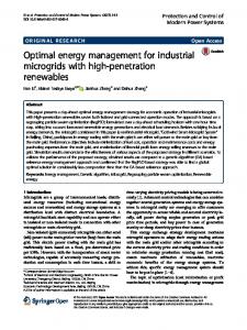
Figure 1. Centrally controlled LAN/PAN topology with uplink and downlink communication

Our focus is on point-to-multipoint wireless networks where all users are within the same collision domain with an access point (AP) to arbitrate exclusive channel (Fig. 1). We present a Methodology for Energy-Efficient Resource Allocation (MEERA) based on systems that can sleep and scale. To achieve this, a combination of each approach is leveraged to minimize energy consumption depending on the current channel conditions and amount of data to be delivered before the deadline for each user. Our solution exploits control knobs or control dimensions from (a) real radio frequency integrated circuit (RFIC) system models, (b) communication theoretic trade-offs and (c) link-layer scheduling. The system’s configuration is adapted to the current conditions by setting system control dimensions or knobs such as the transmission power, modulation and code rate. To evaluate MEERA, we exploit the energy-performance tradeoff by considering additional control dimensions such as the power amplifier (PA) back-off, a sleep-aware Medium Access Controller (MAC) protocol and packet retransmissions. We finally simulate the performance of MEERA using a realistic HIPERLAN/2 indoor channel model [9], with full-length MPEG-4 [10] encoded movies transmitted over a modified 802.11 MAC protocol [30]. A. Related Work For the past decade, there have been several initiatives to design energy-efficient processors [11, 12] primarily employing dynamic voltage scaling and low-power VLSI implementations. These methods, however, do not extend well for wireless transceivers, as the performance of analog circuits, which dominate the energy consumption, does not scale as monotonically with lower voltages as digital circuits. In addition, wireless communications present non-linear and discrete energy-performance tradeoffs between different modulation constellations, coding and transmit power [13], between modulation and active circuit energy consumption [14] and between transmission rates and shutting off the system [15]. To address this, researchers have approached the problem either from an information-theoretic perspective [14, 16] or from an implementation-specific viewpoint [11, 17]. In [14], modulation strategies for MQAM and MFSK are derived for delay-bound traffic. It is shown that when the transmit power and energy consumed by the circuitry are comparable (for short-range communication < 10m), the transmission energy decreases with the product of the bandwidth and transmit duration. They however only consider an idealized network

restricted to a single flow with no medium access controller (MAC) or link layer retransmissions, and with ideal continuous constellation sizes. In [16], the goal of scalable energy is framed as a convex optimization problem where multiple users lower their transmission rate to minimize energy consumption during transmission. They do not consider the fixed circuit energy consumed during idle and receive intervals. On the other hand, [13] explores the trade-off between transmission power control and physical layer (PHY) rate for a centrally controlled MAC with retransmissions. Their solutions are specific and applicable to the 802.11a PHY [1]. They derive bit-error rates based on simple AWGN channel models. They also consider only a single flow with no delay constraints or system sleep modes. A more general framework to exploit the energy scalability of transceivers is derived in [15]. They derive the operating regions when a transceiver may sleep or use transmission scaling for time-invariant and time-varying channels. The analysis is based on simplified physical layer energy models and only point-to-point file transfer traffic is considered. Approaches to trade-off energy and rate performance, taking into account implementation-specific aspects and real operating conditions are proposed in [11, 17]. An energyperformance trade-off is presented for a single user pair at design-time and depends on the system implementation. Offline energy optimizations for energy-scalable systems are proposed in [14, 15, 17]. They express the need for a practical runtime scheme to determine the configurations for one or more users. In order to derive optimal or near-optimal operating points, a framework is needed to consider the impact of the various control dimensions, the trade-offs between them and the overall benefit to the user. In [18], the authors present a useful approach to maximize the utility for multimedia applications given multiple resources and along multiple control dimensions. Our approach to minimize energy consumption has a similar basis, incorporating communications constraints and extended for use in dynamic wireless systems. MEERA first derives the optimal operating points in terms of transmission control and sleep durations at design time for a range of scenarios. At runtime, a lightweight scheme employs the best configurations for each flow’s channel state and application timeliness requirement over a MAC protocol. B. Organization of the Paper In the following section, we provide a formal framework for the generalized MEERA energy management technique. Section 3 applies the methodology to a system based on real RFIC and channel models and derives its energy-performance trade-off. In Section 4, we present simulation results for multiple users with delay-constrained traffic. Section 5 presents the concluding remarks.

II ENERGY-EFFICIENT DESIGN METHODOLOGY The design of low-power wireless systems needs to encompass RF components, adaptive physical layer algorithms, and the MAC protocol. In order to extract significant energy savings from the system, implementations and algorithms in the three layers must work harmoniously. Therefore, the

impact of each local control algorithm should be known on the total system energy consumption and user-related performance. This requires a sound methodology that can scale with the combinatorial explosion of the number of possible configurations and with the non-linear and implementation specific interaction of a system-dependent set of control dimensions. The following three observations show the need to integrate the energy-efficient approaches across layers. First, state-of-the-art wireless systems such as 802.11a devices are built to function at a fixed set of operating points and assume the worst-case conditions at all times. Irrespective of the link utilization, the highest feasible PHY rate is always used and the power amplifier operates at the maximum transmit power [8]. Indeed, when using non-scalable transceivers, this highest feasible rate results in the smallest duty cycle for the power amplifier. Compared to scalable systems, this results in excessive energy consumption for average channel conditions and average link utilizations. Recent energy-efficient wireless system designs focus on energy-efficient VLSI implementations and adaptive physical layer algorithms where a lower modulation rate requires a lower code rate and transmission power while maintaining the same receive SNR. For these schemes to be practical, they need to be aware of the hardware components’ energy efficiency at various operating points. Second, to realize sizable energy savings, systems need to shutdown the components when inactive. This is achieved only by tightly coupling the MAC to communicate traffic requirements of each user for scheduling shutdown intervals. Finally, there exist intricate tradeoffs between the adaptive physical layer schemes and satisfying the requirements of multiple users. As all users share a common channel, lowering the rate of one user reduces the available time for the second delay-sensitive user. This forces the second user to increase its rate, consume more energy and potentially suffer from a higher bit error rate. Our methodology for energy-efficient resource allocation, MEERA, therefore needs to address ways to couple these three layers to find the optimal setting of the control dimensions and provide for a provable efficient scheme to manage system-wide power management dimensions at runtime. First, we formally state the MEERA Resource Management model, focusing on the system design goals and general definition of the control dimensions. Next, we formally state the run-time resource allocation problem. Finally, we show how we can transform the control dimensions into a very efficient form to be handled at runtime. In essence, our goal is to present a general and flexible platform-independent cost (e.g. energy) optimization followed by a mapping to a practical wireless context based on actual system models to minimize energy consumption. A. MEERA Resource Management Model Consider a wireless network as in Fig. 1 where multiple nodes are controlled centrally by an access point (AP). Each node (such as a handheld video camera) desires to transmit or receive frames at real-time and it is the AP’s responsibility to assign channel access grants. The resource allocation scheme within the AP specifies each user’s system configuration

settings for the next transmission based on the feedback from the current transmission. It must ensure that the nodes meet their performance constraints by delivering their data in a timely manner while consuming minimal energy. The problem is stated formally as: 1) MEERA Definitions The network consists of n flows {F1, F2, …, Fn} with periodic delay-sensitive frames or jobs. For notational simplicity, we assume a one-to-one mapping of flows to nodes, but our design methodology is applicable to one or more flows per node. Each flow i, 1 ≤ i ≤ n, is described by the following properties: (a) Cost Function (Ci): This is the optimization objective, e.g. to minimize the total energy consumption of all users in terms of Joules/Job. In, for example, a video context, a job is the timely delivery of the current frame of the video application. (b) QoS Constraint (Qi): The optimization has to be carried out taking into account a minimum performance or QoS requirement in order to satisfy the user. As delivery of realtime traffic is of interest (e.g. video streaming), we describe the QoS in terms of the job failure rate (JFR) or deadline miss rate [19]. JFR is defined as the ratio of the number of frames not successfully delivered before their deadline to the total number of frames issued by the application over the lifetime of the flow. The QoS constraint is specified by the user as a targetJFR (i.e. JFR*), to be maintained over the lifetime of the flow. (c) Shared Resource (Ri,l), 1 ≤ i ≤ n, 1 ≤ l ≤ r: Multiple resource dimensions, r, could be used to schedule flows or tasks in the network, e.g. time, frequency or space. In this paper, we consider the restricted case where access to the channel is only divided in time. Therefore, time, is the single shared resource (i.e. r = 1) and the total available quantity is denoted by R. The fraction of resource consumed by the ith node is denoted by Ri. The maximum time available for any flow is Rimax, which is the frame period for periodic traffic. (d) Control Dimensions (Ki,j), 1 ≤ i ≤ n, 1 ≤ j ≤ k: For a given wireless LAN architecture, there are k platform independent control knobs or dimensions, such as modulation, code rate, PA output power, etc. that control the received SNR related to the resource utilization in terms of the transmission time per bit, given the current path loss. In our case study presented in section III, we identify additional control dimensions such as the PA back-off which presents a tradeoff between the amplifier linearity and efficiency. The control dimension settings are discrete, inter-dependent and together have a nonlinear influence on the cost-function. We define a setting of all k knobs for node i to be the configuration point K i , j .We will define a relationship between K i , j to Qi, Ci and Ri in the next section. (e) System state (Si,m), 1 ≤ i ≤ n, 1 ≤ m ≤ s: As we are operating in a very dynamic environment, the system behavior will vary over time. There are s environmental factors independent of the user or system’s control that are represented by the system state variable, Si,m. Both the system cost-function and resources required depend on the system state. In a wireless environment

with say VBR video traffic, the system state is determined by the current channel state and the current application frame size. The scheduling algorithm within the AP is executed with a period based on the channel epoch and the rate at which the data requirements change. To summarize, each flow Fi is associated with a set of possible system states Si,m, which determines the mapping of the control dimensions K i , j to the cost ( K i , j ÆCi(Si,m)) and resource ( K i , j ÆRi(Si,m)). It is essential to note that for each user, depending on its current state, the relative energy gains possible by rate scaling and sleeping are different and should hence be exploited differently. Each user experiences different channel and application dynamics, resulting in different system states over time, which may or may not be correlated with other users. This is a very important characteristic which makes it possible to exploit multi-user diversity for energy efficiency. 2) MEERA Model Properties The key aspects of MEERA are the mapping of the control dimensions to cost and resource profiles respectively, and the generality of this mapping. A resource (cost) profile describes a list of potential resource (cost) allocation schemes needed for each configuration point K i , j . A more case-specific mapping is provided in Section III. These profiles are then combined, as shown in Fig. 2, to give a Cost-Resource trade-off function, which is essential for solving the resource allocation problem. A Cost-Resource trade-off function represents the behavior of the system for one user in a given state. Cost profile properties • Every flow has a known minimum and maximum cost (e.g. Joules/job) over all control dimensions, which is a function of the desired JFR* and the system state (e.g. channel state). The cost range (difference between maximum and minimum) needs to be determined once by measuring the impact of each control dimension on the energy consumption over all system states. For example, a flow requiring high channel utilization, due to a high application data rate or a channel with a large packet error rate (PER), would conserve energy primarily by scaling transmission rate and power than from shutdown. • The discrete configuration settings for each control dimension can be ordered according to their increasing Cost. • The overall system cost, C, is defined as the weighted sum of costs of all flows, where each flow can be assigned a certain weight depending on its relative importance or to improve fairness [19] (e.g. higher weight for flows with higher average data rate). C =

n

∑w C i =1

i

i

Resource profile properties • Every flow has a known minimum and maximum resource requirement (e.g. allocated frame transmission time) across all control dimensions. This is a function of the desired JFR*

and system state and is calculated from the system model (detailed in section III). • Depending on the current system constraints and possible configurations, each flow has a minimum resource requirement Rimin. We assume the minimum resource requirements can be satisfied for all flows under worst-case load and channel conditions. Hence, no overload occurs and all flows can be scheduled. However, in the delivery of nonscalable video applications under worst-case conditions, a system overload may occur and one or more flows will need to be dropped. While the policy to drop flows is out of the scope of our optimization criterion, a practical system may employ policing that is fair to the users as in [19]. • The per-dimension discrete control settings can be ordered according to their minimal associated Resource requirement. • The overall system resource requirement, R, is defined as the sum of the per flow requirements: R=

n

∑R i =1

i

B. MEERA Resource Allocation Problem We recall that our goal is to assign transmission grants via the AP, resulting from an optimal setting of the control dimensions to each node such that the per-flow QoS constraints for multiple users are met with minimal energy consumption. For a given set of resources, control dimensions and QoS constraints, the scheduling objective is formally stated as: n

min ∑ wi C i ( S i ,m ),m = 1,..., s C

i =1

subject to: JFR i ≤ JFR i* , i = 1,..., n n

∑R i =1

i ,l

≤ Rl

max

, l = 1,..., r

(QoS Constraints) (Resource Constraints)

K i , j → Ri ,l ( S i ,m ), j = 1,..., k ; m = 1,..., s (Resource Profiles)

K i , j → Ci ( S i ,m )

(Cost Profiles)

The solution of the optimization problem yields a set of feasible operating points, {Ki,j}, which fulfill the QoS target, maintains the shared resource constraint and minimizes the system cost. In order to determine this configuration K, we next propose a two-phase solution approach. C. Two-phase Solution Approach When considering energy-scalable systems, the number of control dimensions is large (even on the order of 106) and leads to a combinatorial explosion of the possible system configurations. Hence, a pragmatic scheme is needed to select the configurations at runtime. We achieve this by first determining the optimal configurations of all control dimensions at design or calibration time. At runtime, based on the channel condition and application load, the best operating point is selected from a significantly reduced set of possibilities.

Costi

Resourcei

Costi

Costi

Pi

K1

Kj

K1

Kj

Convex Minorant Resourcei

Resourcei

Figure 2. At design time, a Cost and Resource profile is determined for each set of control dimensions. This mapping depends on the current state of each node. The minimum Cost-Resource tradeoff is derived from this mapping to give operating points used at runtime.

1) Design-Time Phase A property of our model is that the control dimensions can be ordered according to their minimal cost and resource consumption, describing a range of possible costs and resources for the system. For each additional unit of resource allocated, we only need to consider the configuration that achieves the minimal cost for that unit of the resource. For each possible system state (e.g. for different channel and application loads), the optimal operating points are determined by pruning the Cost-Resource curves to yield only the minimum cost configurations, which will be denoted by Ci(Ri), at each resource allocation point. We define a function pi : R → C , such that p i ( Ri ( S i , m )) = min{C i ( S i ,m ) | ( K i → Ri ( S i , m )) ∧ ( K i → Ci ( S i , m ))}

which defines a mapping between the Resource and the Cost of a certain configuration, k, for a node in a state, Si, as shown in Fig. 2. Considering the resulting points in the Cost-Resource space, we are only interested in the ones that represent the optimal trade-off between the energy and resource needs for our system. Indeed, the trade-off between transmission time and transmission energy is convex - a fundamental property for wireless communication bounded by Shannon’s channel capacity [20]. Although the discrete settings and non-linear interactions in real systems lead to a deviation from this optimal trade-off, it can be well approximated as follows. We calculate the convex minorant [21] (i.e. most energyefficient points along both the Cost-Control dimensions and the Resource-Control dimension curves) of these pruned curves along the Cost and Resource dimensions, and consider the intersection of the result. As a result, the number of operating points is reduced significantly (Fig. 3). We briefly consider the tradeoffs present in our system: increasing the modulation constellation size decreases the transmission time but results in a higher PER for the same channel conditions and PA settings. The energy savings due to decreased transmission time must offset the increased expected cost of re-transmissions. Also, increasing the transmit power increases the signal distortion due to the PA nonlinearity [26]. On the other hand, decreasing the transmission power also decreases the efficiency of the PA. Similarly, it is not straightforward when using a higher coding gain, if the decreased SNR requirement or increased transmission time dominates the energy consumption. Considering the tradeoff between sleeping and scaling, a longer transmission at a lower and more robust modulation rate needs to compensate for the opportunity cost of not sleeping earlier. Finally, as all users

share a common channel, lowering the rate of one user reduces the available time for other delay-sensitive users. This compels one or more of the other users to increase their rate, consume more energy and potentially suffer from a higher bit error rate. At design time, we derive the convex minorant of the Cost (energy consumption) and Resource (time) of the transceiver for one user across all system states. 2) Run-Time Phase As the system state of all the users is only known at runtime, a light-weight scheme is necessary to assign the best system configurations for each user. We employ a greedy algorithm to determine the per-flow resource usage, Ri, for each application to minimize the total system cost, C. The algorithm traverses all flows’ Cost-Resource curves and at every step consumes resources corresponding to the maximum negative slope across all flows. This ensures that for every additional unit of resources consumed, the additional cost saving is the maximum across all flows [21]. We assume that the current channel state and application demand are known for each node. If this changes, the allocation can be recomputed. This information is obtained by coupling the MAC protocol with the resource manager and is explained in the next section. We determine the optimal additional allocation to each flow, Ri > 0,1 ≤ i ≤ n , subject to

∑

n i =1

R i ≤ R . Our greedy algorithm is based on Kuhn-

Tucker [21]: a. Allocate to each flow the smallest resource possible for the given state, Rmin. By assumption, all flows are schedulable under worst-case conditions, i.e. ∑n R min ≤ R . i =1

b. Let the current normalized allocation of the resource to flow, Fi, be Ri, 1 ≤ i ≤ n. Let the unallocated quantity of the available resource be Ravl. c. Identify the flow with the maximum negative slope, |Ci’(Ri)| – representing the maximum decrease in cost per resource unit (i.e. moving right and downward the Ci ( Ri ) convex minorant in Fig. 3). If there is more than one, pick one randomly. If the value of the minimum slope is 0, then stop. No further allocation will decrease the system cost further. d. Increase Ri by the amount till the slope changes for the ith flow. Decrement Ravl by the additional allocated resource and increment the cost C by the consequent additional cost. Return to step b until all resources have been optimally allocated or when Ravl is 0. In our implementation, we sort the configuration points at design-time in the decreasing order of the negative slope

between two adjacent points. The complexity of the runtime algorithm is O(L.n.log(n)) for n nodes and L configuration points per curve. In Section III, we demonstrate that for a practical system in each possible system state (i.e. channel and frame size), the number of configuration points to be considered at runtime is relatively small (~20). Taking into account that the relation Ci(Ri) derived at design time is a convex trade-off curve, we now prove that the greedy algorithm leads to the optimal solution for continuous resource allocation. Following that, we extend the proof for real systems with discrete working points to show that the solution is within bounded deviation from the optimal. Theorem 1 For a continuous resource allocation to be optimal, a necessary condition is ∀ i, 1 ≤ i ≤ n, Ri = 0 or for any flows {i, j} with Ri > 0 and Rj > 0, the cost slopes Ci`(Rj) = Cj`(Rj). Proof: For a continuous differentiable function, the KuhnTucker [21] theorem proves such a greedy scheme is optimal. Suppose for some i ∫ j, let the optimal resources allocation be Ri > 0, Rj > 0, and |Ci’(Ri)| > |Cj’(Rj)|. As the savings in cost per unit resource for Fi is larger, we can subtract an infinitesimal amount of resource r from Fj and add it to Fi. The total system cost is reduced and this contradicts the optimality assumption. For a real system, however, the settings for different control dimensions such as modulation or transmit power are in discrete units. This results in a deviation, ∆, from the optimal resource assignment. We now show that the worst-case deviation from the optimal strategy is bounded and small. Theorem 2. ∃ 0 ≤ ∆ < ∞ , such that COPT ≤ C MEERA ≤ COPT + ∆ , where COPT is the optimal cost (energy consumed by all users) in the continuous case and CMEERA is the cost in the discrete case. Proof: For each flow, {F1, F2, …, Fn}, the aggregate system resources consumed are stored in the decreasing order of their negative slope across all per-flow Cost-Resource Ci(Ri) curves. Based on this ordering, the aggregate system C(R) trade-off is constructed, consisting of segments resulting from individual flows. The greedy algorithm traverses segments of the aggregate system C(R) curve, consisting of successive additional resource consumptions for a unit of data (at maximum cost decrease), until the first segment, s, is found that requires more resource than the residual resource capacity Ravl to realize the extra cost saving at the end of the segment (Fig. 3). Let the two end points of the final segment s be (rs, cs) and (rs+1, cs+1) in C(R). Let (rc, cc) be the optimal resource allocation in the optimal combined Cost-Resource curve.

COPT ≥ CMEERA - (rc – rs) (cs+1 – cs)/( rs+1 – rs) > CMEERA - (rs+1 – rs) (cs+1 – cs)/( rs+1 – rs) = CMEERA - (cs+1 - cs) We observe that cs - cs+1 ≤ ∆, therefore CMEERA - COPT < ∆. Moreover, we note that with more dimensions (Ki,r) considered, a better approximation can be obtained.

Cost

(rs, cs) s

(rc, cc) (rs+1, cs+1)

Resource Rl Figure 3. Bounded deviation from the optimal in discrete Cost-Resource curves

III. SYSTEM OVERVIEW We now illustrate application of MEERA mapped to a specific wireless system with periodic and delay-sensitive video traffic (Fig. 4). We first model a scalable broadband transceiver from actual RF components and define its control dimensions. The different environmental dynamics such as the channel condition and current application demand are then categorized into channel states and packet sizes. Following this, the influence of the control dimensions to both cost and resource is mapped at design-time, taking into account the QoS requirements and system constraints. Finally, we show how at runtime, MEERA uses the feedback information of the channel state and application demand to select the optimal operating point for each node and how this can be embedded in existing access schemes.

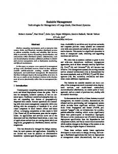
A. Energy-Performance Control Dimensions For a broadband transceiver, we identify several control dimensions that tradeoff performance for energy savings and vice versa. Our system modeling is based on an 802.11a [1] direct conversion transceiver implementation with turbo coding [24] (Fig. 5). Four control dimensions have a significant impact on energy and performance for these OFDM transceivers: the modulation order (NMod), the code rate (Bc), the power amplifier transmit power (PTX) and its linearity specified by the back-off (b). We focus on the power amplifier (PA) control knob as PA’s generally are the most power-hungry component in the transmitter consuming upwards of 600mW [25]. The major drawback for 802.11a OFDM modulation is the large 17dB peak-to-average ratio (PAR) of the transmitted signal. A high PAR renders the implementation costly and inefficient since efficient PA designs require a reduced signal dynamic range [26]. However, reducing the PA’s dynamic range clips the transmitted signal and increases the signal distortion. A back-off, b, from the peak signal amplitude or saturation power, can be used to steer the linearity of the system versus the energy efficiency of the PA [17]. The back-off is defined as the ratio of the average PA output power to the output power corresponding to the 1dB gain compression point (Fig. 6). The saturation power and signal distortion for class A amplifiers (used with OFDM) are controlled by modifying the bias current of the amplifier, and directly influences its energy consumption.

A. Control Dimensions

B. Map for System Dynamics

- Constellation - Code Rate - PA Output Power - PA back-off

- Traffic - Channel S2

C. Map for System Constraints

- Target Job Failure Rate - Access Protocol: Central Controlled Reliable (ACK-overhead) Time-schedule based Cost

S1

D. Run-time Management - Exploit C(R) to schedule flows C

R

Resource

802.11e HCF Poll-TxOp-Ack

Figure 4. Design Methodology flow for energy management in dynamic systems.

Hence, we save energy from the increased PA efficiency, provided we ensure that the received signal to noise and distortion ratio (SINAD) is above the required sensitivity and do not need to retransmit the packet. For the system to be practical only discrete settings of the control dimensions are considered (listed in Table 2). We consider the eight PHY rates supported by 802.11a based on four modulation and three code rates (Table 2). The bit rate (Bbit) achieved for each modulation-coding pair with Nc OFDM carriers, NMod bits per symbol and Symbol rate B is given by: (1) Bbit = N c × N Mod × Bc × B Based on the bit rate, communication performance is determined by the bit error rate (BER) at the receiver. When transmitter non-linearity is considered, the BER is expressed as a function of the SINAD. The SINAD is written as a function as the power amplifier back-off, given output power PTx and channel attenuation A as: PTx × A (2) SINAD = A × Di (b) + kT × W × NF PTx PPA = η PA (b)

(3)

where the constants k, T, W and NF are the Boltzman constant, working temperature, channel bandwidth and noise figure of the receiver respectively. The relation between the power amplifier back-off b and the distortion has been characterized empirically for the Microsemi LX5506 [28] 802.11a PA in Fig 6. The PA power (PPA) can be expressed as the ratio of the transmit power (PTx) to the PA efficiency (ηPA) that is related to b by an empirical law fitted on measurements (3). We assume the energy consumption of the digital baseband is a linear function of time and block size for the turbo decoding at the receiver [24]. The block size used for the turbo coding is 288 bits. Based on current implementations [25], the frequency synthesizer, ADC, DAC, LNA and filters are

assumed to have a fixed front-end power consumption PFE as given in Table 2. The time needed to wake-up the system (stabilization time for the PLL in the frequency synthesizer) is assumed to be 100 µs, which is optimistic but can be achieved when designing frequency generators for this purpose. Application layer frames are fragmented at the link layer. We obtain the following expressions for the energy needed to send or receive a fragment of length Lfrag, as a function of the current knob settings: E Tx = (

T T PPA + PFE + PBB ) × L frag Bbit

E Rx = (

R PFE + PBBR R + E DSP ) × L frag Bbit

(5)

where PTBB and PTDSP are the base-band and digital signal processor’s power consumption.

B. System State To determine the Job Failure Rate and total expected energy consumption, the system dynamics must be considered. For this case study, the channel and the traffic are considered to vary independently in discrete states. 1) Traffic Model Both constant bit rate (CBR) and variable bit rate (VBR) traffic are studied. VBR traffic consists of MPEG-4 flows. A Transform Expand Sample-based MPEG-4 traffic generator [29] that generates traffic with the same first and second order statistics as an original MPEG-4 trace is used. MPEG-4 traffic is extremely bursty with the peak-to-average frame size ranging from 3 to 20. All fragmentation is done at the link layer and if a frame is not completely delivered to the receiver by its deadline, it is dropped. All applications employ UDP over IP. Performance

Energy Model

MAC Model

Control Dimensions

PTFE = 200mW

Lfrag = 1024B

Back-off (dB) {6 to 16}

= 200mW

TACK = 52ms

Nc = 48

PTDSP = 50mW

TPLCP = 20ms

T = 198K Nf = 10dB

PRDSP = 50mW ERDSP = 8.7nJ/b

Block = 288

Pout (dBm) {0 to 20} Modulation {BPSK, QPSK, 16-QAM, 64QAM} Code Rate {1/2, 2/3, ¾} JFR* = 10e-03

Model W = 20MHz B = 250Kbaud

Figure 5. 802.11a OFDM Direct Conversion Transceiver

(4)

R

P

FE

TSIFS = 16ms

DC power in mW (class A)

S1 200

PA energy consumption in mode 3

150 100 50

S5 PA energy comsumption in mode 2 PA energy consumption in mode 1

0 −20

−15

−10

−5

0

S4 5

10

15

20

25

30

S3 S1

20 actual output power in dBm

S2

S4

PA mode 3 10

S3

S2

PA mode 2

S5

PA mode 1

0 −10 −20 −30 −20

−15

−10

−5

0 5 10 15 expected (linear) output power in dBm

20

25

Fig. 6 Power amplifier with variable bias

Each frame size maps to a different system state. A frame size is determined in a number of MAC layer fragments, which is assumed to be 1024 bytes long for this experiment. From our results, we observe that for a given frame size, extrapolating the results for a curve within five fragments results in a very low approximation error. As the maximum frame size is assumed to be within the practical limit of 50 fragments long, we only construct Cost-Resource curves for 1, 2, 3, 4, 5, 10, 20, 30, 40, 50 fragments per frame. 2) Channel Model We use a frequency selective and time varying channel model to compute the PER for all transceiver settings. An indoor channel model based on HIPERLAN/2 [9] was used for a terminal moving uniformly at speeds between 0 to 5.2 km/h (walking speed). Experiments for indoor environments [27] have found the Doppler spread to be approximately 6Hz at 5.25GHz center frequency and 3Hz at the 2.4GHz center frequency. This corresponds to a coherence time of ~166ms for 802.11a networks. A set of 1000 time-varying frequency channel response realizations (sampled every 2ms over one minute) were generated and normalized in power. Data was encoded using a turbo coder model [24] and the bit stream was modulated using 802.11a OFDM specifications. For a given back-off and transmit power, the SINAD at the receiver antenna was computed by equation (2). We assume a path-loss of 80dB at a distance of 10m. The signal was then equalized (zero-forcing scheme), demodulated and decoded. From the channel realization database, a one-to-one mapping of SINAD to receive block error rate was determined for each modulation and code rate. The channel was then classified into 5 classes, determined by a 2dB difference at turbo code block error rate (BlER) 10e-3 (Fig. 7(a)). We use a similar 2dB discrete step for the PA profile (Fig. 6). In order to derive a time-varying link-layer error model, we associate each channel class to a Markov state, each with a probability of occurrence based on the channel realizations database (Fig. 7(b)). Given this five-state error model, we are able at runtime, to efficiently model the PER for different configurations. The PER is obtained in equation (6) by assuming the block errors follow a binomial process for a packet size of Lfrag bits and a block size of 288 bits: L / 288 (6) PER = [1 − (1 − BlER) ] frag

Figure 7(a) Performance across different channel states. (b) Channel states histogram

30

C. Cost and Resource Profile Mapping In the previous sections we determined, for each system state, expressions for the energy to send (4) or receive (5) a fragment, and the PER experienced by this fragment (6), based on the system configuration setting. From these expressions and the system state, we now derive the exact mapping of the set of control dimensions K to the cost and resource dimensions. This mapping should take into account the protocol and system constraints, and the QoS requirements. For the protocol constraints, the IEEE 802.11e MAC scheme [30] is considered as it is an emerging standard for QoS support (Fig. 8). From [19], we observe that the contention-free burst or transmit opportunity (TXOP) grant of 802.11e Hybrid Coordination Function (HCF) can significantly improve the network QoS. A TXOP is defined as an interval of time when a user has exclusive channel access and is defined by a start time and a maximum duration. All TXOPs are contention free and are assigned by the AP. The shared resource is time, and therefore the resource allocation problem is to determine the optimal TXOP for each flow. We now incorporate the protocol overhead and timing into the resource consumption. Let EACK and TACK be the energy and time needed to receive an ACK packet. EHeader and THeader are the energy and time for the MAC and PHY headers. The energy and time needed for a successful and failed1 frame transmission is then be determined using parameters based on 802.11e, listed in Table 2: (7) E good ( K ) = E K + E Header + ( 2 × Tsifs × PIdle ) + E ACK E bad ( K ) = E K + E Header + ((Tsifs + T ACK ) × PIdle )

(8)

T good ( K ) = TK + THeader + ( 2 × Tsifs ) + T ACK

(9)

Tbad ( K ) = T good ( K ) − T sifs

(10)

The QoS metric of interest is the target Job Failure Rate (JFR*). A job is the delivery of an application layer frame. A job failure occurs when the entire frame is not delivered by its deadline. We assume the deadline is equal to the flow period. For successful transmission of a frame, we adopt the policy that each fragment of a frame should be transmitted or retransmitted using the same configuration K i , j , which we will 1

For a failed transmission, we wait the propagation time, SIFS time and the time normally needed to receive (decode) the ACK. Only after that time we can be sure the ACK is not received and the packet transmission has failed.

Ttot_good 1 frag

Start TXOP SIFS

Uplink Downlink

Frag. 1

SIFS

HCF Poll

Frag. 2

Ttot_bad 1 frag

Start TXOP SIFS

Uplink Downlink

SIFS ACK

Frag. 1

SIFS

HCF Poll

Frag. 1 ACK

Figure 8. Timing of successful and failed uplink frame transmission with 802.11e HCF.

denote by K for notational simplicity. This is a good approximation to the optimal transmission approach which adapts the control dimensions depending on the outcome of the previous fragment’s transmission (conditional recursion which is complex to solve at runtime). For the approximation, we derive a recursive formulation to compute the expected energy EK, the timeslot needed TXOPK, and the expected failure rate JFRK, for each system state determined by the frame size of m fragments and channel state. For notational simplicity, we will also omit the channel state index. Each packet is transmitted with configuration K, for which we can determine the PERK, based on equation (6). The probability that the frame is delivered successfully with exactly (m + n) transmissions (including n retransmissions), is given by the recursion: min( m , n ) (11) S m (K ) = C m × ( PER ) i × (1 − PER ) m −i × S i ( K )

∑

n

i =1

i

K

n −i

K

(12)

S 0m ( K ) = (1 − PERK ) m

in which C denotes the number of possibilities to select i fragments out of m. Hence, the probability to deliver the frame consisting of m fragments correctly with maximum n retransmissions is n (13) 1 − JFR m ( K ) = S m ( K ) m i

∑

n

j =0

j

Figure 9. The mapping for the PA output power & back-off control dimension for a fixed setting of the modulation & code rate control dimensions

E nm ( K ) = E nm ( K ) + JFR nm ( K ) × [ E bad ( K ) + m

∑S j =1

j n

( K ) × (( j × E good ( K )) + ( n × E bad ( K )))]

As a result, we determine the E, TXOP, and JFR as a function of frame size, channel state and number of retransmissions for each configuration K. This specifies the full cost and resource profile for the system, taking into account the protocol constraints. In Fig. 9, the impact of the PA control knobs (PA back-off and PA transmit power) on the resource (TXOP) and cost (energy) is illustrated.

Therefore, the failure to deliver an entire application layer frame before the deadline is marked as a job failure. As control frames are much shorter and less susceptible to errors, we assume they do not suffer packet errors. The time needed to send m fragments with maximum n retransmissions, for configuration K, is then: (14) TXOPnm ( K ) = [ m × Tgood ( K )] + [ n × Tbad ( K )] The average energy needed to transmit m fragments, with maximum n retransmissions, and configuration K considers the expected energy of retransmissions for the given configuration: n (15) E m ( K ) = S m ( K ) × ((m ×E ( K )) + ( j × E ( K ))) n

∑ j =0

n

good

(16)

bad

The expected energy for a given configuration is the sum of the probabilities that the transmission will succeed after m good and j bad transmissions multiplied by the energy needed for good and bad transmissions. In order to have the correct expected energy consumption, a second term should be added to denote the energy consumption for a failed job, hence when there are less than m good transmissions, and (n+1) bad ones: Figure 10.(a) Ci(Ri) curve for different channel states (CS), (b) Ci (Ri) curves for different frame sizes

P1

P2

P3

P4

P3

P2 P1

Packet Arrival

P4

P1 P1

30ms fram e period

Scheduler B uffer C ontents [buff 1, buff 2]

P3

P2 P2

P3

Sleep between service

C hannel Activity Packet Transm itted Sleep Activity Tim e

Figure 11. MAC with two-frame buffering to remove data dependencies and maximize sleep durations. By the third period of the single flow shown, frames 1 and 2 are buffered and frame 1 begins service. As the transmission duration of frame 2 is known at this time, the sleep duration between completion of frame 1 until the start of service of frame 2 is appended in the MAC header

Only the mapping that corresponds to the smallest TXOP and Energy consumption for given constraints is plotted. Fig. 10 shows the merged and pruned Energy-TXOP curves for (a) different channel states and (b) different frame sizes. We can see that the total range in energy consumption is large, both within and across system states. The large tradeoff proves our conjecture that traditional systems designed for a fixed and worst- cast scenario, result in significant energy wastage.

frame period (e.g. 30 ms for high-quality video) of the flow in the system with the highest frame rate. We assume the channel is slow fading such that the channel state used to make the scheduling decision is still valid during the servicing of the TXOP. In [27], channel measurements show coherence times of up to 166ms for stationary objects and moving scatterers.

D. Link Layer Resource Management Based on the Energy and TXOP curves for each node, the scheduler in the AP can derive a near-optimal resource allocation at run-time using the greedy scheme described in Section II. The scheduler requires feedback on the current state of each user and then communicates the TXOP and transmission configuration decisions to the users. The MAC is responsible for resource allocation of the shared channel. The packet-scheduling algorithm in the AP decides which node is to transmit, when, and for how long. In order to instruct a node to sleep for a particular duration, the AP needs to know when the next packet will be scheduled. Waking a node earlier than the schedule instance will waste energy in the idle state. Waking the node later than the schedule instance, will cause it to miss the packet’s deadline or waste system resources by transmitting at a higher rate. Our sleep-aware MAC protocol therefore buffers two frames to eliminate data dependency due to the application and channel. Buffering just two frames informs the AP of the current traffic demand but also the demand in the next scheduling instance. As shown in Fig. 11, the AP now needs to communicate with each node only at scheduling instances. As the real-time stream’s packets are periodic, we eliminate all idle time between transmission instances. The scheduler ensures in every frame period all flows are scheduled to meet their deadlines, each with the best TXOP to minimize overall energy consumption. This is accomplished by adding just three bytes in the MAC header for the current channel state and the two buffered frame sizes. Protocols such as 802.11e [30] provide support for queue sizes and therefore require only minor modifications. In every transmission to the AP, each node communicates its channel state and packet sizes of the two head of the line packets. In the ACK, the AP instructs the node to sleep until the time of the next scheduling instance and also assigns it the duration of its next TXOP. The scheduling decision is hence be made every

Based on the MEERA methodology and the transceiver system model, we would like to verify the energy savings over a range of practical scenarios. For all results presented here, the target JFR* is set to 10e-3 which is a reasonable value for wireless links. The focus is on real-time streaming media applications to show the Energy-Performance tradeoff. To keep the system simple, we are not application-aware and do not differentiate frames based on frame type. In order to evaluate the relative performance of MEERA, we consider four comparative transmission strategies: 1. MEERA: This is the optimal operating scheme considering the energy tradeoff between sleep and scaling, exploiting multi-user diversity. The operating point is determined from the Ci(Ri) curves derived in Section III, and the runtime algorithm described in section II. C. 2. MEERA-no sleep: This scheme uses the Ci(Ri) curves to determine the optimal TXOP when no sleeping is supported. The same runtime algorithm is used and the nodes remain in the idle state after completion. The purpose of this case is to show the contribution of sleeping. 3. Fixed: The transceiver uses the PA back-off and output power at the highest setting with the highest feasible modulation and code rate that will successfully deliver the packets. After successful transmission, it switches to sleep. This approach is proposed by commercial 802.11 interfaces [8], which only aim to maximize the sleep duration. 4. Fixed–no sleep: Similar to Fixed, the transceiver here remains in the idle mode after successful transmission. This is the base operating scheme of current wireless LAN transceivers with no power save features enabled. For each of these schemes, the Cost-Resource curves were determined and used by the scheduling scheme implemented in the Network Simulator ns-2. This simulator has been extended with transceiver energy and performance models, and a slow fading channel model. All results given below are based on the total energy consumed by a node to deliver its flow over a duration long enough to statistically capture the dynamics

IV. NUMERICAL RESULTS

present in the scenario. Our simulation model implements the essential functions of the 802.11e with beaconing, polling, TXOP assignment, uplink, and downlink frame exchange, fragmentation, frame retransmission and variable super-frame sizing. All nodes can hear and interfere with each other. A. Impact of the System State Consider the scenario where a single user has to deliver a fixed one-fragment frame each scheduling period. In Fig. 12(a), the relative energy consumption (normalized by the maximum energy consumed by Fixed over all cases), is plotted for the four schemes over different fixed channel states. As expected, MEERA outperforms the other techniques in each system state since it takes advantage of the energy that can be saved by both sleeping and TXOP scaling. The energy needed to transmit a unit of data increases from best to worst channel state due to a combination of (a) the lower modulation rate necessary to meet the higher SINAD requirement (hence smaller sleep duration), (b) a higher required output power to account for the worse channel and (c) the increased cost of retransmissions. We observe, for example, for the best channel state, the energy consumption is low for both the Fixed and MEERA approaches. The energy gains for this channel state primarily result from sleeping. On the other hand, for the worst channel state, the transmission energy becomes more dominant and TXOP scaling is more effective. We now look at the energy gains contributed by sleeping and scaling over a range of link utilizations by varying the frame size over a fixed channel state. For larger frame sizes, the TXOP scaling in MEERA-No sleep contributes significantly to the energy saving. This observation is illustrated in Fig. 12(b), where the relative gain for the different techniques – compared to the Fixed-no sleep case – are plotted over a series of frame sizes, for channel state 3.

22

Fixed - No Sleep Fixed MEERA - No Sleep MEERA

20 18 Total Energy Gain

B Impact of Link Utilization We now consider a multiple user scenario where the TXOP assignments are based on the user’s application data-rate requirement and the constraints enforced by other users sharing the same link. In this subsection, we present simulation results for CBR and MPEG-4 traffic over a static channel. We study the influence of the aggregate link utilization on the per-flow energy consumption for CBR flows over a static channel. The effective throughput of 802.11e, after considering protocol overheads for the first channel state, is approximately 30Mbps when the highest modulation constellation is used. In the experiment described by Fig 13(a), the link utilization is increased in steps of 2.1Mbps for CBR flows up to the maximum link capacity. We observe the per-flow energy consumption of MEERA increases as the aggregate system load increases. At higher loads due to a large number of flows, a smaller TXOP (with a higher rate and transmission power) from the Ci(Ri) curve is assigned to each flow resulting in higher per-flow energy consumption. The difference with MEERA-No sleep is most noticeable since the possibility to scale is reduced with increasing system load. For multiple users, it is always beneficial to enable sleeping as it is influenced to a lesser extent by the utilization of other flows. In Fig 13(b), we analyze the energy consumption for bursty MPEG-4 flows by increasing the number of simultaneous flows, each with an average rate of 2Mbps and peak-to-mean frame size ratio of ~3.5. It is important to note that as we do not force the system into overload, we consider only moderate link utilization (< 70% avg. load at the highest transmission rate). Job failures due to overload should be smaller than the target JFR*. MEERA consumes the least energy as it efficiently exploits scaling for the larger peak-to-average frame size ratio with sleeping.

16 14 12 10 8 6 4 2 0

5

10

20 30 Number of Fragments

40

50

Figure 12(a). Expected energy consumption across different channel states for 1 fragment. (b) Relative energy consumption by sleeping and scaling for different system loads in best channel state

Figure 13 (a). Energy consumption per flow as a function of the aggregate system load for CBR traffic (b) Energy consumption per flow as a function of mean per-flow data rate for MPEG traffic

Figure 14. Energy consumption for CBR traffic over a time-variant channel as function of aggregate system load

Compared to the CBR case, MEERA consumes more energy for the same average rate but MEERA-no sleep consumes lower energy showing that it is important for the energy management scheme to utilize rate scaling to leverage the multiplexing gain with bursty traffic.

C. Impact of Channel Dynamics We now consider a 5-user scenario to understand the impact of dynamic channel variations on energy consumption. The channel varies independently over all the users on a frame-byframe basis. In Fig 14, as the total system load is increased from 2.5 Mbps to 10 Mbps for five CBR flows, we make two observations: First, for the same system load, we see an increase in energy consumption when compared to the static channel in the best state. This is because during every scheduling cycle, the flows experiencing worse channel states require more transmission time (due to lower constellation) and therefore consume more energy. In addition, they force the other flows to transmit in a smaller TXOP and increase their energy consumption too. Second, the contributions to energy saving are almost evenly split between sleeping and scaling. This suggests that it is possible to do at least twice as better than schemes that just propose maximizing the sleep duration. The combination of sleep and scaling in MEERA delivers an overall system gain factor from 2 to 9 compared to Fixed (with sleep) and 2 to 5 compared to MEERA-no sleep (with scaling). V. CONCLUSION We propose a methodology for energy efficient resource allocation, MEERA, to minimize energy consumption of a wireless transceiver while meeting the timeliness requirements for multiple users. MEERA is a cross-layer optimization scheme that fully exploits the possible energy savings by jointly considering the characteristics of RF components, the energy-performance tradeoffs presented by adaptive physical layer algorithms and a sleep-aware medium access controller. MEERA’s system-wide resource allocation consumes 2 to 9 times less energy than current adaptive schemes. These savings arise from two unique contributions. First, we develop a methodology that is platform independent and provably near-optimal. By partitioning the combinatorial explosive problem space into a design-phase and a run-time phase, a practical approach where packet-scheduling decisions consider the users’ throughput requirements and channel state. The design-time phase derives an energy-performance representation for each user that captures the relevant tradeoffs.

At run-time, a fast greedy algorithm selects operating points with a bounded worst-case deviation from the optimal strategy. Second, we verify the performance of our scheme over a broad range of scenarios with delay-sensitive constant bit rate and MPEG-4 traffic over a time-varying wireless channel using real RFIC models. MEERA requires minimal modification to the 802.11 protocol to realize significant energy savings. In the future, we aim to extend MEERA to environments with shorter coherence times where coarse-grain resource allocation decisions made by the AP are complemented by fine-grained adaptation at the node. VI. REFERENCES 1. IEEE 802.11a, Part 11: High-speed Physical Layer in the 5 GHz Band, Supplement to IEEE 802.11 Standard, September 1999. 2. S. H. Gunther, et al., "Managing the Impact of Increasing Microprocessor Power Consumption." Intel Technology Journal, First Quarter, 2001 3. K. Lahiri, A. Raghunathan, S. Dey, D. Panigrahi "Battery-Driven System Design: A New Frontier in Low Power Design", VLSI Design, Jan. 2002 4. Warwick, C.W. “Trends and limits in the "talk times" of personal communicators”, Proc. of the IEEE, 83(4):681-6, 1995. 5. Robert A. Powers, “Batteries for low power electronics”, Proceedings of the IEEE, Vol. 83, No. 4, April 1995 6. Dell TrueMobile 1400 WLAN Card, 2004. http://support.ap.dell.com/docs/network/p44970/en/specs.htm 7. Eugene Shih , Paramvir Bahl, Michael J. Sinclair, “Wake on wireless:: an event driven energy saving strategy for battery operated devices”, Conference on Mobile Computing & Networking, 2002. 8. Atheros White Paper, “Power Consumption & Energy Efficiency Comparisons of WLAN Products”. 2003. 9. European Telecommunications Standards Institute, "Channel models for HIPERLAN/2 in different indoor scenarios," ETSI 3ERI085B 1998. 10. F. Fitzek, M. Reisslein. “MPEG-4 & H.263 Video Traces for Network Performance Evaluation,” IEEE Network, 15: 40-54, 2001. 11. A. Chandrakasan, S. Sherig, and R. Brodersen, "Low Power CMOS Digital Design," IEEE JSSC, vol. 27, pp. 473-483, Apr. 1992. 12. T. Simunic, L. Benini, P. W. Glynn, G. Micheli: Dynamic power management for portable systems. MOBICOM 2000: 11-19 13. D. Qiao, S. Choi, A. Soomro, and K.G. Shin, "Energy-Efficient PCF Operation of IEEE 802.11a Wireless LAN", Proc. IEEE INFOCOM, 2002 14. S. Cui, A. J. Goldsmith, S. Verma, and A. Bahai, “Energy-constrained Modulation Optimization for Uncoded & Coded Systems”, ICC, 2003. 15. Curt Schurgers, "Energy-Aware Communication Systems," Ph.D. Thesis in Electrical Engineering, Univ. of California, L.A., 2002. 16. A. El Gamal, et al. “Energy-efficient Scheduling of Packet Transmissions over Wireless Networks”, IEEE INFOCOM, Vol. 3, pp 1773-1783, 2002. 17. B. Bougard, et al, “A new approach for dynamically trade-off performance and energy consumption in wireless communication systems.” SIPS, 2003. 18. R. Rajkumar, C. Lee, J. Lehoczky and D. Siewiorek "A Resource Allocation Model for QoS Management" IEEE RTSS, 1997. 19. R. Mangharam, M. Demirhan, R. Rajkumar, D. Raychaudhuri. “Size matters: size-based scheduling for MPEG-4 over wireless channels”, SPIE Multimedia Computing and Networking Conference. Jan 2003. 20. C. Shannon, “A Mathematical Theory of Communication,” Bell System Tech. Journal, Vol. 27, pp. 379-423,623-656. 1948. 21. A L Peressini R E Sullivan and J J Uhl. Convex Programming and the Karish Kuhn-Tucker conditions. Springer Verlag 1980 22. Chen Lee and Dan Siewiorek "An Approach for Quality of Service Management" In Tech. Report CMU-CS-98-165, 1998 23. “ns-2 Network Simulator, ” http://www.isi.edu/nsnam/ns 24. B. Bougard et al., “A scalable 8.7-nJ/bit 75.6-Mb/s Parallel Concatenated Convolutional Turbo Codec,” IEEE ISSC, Feb. 2003. 25. M. Zargari, et al. "A 5-GHz CMOS Transceiver for IEEE 802.11a Wireless LAN," IEEE JSSC, vol. 37, no. 12, pp. 1688-1694, Dec. 2002. 26. T. H. Lee, The Design of CMOS Radio-Frequency Integrated Circuits, Cambridge University Press, 1998 27. V. Erceg et al., “TGn channel models,” IEEE 802.11-03/940r2, Jan 2004. 28. Microsemi LX5506 InGaP HBT 4.5 – 6GHz Power Amplifier, 29. B. Melamed. “Modeling Compressed Full-Motion Video,” Winter Simulation Conference 1997, 1368-1374. 30. IEEE 802.11 WG, Part 11: Medium Access Control Enhancements for Quality of Service, IEEE Std 802.11e/D4.0, Nov. 2002.