Available online at BCREC Website: http://bcrec.undip.ac.id Bulletin of Chemical Reaction Engineering & Catalysis, 5 (2), 2010, 87 - 93
Optimal Geometric Configuration for Power Consumption in Baffled Surface Aeration Tanks Bimlesh Kumar 1*, Thiyam Tamphasana Devi 1, Ajey Kumar Patel 2, Ankit Bhatla 1 1 2
Civil Engineering, Indian Institute of Technology Guwahati, Guwahati-781039, India Department of Civil Engineering, Indian Institute of Science, Bangalore-56012 , India Received: 29th May 2010; Revised: 12nd August 2010; Accepted: 7th September 2010
Abstract The power usage in mass transfer operations is very important in judging the aeration performance of the aerator on which geometry of the aeration tank imparts a major effect. Optimal geometric conditions are also needed to scale up the laboratory result to the field installation. Finding geometrical optimal conditions of a surface aeration system through experiments involves physical constraints and classically parameters can be optimized by varying one variable at one time and keeping others at constant. In the real experimental process, it is not possible to vary all others geometric parameters simultaneously. In such a case, the model of the system is built through computer simulation, assuming that the model will result in adequate determination of the optimum conditions for the real system. In this paper, functional model of power consumption in the surface aeration systems has been obtained by using neural network technique. Predictability capability of such functional model has been found satisfactorily. In process of optimization, the pertinent dynamic parameter is divided into a finite number of segments over the entire range of observations. For each segment of the dynamic parameter, the neural network model is optimized for the geometrical parameters spanning over the entire range of observations. © 2010 BCREC UNDIP. All rights reserved. . Keywords: Optimization, power number, RBF model, Reynolds number, surface aerators
1. Introduction The very nature of any of the bio-oxidative process (e.g. trickling filter; activated sludge) means that oxygen must be supplied to maintain the aerobic process. In activated sludge system, aeration is a process with specific equipment being used to ensure the transfer of oxygen into the mixed liquors. There are many types of aerators used in practice, such as cascade, spray nozzles, diffused or bubble aerators and surface aerators. Among the several types of aerators, surface aerators are more popular because of their better
efficiency and ease in operation. Aeration process is represented by the three different groups of parameters, namely geometric, dynamic and physical. Out of these physical groups of parameter are invariant in the analysis, as they are more or less constant. The objective of doing studies on aeration process is to interpret the laboratory result into the filed installation. This means scaling up of laboratory geometric dimensions for the field installation. It requires a geometrical similarity condition that is to say that the field installation should be built on a definite
* Corresponding Author E-mail:
[email protected] (B. Kumar ) Tel: +91-361-2582420, Fax: +91-361-2582440 bcrec_009_2010 Copyright © 2010, BCREC, ISSN 1978-2993
Bulletin of Chemical Reaction Engineering & Catalysis, 5 (2), 2010, 88
geometric ratio of the laboratory setup. Rao et al. [1] showed that circular shaped aeration tanks are energy efficient as compared to square shape. Experimental results described by Rao et al. [1] deal with unbaffled circular aeration tank. At the same time, optimal geometric condition of unbaffled square tanks has been maintained in the experiments by Rao et al. [1]. Most of the wastewater treatment facilities are using baffled tank, as it is giving higher oxygen transfer rate in quick time, but power consumption of the rotor is increased by the baffled present in the tank [2]. Similarly unbaffled tank is also having limitation such as vortex present in the unbaffled tank results in poor axial mixing. The physical and chemical processes taking place in the aeration tank are complex and closely coupled to the underlying transport processes, in particular -the flow field. Therefore, a detailed understanding of the hydrodynamics of aeration tank is useful for optimum design. The economics of an aeration system, particularly operating costs, are contributing much more heavily to system selection [3-4]. As reported by Wesner et al. [5], the aeration process consumes as much as 60-80% of total power requirements in biological treatment plants. Therefore, it is necessary to have a proper configuration for the aeration system. The geometry is the key to understanding aeration process. In fact, the geometry is so important that processes can be considered "geometry specific". Optimality of the geometric parameters can be obtained by keeping the one parameter constant at one time and varying the others experimentally. This approach has some limitations and it is difficult to keep the one parameter constant at every possible limits. However based on certain intuitions and guess, this approach generally gives a working result. Numerical process does not have such limitations. The idea of this paper is first to formulate a general model which describe the best approximation of the aeration process, then by keeping the dynamic parameter constant at one value, optimize the general model with all the geometric parameter varying within the experimental observation limit. The objective of this paper is to find an optimal geometric similarity condition computationally. 2. Materials and Method Figure 1 shows the drawing of a typical circular baffled aeration tank used for the oxygen transfer studies:
DC Motor Flange Shaft
Water Surface
b H
l D
h
Rotor blades
d
Figure 1. Schematic Diagram of a Baffled Circular Surface Aeration Tanks The power available at the shaft was calculated as follows [6]. Let P1 and P2 are the power requirements under no load and loading conditions at the same speed of rotation. Then the effective power available to the shaft, P = P2-P1Losses, expressed as, P = I2V2 - I1V1 - Ra (I12-I12)
(1)
Where, I1 and I2 are currents measures in amperes under no load and loading conditions respectively, similarly the respective voltages in volts are V1 and V2. Armature resistance Ra is measured in ohms. The general dimensionless equation for the impeller power was derived by the earlier investigators using dimensional analysis [7-9]. They considered that the impeller power should be a function of the geometrical, physical and dynamical variables of the system. Geometric variables: - The geometric variables include diameter of the tank (d), depth of water in the tank (H), diameter of the rotor (D), width of the baffled (B), number of the baffles (Nb), length of the blades (l), width of the blades (b), distance between the top of the blades and the horizontal floor of the tank (h) and the number of blades (n). Physical variables: - The physical variables include density of water (rw), and the kinematic viscosity of water (n). Dynamic variables: - The rotational speed of the rotor (N) is the dynamic variable associated with surface aeration process. The function for such an aeration system may be expressed as: f ( P , d , H , h , D , B , N b , l , b , n , N , ρ w ,υ , g ) = 0
Copyright © 2010, BCREC, ISSN 1978-2993
(2)
Bulletin of Chemical Reaction Engineering & Catalysis, 5 (2), 2010, 89
The dimensional analysis of the various variables can be formulated in terms of dimensionless variables as: ⎛ ν g P l b B h H d ⎞ f ⎜⎜ 2 , 2 , 3 5 , n, Nb , , , , , , 2 ⎟⎟ = 0 D D B D D D ⎠ ND N D N D ρ ⎝
(3)
In the present experiments number of blades fitted to rotor is six; hence n becomes invariant in the analysis. The ratio of l/b has been maintained at 1.25, so only the variation l/D has been taken into the analysis. Equation 3 can be expressed as:
P l b B h H d⎞ ⎛ = f ⎜ R, F, Nb , , , , , , ⎟ = 0 3 5 D D B D D D⎠ ρN D ⎝
(4)
where, R = ND2/n is called Reynolds number and F = N2D/g is the Froude number. Reynolds and Froude number can be grouped as, X= F4/3R1/3 [10]. The parameter, X can simulate the power number in any shaped surface aeration tanks [1112]. The term P/ρN3D5 is denoted as power number. The hydrodynamic conditions of surface aeration system can be characterized by interpreting power consumption of rotating impeller as power number. Experimental observations comprising of Equation 5 has been conducted in the present work and used in the modeling and optimization process. Basic statistics of the observations have been given in the Table 1. 3. Modeling Process Matlab® developed by The MathWorks has been used for modeling the experiment throughout the study. The mathematical representation as suggested by Kleijnen and Sargent [13] is represented as: Y = f(A)
(6)
where A is a matrix of input variable and Y is a vector of output variables. Modeling involved the
following tasks: • the choice of a functional form for f, • the selection of a set of input points (A) at which to observe the output (Y) for function approximation of f and • a check for the adequacy of the fitted model. Modeling a process involved two basic approaches; extrapolation of model experiments based on the principles of similitude (soft modeling or empirical modeling) or mathematical analysis of the complete (or controlling) mechanism. While the mathematical modeling has an unlimited potential value, it also has serious limitations in practice. The relationships are often either too intricate to permit rigorous definition or the resultant mathematical expressions are too complex for economical solution, even with the necessary computing equipment. The only feasible options then available are either soft modeling or empirical modeling. Empirical modeling of systems can be done in various ways viz., multiple regression analysis, neural network, genetic algorithm etc. The methodology used in the present work can be described at best by the Figure 2. As depicted in Figure 2, several methodologies have been tried to achieve the best model to represent the functional model of power number as described in the Equation 4. Model accuracy has been checked by using the following criteria: • The correlation coefficient R2 between observed and estimated values; • Prediction error variance: It gives a measure of the precision of a model's predictions. A low PEV (close to zero) value is an indicator of accurate predictions of the model. After several iterations with different approaches [Table 2], it has been found that RBF model gives the highest R2 and Lowest PEV.
Inp ut
Table 1. Descriptive Statistics Parameters Nb B/D d/D l/D h/D H/D X
Min 2 0.2 2.07 0.24 0.5 0.5 0.06
Max 6 0.8 5.06 0.36 1.08 1 9.6
Nb, B/D , d/D
Mod
Mode
Optim al
Figure 2.Flow Diagram of Modeling Process
Copyright © 2010, BCREC, ISSN 1978-2993
Bulletin of Chemical Reaction Engineering & Catalysis, 5 (2), 2010, 90 Table 2. Comparative Analysis of Approaches Used in the Study
given by: J
PEV
Approach
R2
Multiple regression analysis
0.932
0.076
0.92
0.38
0.95
0.013
0.94
0.0032
0.97
0.00078
Back propagation with Conjugate-Gradient Back propagation with Quasi-Newton Back propagation with Levenberg-Marquardt RBF
The Radial Basis Function (RBF) model can be viewed as a realization of a sequence of two mappings. The first is a nonlinear mapping of the input data via the basis functions and the second is a linear mapping of the basis function outputs via the weights to generate the model output. This feature of having both nonlinearity and linearity in the model, which can be treated separately, makes this a very versatile modeling technique [14]. The RBF network has a feed forward structure consisting of a single hidden layer of J locally tuned units, which are fully interconnected to an output layer of L linear units. All hidden units simultaneously receive the n-dimensional real valued input vector. The main difference from that of multilayer perceptron networks is the absence of hidden-layer weights. The hidden-unit outputs are not calculated using the weighted-sum mechanism; rather each hidden -unit output Zj is obtained by closeness of the input A to an n-dimensional parameter vector μj associated with the jth hidden unit [14-15]. The response characteristics of the jth hidden unit (j = 1, 2, 3… J) is assumed as:
⎛ A−μj Z j = K⎜ ⎜ σ 2j ⎝
⎞ ⎟ ⎟ ⎠
(7)
where K is a strictly positive radially symmetric function (kernel) with a unique maximum at its centre μj and which drops off rapidly to zero away from the centre. The parameter σj is the wdith of the receptive field in the input space from unit j. This implies that Zj has an appreciable value only when the distance ||A- μj || is smaller than the width σj. Given an input vector A, the output of the RBF network is the L-dimensional activity vector Y, whose lth components (l =1, 2, 3…..L) is
Yi ( A) = ∑ wlj Z j ( A)
(8)
j =1
For l = 1, mapping of Equation 7 is similar to a polynomial threshold gate. However, in the RBF network, a choice is made to use radially symmetric kernels as ‘hidden units’. From Equations 7 and 8, the RBF network can be viewed as approximating a desired function f (A) by superposition of non-orthogonal, bell-shaped basis functions. The degree of accuracy of these RBF networks can be controlled by three parameters: the number of basis functions used, their location and their width [15]. There are several common types of functions used, for example, the Gaussian, φ(z)=e-z, the multiquadric, φ(z) = (1+z)1/2, the inverse multiquadric, φ(z)= (1+z)-1/2 and the Cauchy φz) = (1+z)-1. In the present work, multiquadric function has been adopted because of its following qualities [16]: • smooth (following statistically significant variations where necessary in a non-abrupt way, continuous to all orders, and behaving close-to-linearly elsewhere). • no-nonsense (no uncontrolled, unnecessary or erratic departures from the data). • unbiased (following statistically significant variations faithfully but ignoring insignificant ones). • economical (the number of basis functions determined primarily by the statistical significance of the data and not by the number of dimensions). A training set is an m labeled pair {Ai, di} that represents associations of a given mapping or samples of a continuous multivariate function. The sum of squared error criterion function can be considered as an error function E to be minimized over the given training set. That is, to develop a training method that minimizes E by adaptively updating the free parameters of the RBF network. These parameters are the receptive field centers μj of the hidden layer units, the receptive field widths σj and the output layer weights (wij). The training of the RBF network is radically different from the classical training of standard feed forward neural networks. In this case, there is no changing of weights with the use of the gradient method aimed at function minimization. In RBF networks with the chosen type of radial basis function, training resolves itself into selecting the centers and dimensions of
Copyright © 2010, BCREC, ISSN 1978-2993
Bulletin of Chemical Reaction Engineering & Catalysis, 5 (2), 2010, 91
the functions and calculating the weights of the output neuron. The centre, distance scale and precise shape of the radial function are parameters of the model, all fixed if it is linear. Selection of the centers can be understood as defining the optimal number of basis functions and choosing the elements of the training set used in the solution [17]. It was done according to the method of forward selection or reduced error algorithm. Heuristic operation on a given defined training set starts from an empty subset of the basis functions. Then the empty subset is filled with succeeding basis functions with their centers marked by the location of elements of the training set; which generally decreases the sum-squared error or the cost function. In this way, a model of the network constructed each time is being completed by the best element. Construction of the network is continued till the criterion demonstrating the quality of the model is fulfilled. The most commonly used method for estimating generalization error is the crossvalidation error. Entire modeling has been done in the Matlab®. To get a better fit different combination of centers, RBF functions and regularisation parameter have been tried. Processed data corresponding to the various terms, as descrbied in the Equation 5, have been given into the model as input-output structure. The best fit model is a radial basis function network using a multiquadric kernel with 42 centers and a global width of 0.097. The regularization parameter, e, is 6.72x10⁻³. The model ouput and experimental point have been plotted in Figure 3. The R2 is 0.97. R2 can also be interpreted as the proportionate reduction in error in estimating the dependent when knowing the independents. This shows that the predictability of the present model is good.
under the following inequality and/or equality constraints:
G i ( A) ≥ 0 ⎫ ⎬ H i ( A) ≥ 0 ⎭
(9)
Where Gi(A) is the inequality constraint and Hi(A) is the equality constraint. In the present case, F (A) corresponds to the predicted value of response variable adopted as the unit in the output layer and A is a set of causal factors used as the units in the input layer. Optimization problem has been dealt as a Point by Point problem. In a point-by-point problem, a single optimization run can determine optimal control parameter values at a single operating point. To optimize control parameters over a set of operating points, an optimization can be run for each point. Calibration generation and optimization toolboxes provided in the MATLAB® have been used in the analysis. At first, a deterministic optimization of the best general model has been done by keeping the X at lower range. After one set of analysis, the value of X has been altered to another one. One set of analysis at X= 4.6 is shown in Figure 4. The entire range of X has been divided into 10 parts. “GA (genetic algorithm)” function provided by the MATLAB® environment has been used to optimize the model. Table 3 shows the optimal value of geomtric parameters at every X. Nishikawa et al. [18] pointed out that if the width of the baffle is larger than 0.1 D, the fully baffled condition will be obtained as Nb = 3 or more. As it can be seen from the Figure 4, the optimal number of baffles is 4. This number is called as a standard number. Present work gives the value of B/D =0.5, which is very much
4. Optimization Process In general, the optimization problems can be viewed in terms of minimization (or maximization) of the objective function, F(A),
Predicted P0
40
R2 = 0.97
30 20 10 0 0
10
20
30
40
P0
Figure 3. Model Result
Figure 4. Model Optimization to Get Optimal Geometric Parameters
Copyright © 2010, BCREC, ISSN 1978-2993
Bulletin of Chemical Reaction Engineering & Catalysis, 5 (2), 2010, 92
Acknowledgments This work was supported by a research grant from Indian Institute of Technology Guwahati, Guwahati (SG/CE/P/BK/01). References Table 3. Optimal Points at X
different from the standard width (0.1 D to 0.2 D). The variations in B/D value can be attributed to the difference in the systems. The said standard value is for mixing tank, where the immersion depth of the rotor (h) is very high. In surface aeration tank, as the definition of the surface aeration tank suggests, the rotor is placed near or on the surface of the water depth in the tank. The performance of surface aerators is known to depend on the impeller submergence, which indicates the position of rotor in surface aeration tank [19]. The optimal value of h/H obtained for baffled circular tank is 0.94 and for unbaffled circular tank is 0.94. The rotor blade is the most critical part of the surface aeration system since it determines the type of flow pattern, pumping and circulation flow rates [20]. Thus, it is needed to find the optimal geometry of the blade. In the present experimental investigations, the ratio of l/b has been maintained constant (=1.25) as given by the Udayasimha [21]. It can be seen from the Figures 4 that the optimal value of l/D is 0.32 for baffled tank. The optimal value of d/D is around 3.1. The optimal value of H/D is 1, which is generally a standard values for designing the surface aeration tanks. 5. Conclusion Scale up is the process by which one moves from the calculations, studies and demonstrations to a successful operating facility. Where the observed results on moving from a smaller scale of operation to commercial size equipment are in good agreement with prediction, the scale up principle is well established. Scale-up needs geometric similarity condition. Present work first model the power consumption process in baffled surface aeration systems and then optimizes the RBF model to get the optimum values of the geometric parameters. Experimental optimization has physical constraints while optimizing the geometric parameters of a surface aeration system, whereas numerically the parameters can be varied without such limitations.
1.
Rao, A.R.K., BharathiLaxmi, B.V., and Narasiah, K.S. 2004. Simulation of Oxygen Transfer Rates in Circular aeration Tanks. Water Qual. Res. J. Canada 39: 237-244.
2.
Nagata, S. 1975. Mixing Principles applications, John-willey & sons.
3.
Hwang, H.J. and Stenstrom, M.K. 1985. Evaluation of Fine-Bubble Alpha Factors in Near-Full Scale Equipment. J. Water Pollution Control Federation 57: 1-12.
4.
Vasel, J.L. 1988. Contribution á l’étude des transferts d'oxygène en gestion des eaux. PhD Thesis, Fondation Universitaire Luxemourgeoise, Luxembourg, Arlon.
5.
Wesner, G.M., Ewing, L.J., Lineck, T.S., and Hinrichs, D.J. 1977. Energy Conservation in Municipal Wastewater Treatment, EPA-430/977-01 1, NTIS No. PB81-165391, U .S. EPA Report, Washington, DC.
6.
Cook A.L., and Carr, C.C. 1947. Elements of Electrical Engineering. 5th ed. Wiley, New York.
7.
Uhl, V.W., and Gray, J.B. 1966. Mixing: Theory and practice. Academic Press.
8.
Horvath, I. 1984. Modelling in the technology of wastewater treatment. Pergamon, Tarrytown, N.Y.
9.
Rao, A.R.K., and Kumar, B. 2009. Resistance characteristics of Surface Aerator. Journal of Hydraulic Engineering 135: 38-44.
and
10. Rao, A.R.K. 1999. Prediction of reaeration rates in square, stirred tanks. Journal of Environmental Engineering 125: 215-233. 11. Rao, A.R.K., and Kumar, B. 2007. Scale-up Criteria of Square Surface Aerators. Biotechnology and Bioengineering 96: 464-470. 12. Rao, A.R.K., and Kumar, B. 2008. Scaling-Up the Geometrically Similar Unbaffled Circular Tank Surface Aerator, Chemical Engineering and Technology 31: 287-293. 13. Kleijnen, J.P.C., and Sergeant, R.G. 2000. A Methodology for Fitting and Validating
Copyright © 2010, BCREC, ISSN 1978-2993
Bulletin of Chemical Reaction Engineering & Catalysis, 5 (2), 2010, 93
Metamodels in Simulation. European Journal of Operational Research 120: 14-29. 14. Haykin, S. 1994. Neural networks: a comprehensive foundation. Macmillan, New York. 15. Poggio, T., and Girosi, F. 1990. Networks for approximation and learning. Proc. IEEE 78: 1481–1497. 16. Allison, J. 1993. Multiquadric radial basis functions for representing multidimensional high energy physics data. Computer physics communications 77: 377-395 17. Yuhong, Z., and Wenxin, H. 2008. Application of artificial neural network to predict the friction factor of open channel flow. Communications in Nonlinear Science and Numerical Simulation14: 2373-2378
19. Patil, S.S., Deshmukh, N.A., and Joshi, J.B. 2004. Mass-Transfer Characteristics of Surface Aerators and Gas-Inducing Impellers. Ind. Eng. Chem. Res. 43: 2765-2774 20. Mishra, V.P., and Joshi, J.B. 1993. Flow generated by a disc turbine: part III. Effect of impeller diameter, impeller location and comparison with other radial flow turbines. Chemical Engineering Research & Design 71: 563-573. 21. Udayasimha, L. 1991. Experimental studies on oxygen transfer by surface aeration. PhD Thesis, IISc, Bangalore.
18. Nishikawa, M., Ashiwake, K., Hashimoto, N., and Nagata, S. 1979. Agitation power and mixing time in off-centering mixing. Int. Chem. Engg. 19: 153-159.
Copyright © 2010, BCREC, ISSN 1978-2993