optimal insurance for catastrophic risk: theory and application to ... - Hal

OPTIMAL INSURANCE FOR CATASTROPHIC RISK: THEORY AND APPLICATION TO NUCLEAR CORPORATE LIABILITY Alexis Louaas, Pierre Picard

To cite this version: Alexis Louaas, Pierre Picard. OPTIMAL INSURANCE FOR CATASTROPHIC RISK: THEORY AND APPLICATION TO NUCLEAR CORPORATE LIABILITY. cahier de recherche 2014-35. 2014.

HAL Id: hal-01097897 https://hal.archives-ouvertes.fr/hal-01097897 Submitted on 22 Dec 2014

HAL is a multi-disciplinary open access archive for the deposit and dissemination of scientific research documents, whether they are published or not. The documents may come from teaching and research institutions in France or abroad, or from public or private research centers.

L’archive ouverte pluridisciplinaire HAL, est destin´ee au d´epˆot et `a la diffusion de documents scientifiques de niveau recherche, publi´es ou non, ´emanant des ´etablissements d’enseignement et de recherche fran¸cais ou ´etrangers, des laboratoires publics ou priv´es.

ECOLE POLYTECHNIQUE CENTRE NATIONAL DE LA RECHERCHE SCIENTIFIQUE

OPTIMAL INSURANCE FOR CATASTROPHIC RISK: THEORY AND APPLICATION TO NUCLEAR CORPORATE LIABILITY

Alexis LOUAAS Pierre PICARD

December 2014

Cahier n° 2014-35

DEPARTEMENT D'ECONOMIE Route de Saclay 91128 PALAISEAU CEDEX (33) 1 69333033 http://www.economie.polytechnique.edu/ mailto:[email protected]

Optimal insurance for catastrophic risk: theory and application to nuclear corporate liability Alexis Louaas and Pierre Picard∗ 19 December 2014

Abstract We analyze the optimal insurance coverage for high severity-low probability accidents, both from theoretical and applied standpoints. Such accidents qualify as catastrophic when their risk premium is a non-negligible proportion of the victims’ wealth, although the probability of occurrence is very small. We show that this may be the case when the individual’s absolute risk aversion is very large in the accident case. We characterize the optimal insurance contract firstly for an individual, and secondly for a firm that may be at the origin of an accident that affects the whole population. The optimal indemnity schedule converges to a limit when the probability of the accident tends to zero. In the case of corporate civil liability, this limit schedule is a straight deductible contract that corresponds to an indemnification of victims ranked in order of priority according to the severity of their losses. We also show that the size of the deductible depends on the individuals’ risk aversion and also on the cost of contingent risk capital that is required to sustain the indemnity payment, should an accident occur. The empirical part of the paper is an application of these general principles to the case of nuclear accidents. Large scale nuclear accidents are typical examples of high severity-low probability risks. We calibrate a model on French data in order to estimate the optimal liability ceiling of an electricity producer in the nuclear energy sector. We use data drawn from the cat-bond markets to estimate the cost of contingent capital for low probability events, and we show that the minimal corporate liability adopted in 2004 through the revision of the Paris Convention is probably lower than the level that would correspond to an optimal risk coverage of the population. ∗

Ecole Polytechnique, France.

1

1

Introduction

The increasing demand of societies for protection against disasters has several roots. On one hand, part of the world population is more vulnerable today than it has ever been. High population densities, the always increasing interconnection between people and the enormous destructive power that societies have acquired, create dependence between the risks borne individually. This correlation explains how large-scale accidents can hit so many victims in a single occurrence. However, it is certainly not the only characteristic of a disaster. In order to qualify as disasters, large scale accidents have to generate heavy losses for impacted individuals. The Arrow-Lind theorem (1970) illustrates the importance of this second criterion for public decision making under risk. If a large-scale accident caused by a State-controlled activity impacts marginally a large number of individuals, then the social cost of the risk associated with this activity should be considered as negligible. By contrast, an accident that impacts severely a limited number of individuals may generate a high cost of risk even when its probability is very small. While the correlation aspect of disaster risk, and the difficulty it generates to set-up efficient insurance mechanisms, have received some attention in the literature, little has been written about the low probability-large severity aspect of disaster risk. On the other hand, the responsibility of the individual trajectories have been somewhat shifted from the individuals to societies. The recognition that people are not in control of all aspects of their lives provides a moral and economic argument for an ex-post solidarity that can be enforced through various insurance mechanisms. This is particularly true for large industrial projects, which may be beneficial to communities but nevertheless entail risks supported by different subsets of these communities, hence the importance of corporate liability law in the case of risky industrial activities potentially at the origin of large-scale accidents. What qualifies a low-probability high severity accident as a disaster? How should individuals and societies cover these risks? The present paper proposes to approach these questions from both a theoretical and an applied perspective. Our motivation and ultimate objective is to analyze the case of nuclear accident risk. The paper is organized as follows. Section 2 aims at characterizing the conditions that qualify a low probability-large severity accident as a disaster from an individual standpoint. In particular, we derive conditions on preferences under which the normalized risk premium (i.e., the risk premium per unit of variance) remains significant even when the loss probability con2

verges to zero. We then investigate the optimal insurance choice when the probability of the accident converges to zero. Our first finding is that the normalized risk premium has a lower bound which is a weighted average of the indices of absolute risk aversion at the different levels of final wealth. Concerning the optimal insurance coverage, we find that it converges to a limit when the accident probability goes to zero. This limit value depends on the usual determinants of insurance demand: the insurance pricing rule and the individual’s wealth and degree of risk aversion. Section 3 considers the risk of an accident that is caused by a firm and that may affect the entire population. Nuclear risk is a typical instance of such a risk. In the case of an accident, the firm has to indemnify the victims according to liability law and it purchases insurance to prevent any insolvency. Liability law caps the corporate liability (as in the case of nuclear risks ruled by Governments in the framework of international conventions). The corporate insurance coverage reflects this ceiling on the firm’s liability. We characterize the corporate liability and the indemnification rule that should be implemented by a utilitarian regulator. We show that these optimal choices converge toward a straight deductible indemnity schedule when the accident probability goes to zero. In particular, this optimal coverage depends on the cost of contingent capital that is necessary to sustain the indemnification mechanism. Section 4 is an application through a calibrated version of the model that corresponds to the case of a nuclear reactor in France. Using studies realized by experts in nuclear safety, we try to understand what is the optimal level of coverage that the French State should set-up in prevention of a nuclear disaster. The results from the theoretical sections find their application here and we find that, if there is a risk and ambiguity neutral investor, willing to provide contingent capital to insure nuclear accident risk on the French territory, the optimal coverage does not depend on the probability of accident. This result is important as the nuclear safety literature has not settled a clear consensus about this issue. The prevailing ambiguity about the probability of a major nuclear accident is therefore not relevant to the question of the optimal coverage in this case. However, we use recent data from the Insurance Linked Security market to show that it is unlikely that the French government will be able to find such a risk and ambiguity neutral investor. Setting-up an insurance deal for nuclear accidents would probably involve paying an ambiguity premium to investors, which will after all, impact the choice of optimal coverage. Our simulations suggest that the French nuclear liability law could be more ambitious than it currently is by raising the amount of coverage available to compensate the potential victims of an accident. 3

Section 5 concludes and section 6 gathers proofs, tables and figures.

2

Risk premium and insurance demand for catastrophic risks

2.1

The risk premium of small probability-large severity risks

Consider an expected utility risk averse individual with von Neumann-Morgenstern utility function u(x) such that u0 > 0 and u00 < 0, where x is the individual’s wealth. Let A(x) = −u00 (x)/u0 (x) and T (x) = 1/A(x) be her indices of absolute risk aversion and of risk tolerance, respectively. She holds an initial wealth w and she is facing the risk of a loss L with probability p. Thus m(p, L) = pL and σ 2 (p, L) = p(1 − p)L2 are the expected loss and the variance of the loss, respectively. The certainty equivalent C(p, L) of this lottery is defined by u(w − C) = (1 − p)u(w) + pu(w − L). We also denote

C(p, L) − m(p, L) σ 2 (p, L) the normalized risk premium, that is the risk premium per unit of variance of the risk. Straightforward calculations give θ(p, L) ≡

u(w − L) − u(w) > 0, u0 (w − C) Cp002 (p, L) = −Cp0 (p, L)2 A(w − C) < 0. Cp0 (p, L) =

(1) (2)

Thus, C(p, L) is increasing and concave, and of course we have C(L, 0) = 0. Put informally, the risk (p, L) may be considered as catastrophic for the individual if C(p, L) is non-negligible, for instance as a proportion of her initial wealth w, although p is small or even very small. Obviously, this may occur if Cp0 (0, L) is large. We have Cp0 (L, 0) =

u(w) − u(w − L) . u0 (w)

(3)

Using l’Hôpital’s Rule gives θ(0, L) ≡ lim θ(p, L) = p−→0

4

Cp0 (0, L) − L L2

(4)

Thus, for L given, the larger Cp0 (0, L), the larger the normalized risk premium when p goes to zero. We know from the Arrow-Pratt approximation that the risk premium of small severity risks per unit of variance is proportional to the index of absolute risk aversion. Indeed, we have lim θ(p, L) =

L−→0

A(w) for all p ∈ (0, 1), 2

which of course also holds when p goes to 0, that is lim θ(0, L) =

L−→0

A(w) . 2

When L is large, it is intuitive that the size of the risk premium depends on function A(x) not only in the neighbourhood of x = w, but over the whole interval [w − L, L]. Proposition 1 confirms this intuition by providing a lower bound for θ(0, L) which is a weighted average of A(x)/2 when x is in [w − L, w]. Corollary 1 considers the case where L = w and the index of relative risk aversion R(x) is larger or equal to one.1 In that case, the lower bound of θ(0, L) is the (non-weighted) average of A(x) when x ∈ [0, w]. Proposition 1 For all L > 0, we have 1Z w h(x, L)A(x)dx, 2 w−L 2[x − (w − L)] u0 (x) h(x, L) = h0 × , L2 u0 (w) θ(0, L) >

where h0 is less than 1 and such that Z w

h(x, L)dx = 1.

w−L

Corollary 1 If L = w and R(x) ≡ xA(x) ≥ 1 for all x, then θ(0, L) >

1 Zw A(x)dx. 2w 0

1

Empirical studies usually lead to values of R(x) that are larger (and sometimes much larger) than one, and thus the assumption made in the Corollary does not seem to be very restrictive in practice.

5

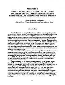
Proposition 1 suggests that θ(0, L) may be large if A(x) is large when x goes to w − L. A simple example, illustrated in Figure 1, is as follows. Assume L = w and (

u(x) =

1 − exp(−ax) if x ≤ xb b + cx if x > xb

where b = 1 − w exp(−axb)/(w − xb) and c = exp(−axb)/(w − xb), and xb is a fixed parameter such that 0 < xb < w. Thus u(0) = 0, u(w) = 1 and A(x) = a if x ≤ xb and A(x) = 0 if x > xb.2 When a is increasing (with a given value of xb), the individual becomes more risk averse in the neighbourhood of the bad outcome x = 0, with unchanged normalisation u(0) = 0, u(w) = 1. We then have Cp0 (0, L) = 1/c = (w − xb) exp(axb) and thus Cp0 (0, L) is increasing with a and it goes to infinity when a goes to infinity. Since xb is arbitrarily small, we learn from this example that Cp0 (0, L) may be large if the individual is highly risk averse in the neighbourhood of the loss state x = w − L, or equivalently if her risk tolerance is very small around this state. CRRA preferences are an instance of such a case with T (x) = γx, where γ is the index of relative risk aversion. We then have T (x) −→ 0 and A(x) −→ ∞ when x −→ 0. However, although CRRA preferences are quite useful for calculation tractability and calibration issues (see Section 4), they are not very satisfactory from a theoretical standpoint since the utility is not defined when wealth is nil. This corresponds to discontinuous preferences in which any lottery with zero probability for the zero wealth state is preferred to any lottery with a positive probability for this state. If preferences are of the HARA type, then risk tolerance is a linear function of wealth, and we may write T (x) = a + bx, with a > 0 and 0 < b < 1. In such a case, we have A0 (x) < 0, A(0) = 1/a and R(x) > 1. In particular, the individual’s absolute risk aversion index is decreasing but upper bounded. A straightforward calculation then gives !

1 bw 1 Zw A(x)dx = ln 1 + , 2w 0 2bw a and thus, Corollary 1 shows that for all M > 0, we have θ(0, L) > M if a
x b, but this is just for simplicity.

6

Figure 1: xˆ = 30, w = 100 if b = T 0 (x) is small enough. In words, the risk tolerance should be low in the neighbourhood of the catastrophic state x = 0 for the normalized risk premium θ(0, L) to be large3 . Proposition 2 establishes another sufficient condition under which θ(0, L) is (arbitrarily) large when the individual is sufficiently risk averse (or, equivalently, when her risk tolerance is sufficiently low) in the catastrophic loss state. Proposition 2 Assume T (x) ≡ Tε (x) = ε + t(x), with ε > 0, t(w − L) = t0 (w − L) = t00 (w − L) = 0, t0 (x) > 0 for x close to w − L. Then for all M > 0, there exists ε > 0 such that θ(0, L) > M if ε is small enough. In Proposition 2, it is assumed that the risk tolerance increases slowly (less than degree-two polynomials) when wealth x increases in the neighbourhood of w − L. In such a setting, the normalized risk premium may be arbitrarily large if the risk tolerance in the loss state ε is small enough. 3

We know that continuity of preferences among lotteries is one of the axioms that sustain the representation of preferences by the expected utility criterion.

7

2.2

Insurance demand for catastrophic risks

We now assume that the individual can purchase insurance for a small probability-large severity risk (p, L). Insurance contracts specify the indemnity I in the case of an accident, i.e., when the individual suffers the loss L, and the premium P to be paid to the insurer, with P = (1 + σ)pI, where σ > 0 is the loading factor such that p(1+σ) < 1. The policyholder then faces the lottery (w1 , w2 ), with corresponding probabilities (1 − p) and p, where w1 and w2 denote the wealth in the no-loss and loss states respectively, with w1 = w − P and w2 = w − P − L + I. A straightforward calculation shows that feasible lotteries are defined by [1 − p(1 + σ)]w1 + (1 + σ)pw2 = w − (1 + σ)pL,

(5)

with in addition w2 − w1 + L ≥ 0,

(6)

for the sign condition I ≥ 0 to be satisfied. The optimal lottery maximizes the individual’s expected utility (1 − p)u(w1 ) + pu(w2 ), in the set of feasible lotteries. It is such that the marginal rate of substitution −dw2 /dw1|Eu=ct. = (1 − p)u0 (w1 )/pu0 (w2 ) is equal to the slope (in absolute value) of the feasible lotteries lines, that is (1 − p)(1 + σ)u0 (w1 ) = [1 − (1 + σ)p]u0 (w2 ).

(7)

Figure 2 shows the locus of optimal lotteries in the (w1 , w2 ) plane when p changes. Point A represents the situation with no insurance and point B the represents the optimal lottery when p goes to zero. Equations (5) and (7) define the optimal state-contingent wealth levels w1 (p, L), w2 (p, L), when I > 0, that is when σ is not too large. Let us denote w1∗ (L) ≡

p−→0

w2∗ (L) ≡

p−→0

lim w1 (p, L) = w,

lim w2 (p, L),

with u0 (w2∗ (L)) = (1 + σ)u0 (w).

(8)

which implies w2∗ (L) < w = w1∗ (L). Thus, when p goes to 0, the optimal insurance contract (P, I) goes to a limit (P ∗ , I ∗ ), with P ∗ = 0 and I ∗ = 8

−3

Figure 2: w = 10000, L = 5000, u(x) = − x 3

w2∗ (L) + L − w1∗ (L) < L. When p is positive but close to 0, we still have I < L and P = (1 + σ)pI ' (1 + σ)pI ∗ . Since w2∗ (L) = w − L + I ∗ , (7) gives u0 (w − L + I ∗ ) = (1 + σ)u0 (w), or I ∗ = u0−1 ((1 + σ)u0 (w)) − w + L, and thus I ∗ is decreasing with σ. Finally, we may characterize the effect of a change in L and/or w on optimal insurance coverage. An increase dL > 0, for w given, induces an equivalent increase dI ∗ = dL. A simultaneous increase dw = dL > 0 induces an increase dI ∗ > 0 in coverage, while an increase in wealth with unchanged loss dw > 0, dL = 0 entails a decrease in optimal coverage dI ∗ < 0 under DARA references, i.e., when A0 < 0. Of course, there is nothing astonishing here. These are standard comparative statics results, which are extended here to the asymptotic characterization of catastrophic risk optimal insurance. They are summarized in Proposition 3.

9

Proposition 3 When p goes to 0, the optimal insurance coverage I goes to a limit I ∗ and when p is close to 0, coverage I and premium P are close to I ∗ and (1 + σ)pI ∗ , respectively. I ∗ is lower than L and it is decreasing with σ. A simultaneous uniform increase in L and w induces an increase in I and P . Under DARA, an increase in w, with L unchanged, induces a decrease in I and P .

3

Optimal catastrophic risk coverage for a population

With the case of nuclear accident risk in mind, we now consider a population of individuals who face the risk of a catastrophic event (called "the accident") caused by a firm. Such an accident may affect them differently, according to their risk exposure and also to their good or bad luck. The population has unit mass and it is composed of n groups or types indexed by i = 1, ..., n and a proportion αi of the population belongs to group i, with α1 + α2 + ... + αn = 1. In the case of a nuclear accident caused by a given reactor, the groups correspond to various locations that may be more or less distant from the nuclear power plant. The accident occurs with probability π. In the case of an accident, a proportion qi ∈ [0, 1] of type i individuals suffer damages, with financial damages xei for each individual in this subgroup of victims. xei is a random variable, whose realization is denoted xi , and which is distributed over the interval [0, xi ] with c.d.f. F (xi ) and density f (xi ) = F 0 (xi ). The random variables xei are independently distributed among type i individuals. Thus we assume that in group i, the victims are randomly drawn with probability qi and thus, because of the Law of Large Numbers, the proportion of affected individuals is equal to qi , while their damages are independently distributed. The total cost of an accident is equal to n X i=1

αi qi

"Z xi 0

#

xi f (xi )dxi =

n X

αi qi E xei .

i=1

Under our assumptions, this total cost is given, but the distribution of loss between members of each group is random. Each type i individual is covered from the risk of an accident by an insurance contract that specifies an indemnity Ii (xi ) ≥ 0 for all xi in [0, xi ]. This insurance coverage is taken out by the firm at price P . Once again with the nuclear liability law in mind, we assume that the firm has to indemnify the victims according to the legal rule Ii (xi ) and also - in order to prevent any bankruptcy risk - that it has to purchase insurance to cover its liability. 10

Thus Ii (xi ) is at the same time the payment by the firm to type i individuals and the transfer from the insurer to the firm. The firm pays a premium P per individual, and this premium is passed on to the prices of the firm’s product (say, on to the consumers’ electricity bill). We assume that all consumers purchase the same quantity of the firm’s products, and thus it is as if the insurance premium were paid by the individuals themselves. For the time being, P is defined as the firm’s expected liability cost, loaded at rate σ > 0. A more realistic formulation, with explicit capital cost, will be considered in a second stage. Thus, we have P = (1 + σ)π

n X

αi qi

"Z xi 0

i=1

#

Ii (xi )f (xi )dxi .

(9)

Let w1 and w2i (xi ) the wealth of a type i individual if she is not affected by an accident (which occurs with probability 1 − πqi ), and if she is affected with loss xi (which occurs with probability πqi and conditional loss density f (xi )) respectively. We have w1 = w − P, w2 (xi ) = w − P − xi + Ii (xi ). All individuals have the same initial wealth w and the same risk preferences represented by utility function u, with u0 > 0, u00 < 0. The certainty equivalent loss incurred by type i individuals is denoted by Ci . It is given by u(w − Ci ) = (1 − πqi )u(w1 ) +πqi

Z xi 0

u(w2 (xi ))f (xi )dxi .

(10)

The set of feasible lotteries {w1 , w21 (x1 ), ..., w2n (xn )} is defined by "

w1 1 − (1 + σ)π

n X

#

αi qi + (1 + σ)π

i=1

= w − (1 + σ)π

n X i=1

αi qi

n X i=1

"Z 0

αi qi

"Z xi 0

#

w2 (xi )f (xi )dxi

#

xi

xi f (xi )dxi ,

(11)

and w2i (xi ) − w1 + xi ≥ 0 for all i = 1, ..., n.

(12)

(11) and (12) can be derived as (5) and (6) in the simple one loss-one individual model. In particular, (12) corresponds to the positivity constraints Ii (xi ) ≥ 0. 11

We consider a utilitarian regulator that designs the risk coverage mechanism in order to minimize the social cost of an accident, which is the weighted sum of certainty equivalent individuals’ losses. This may be written as minimizing n X

αi Ci ,

i=1

with respect to {w1 , w21 (x1 ), ..., w2n (xn ); C1 , C2 , ..., Cn } subject to conditions (10),(11) and (12). Proposition 4 characterizes the optimal solution of this problem when π goes to 0. Proposition 4 When π goes to 0, all the optimal indemnity schedules Ii (xi ) converge towards a unique straight deductible schedule I ∗ (xi ) = max{xi − d∗ , 0}, where the deductible d∗ is given by u0 (w − d∗ ) = (1 + σ)u0 (w) with d∗ > 0. For π close to 0, we have P ≡ P (π) ' (1+σ)π

n P i=1

αi qi

hR xi 0

Proposition 4 shows that the optimal indemnity schedule for π small involves full coverage of the victims above a straight deductible d∗ (the same for all individuals whatever their type).4 This amounts to saying that the victims should be ranked in order of priority on the basis of their losses: the victims with loss xi should receive an indemnity only if the victims with loss x0i larger than xi receive at least x0i − xi . This simple characterization of optimal indemnification will be used in the simulation conducted in Section 4. As in the simple model of Section 2.1, we may derive comparative statics properties about the asymptotic deductible d∗ . In particular, it is increasing in σ and, under DARA preferences, it is increasing in wealth. The previous model goes through a very sketchy representation of the insurer’s costs: as usual for insurance pricing, we assumed that these costs where equal to the expected value of indemnities, marked up through the loading factor σ in order to take claims handling costs and various operating costs into account. In particular, the cost of capital allocation was not taken into account. In the case of low probability-high severity risks, capital allocation plays a major role and we should make it explicit in the definition of insurance costs. Assume that the insurer allocates an amount of capital per individual K in order to pay indemnities, should an accident occur. This is a contingent 4

The fact that the deductible does not depend on type i is true only asymptotically when π −→ 0. Otherwise, the optimal indemnity schedule involves type dependent deductibles di , with Ii (xi ) = max{xi − di , 0}. This is because lower deductibles would allow the regulator to transfer wealth from more risky types to less risky types (say from the groups with qi high to the groups with qi low if the conditional distribution of losses Fi (xi ) is the same for all groups). This compensatory effect vanishes when π goes to 0.

12

i

(xi − d∗ )fi (xi )dxi .

capital, i.e., an amount of resource brought by investors, held in a liquid form and that will be attributed to the insurer with probability π. A simple case (at least from a conceptual standpoint) is when the insurer issues a catbond with par value K. The catbond will pay some return (a spread above the risk-free rate of return) and it will be reimbursed to investors only if no accident occurs. Otherwise, the catbond will default and its proceeds will be used by the insurer to indemnify the victims. We know from the Law of large Numbers that the average indemnity paid to type i victims in the case of an accident is Z xi

Ii (xi )f (xi )dxi ,

0

and thus for the total indemnity payment to be financed through contingent capital, we need to have K=

n X

αi qi

Z xi 0

i=1

Ii (xi )f (xi )dxi ,

with capital cost c(π, K), with c0K > 0, c0K 2 ≥ 0, c0π > 0.5 Equivalently, we have Z n K=

X

xi

αi qi

i=1

0

[w2i (xi ) − w1 + xi ]f (xi )dxi .

(13)

Adding the cost of capital in the insurer’s cost gives P = (1 + σ)π

n X

αi qi

i=1

"Z xi 0

#

Ii (xi )f (xi )dxi + c(π, K).

Under these assumptions, the previous problem is modified by inserting c(π, K) as a supplementary component of insurance cost in the left-hand-side of equation (11) and by adding (13) as a new constraint, with K as a new variable. Proposition 5 Under costly capital resources, when π goes to 0, all the optimal indemnity schedules Ii (xi ) converge towards I ∗ (xi ) = max{xi −d∗ , 0}. The deductible d∗ and the contingent capital K are jointly defined by u0 (w − d∗ ) = [(1 + σ) + c0K (0, K)]u0 (w), and K=

n X i=1

αi qi

"Z xi d∗

# ∗

(xi − d )f (xi )dxi .

5

If contingent capital were levied through a catbond, then c(K, π)/K would the spread, i.e., the compensation per $ required by investors for running the risk of losing their capital with probability π. See Section 4 for further developments.

13

As previously, d∗ and K depends on σ and w, but now they are also affected by the marginal cost of capital. If the investors were risk neutral and perfectly aware of the probability of an accident, we would have c(π, K) = πK, i.e., the cost of contingent capital would just be equal to the risk premium that compensates the expected loss due to the default. We would have c0K (π, K) = π and thus c0K (0, K) = 0. In such a case, the cost of contingent capital would not affect the optimal indemnity schedule. However, as we will see in more details in Section 4 by looking at the example of the catbond market for low probability triggers, because of the aversion of investors towards risk or towards ambiguity, or for other reasons, it is much more realistic to write the cost of capital as c(π, K) = µ(π)πK, with µ(π) > 1. In particular, if µ(π) −→ ∞ when π −→ 0, we may have c0K (0, K) > 0. In that case, and that will be illustrated in Section 4, the cost of capital affects the optimal indemnity schedule.

4

Nuclear catastrophe coverage

In practice, the nuclear liability is regulated by the Paris (1960) and Brussels (1963) conventions in Europe and by the Price-Anderson act (1957) in the US. The liability is entirely channeled to the operator of the power plants but limited to a given amount. The Price-Anderson act forces the nuclear industry to secure a coverage of approximately 10 billion US dollars, while the Paris and Brussels conventions have recently been revised to bring the coverage to a minimum of 700 million euros. Our objective in this Section is to characterize the optimal level of coverage K, that the Government should provide for large scale nuclear accidents. The probability of a nuclear disaster is difficult to assess because we only have few data about it. This scarcity is of course a blessing for societies, but it prevents us from using the usual data analysis techniques. Neither the probabilities nor the extent of economic damages can be inferred with a reasonable degree of accuracy from past events. Instead, we have to rely on the analysis developed by nuclear safety specialists. In particular, the Probabilistic Safety Assessment (PSA) studies aim at understanding the odds and the stakes of a major accident along several dimensions: sanitary, environmental, economic, etc. Designed to improve prevention and the ex-post management of a crisis situation, they deliver as a by-product, useful information about the probabilities of different scenarios, analyzed in details in Dreicer et al.

14

(1995) and Markandya (1995). Additional studies from international agencies, such as the French Institute for Radioprotection and Nuclear Safety (IRSN,2013) and the Nuclear Energy Agency (NEA,2000) also develop the methodology for estimating the costs associated with the various accident scenarios predicted by the PSA. As in Eeckhoudt, Schieber and Schneider (2000), we make use of the aggregate information on costs and probabilities drawn from the PSA studies to construct individual lotteries. These lotteries are subsequently used to estimate the social cost of a nuclear accident and the optimal coverage.

4.1

The nuclear risk model

We consider the risk associated with a particular nuclear reactor. A large scale accident occurs with a probability π and the overall French population (60 million individuals) is divided into two groups, indexed by i = 1, 2. The most exposed individuals (i = 1) live within a radius smaller than 100km away from the power plant. These people, who form a group of 2 million, support a higher risk of sanitary consequences and also face the risk of loosing their properties in the midst of a large-scale accident. Group i = 2 therefore comprises 58 million people. In the case of an accident, a type i agent can face S different situations, each state s = 1, ..., S being characterized by a probability fis , with fi1 +fi2 + ... + fiS = 1. Losses can be either economic, environmental or sanitary. We monetize all of them by assuming that individuals dispose of an initial global wealth w, that incorporates health and wealth components. This wealth is multiplicatively impacted by a financial factor xfs as well as a health factor xhs 6 . Although the liability of a nuclear accident is supported by the operator of the power plant, we assume that the latter passes on the costs of coverage to the consumers of electricity. The total level of coverage K is the control variable for the social planner and a parameter for the consumers. It entitles the agent to receive an indemnity I(s, K) in state s. The indemnity schedule is determined so as to match the optimal insurance contract, which consists in a straight deductible as shown in Section 3. In a given state, claims are ranked in terms of severity and repaid layer by layer, so that the most impacted individuals are paid first and that all indemnified individuals end up with the same final wealth. 6

This is a crude but simple way to express the complementarity between health and wealth: the welfare gain of an increase in wealth is negatively affected if health worsens, and vice versa. See Finkelstein, Luttmer and Notowidigdo (2013) on this complementarity.

15

The insurance premium P (K) per individual is written as: n1 n2 29 X 1 X f1s I1 (s, K) + f2s I2 (s, K) + µπK P (K) = (1 + λ)π 30 s=1 30 s=1

!

where λ is a standard loading factor associated with claim handling cost and µπK is the cost of contingent capital levied by the insurer to sustain the indemnity payment should an accident occur. We would have µ = 1 if the investors who provide contingent capital were risk neutral and if there were no ambiguity about the probability of an accident. The example of catbond markets shows that the providers of contingent capital for catastrophic risk require spreads that are much larger than what should be expected from risk neutral investors. Beyond risk aversion, contingent capital providers may not be fully confident about the accident probability. Ambiguity aversion has been indeed put forward as an explanation of high equilibrium returns required by investors in catbond markets. Either because of risk aversion or ambiguity aversion, we expect that µ is much larger than one7 . Final wealth is then defined as: wsf (K) = wθ(1 − xfs )(1 − xhs ) + w(1 − θ) + I(s, K) − P (K) 1 − θ is the fraction of wealth that cannot be altered by the accident 8 . The optimal coverage minimizes the weighted sum of the certainty equivalent of the losses of the two groups, C1 (K) and C2 (K) respectively with: u(w − Ci (K)) = (1 − π)u(w − P (K)) + π

n X

f fis u(wis (K))

(14)

s=1

For the sake of numerical tractability, we specify a Constant Relative Risk Aversion (CRRA) utility function: u(w) =

w1−γ 1−γ

where γ is the index of relative risk aversion and γ = 0 characterizes a risk neutral individual. The literature has not settled a clear consensus on 7

Bantwal and Kunreuther (2000) suggest that ambiguity aversion, loss aversion, uncertainty avoidance as well as transaction costs due to legal and technical complexities may account for the reluctance of investment managers to invest in the catbond market, and thus for high expected returns in this market. 8 The worst case scenario is a fatal outcome. Even when this worst state materializes, we assume that the agent is able to retain a small fraction of her global wealth. We think of this as a general form of bequest. Perhaps legacy would be the appropriate term, since the global wealth w is not purely financial.

16

the value of this parameter. However, micro studies such as Levy (1994) and Szpiro (1986) have isolated a plausible range between 1 and 5, while macroeconomic studies such as Mehra and Prescott (1985) tend to find much higher values. We will therefore let this parameter vary within this plausible range and we will include γ = 0 as a consistency check.

4.2

Recovering the individual lotteries

The analysis we conduct is based on the PSA study realized for the power plant of Tricastin (France) by Dreicer et al. (1995). We use figures similar to Eeckhoudt et al. (2000) to calibrate our baseline scenario. Along the health dimension, a person can potentially be in three different states: dead, severe health effect, no health effect. Along the financial dimension, a person can be in only two states: either she is relocated and suffers the worst possible financial damage or she is not relocated and she shares the indirect costs with the entire society. The most serious consequences of the baseline scenario (scenario 1) are summarized in table 1. For the alternative scenarios, the losses remain the same but the probabilities being impacted by a severe adverse outcome increases. To these consequences, one must add a more diffuse Group Population Relocated Death Sanitary effects h=1 2 million 10,000 500 1000 h = 2 58 million 0 3000 6000 Table 1: scenario 1 economic cost that is more difficult to attribute to a particular individual. Such costs are qualified as indirect costs in Schneider (1998) and subsequent works, they are difficult to quantify and to attribute to a given individual. Examples of such costs are : loss of attractiveness of an impacted territory, loss in terms of image for the industrial sector, etc9 . The assumption that is made in the PSA study is that these costs are more or less already shared by all individuals in the economy. In the case of an accident, each person can potentially be in 6 distinct states however, individuals from group 2 are never relocated, so they can only be in three different states. The lotteries associated with the base-line scenario are given in tables 2 and 3 9

It may also be argued that there exist some gains, as the reconstruction activities may produce spillover effects on the entire economy. It is likely that these gains do not compensate the indirect losses but no study has been realized for the nuclear accident case. See Gignoux and Menéndez (2014) for the case of earthquake in India

17

State xfs s=1 1 s=2 z s=3 1 s=4 z s=5 1 s=6 z

xhs 1 1 0.2 0.2 0 0

f1s 1.2500e-06 2.4875e-04 2.5000e-06 4.9750e-04 4.9963e-03 9.9425e-02

Table 2: lotteries for type h = 1 State xfs s=1 z s=2 z s=3 z

xhs f2s 1 5.3571e-05 0.2 1.0714e-04 0 9.9984e-02

Table 3: lotteries for type h = 2 We consider alternative scenarios (2,3,4,5) by multiplying all the figures in table 1 by 2,3,4 and 5, keeping the total cost fixed at 200 billion euros. This is obtained by reducing the cost of minor financial losses (denoted by z in Tables 2 and 3) in such a way that the total losses remain unchanged10 . In order to calibrate the parameter θ, we follow Eeckhoudt et al. (2000) and set θ = 0.9775.

4.3

Optimal coverage under a constant cost of capital

Assessing the premium P (K) requires a calibration of the parameter µ, which reflects the cost of the capital needed to secure the available coverage K. One way to sustain this coverage is to issue a cat-bond, that defaults with a probability π. The principal is therefore lost by the investor when the accident occurs and is used to pay the claims. To the best of our knowledge, no cat-bond with an attachment probability as low as 10−5 has ever been issued, so it is difficult to know what price would be required by the markets in order to provide capital contingent on the occurrence of a large-scale nuclear accident. We therefore need to extrapolate such a price from our current understanding of contingent capital pricing. Suppose that a risk neutral investor is interested in buying a cat-bond. He agrees to provide a capital K. With a probability π, also called attachment probability, a contractually defined event occurs and triggers a loss of capital 10

For instance, type 1 individuals are in state s=3 when they suffer severe financial losses and minor health problems.

18

for the investor. Conditionally on the occurrence of the event, the fraction of the capital that is lost is distributed according to a probability density function g(t) = G0 (t). The expected percentage loss of the principal in case R1 of accident is therefore 0 tg(t)dt ∈ [0, 1]. When the trigger is not activated, the cat-bond pays a return R and the capital is returned to the investor. Provided that investors are risk neutral or if the cat-bond risk is fully diversifiable, absence of arbitrage opportunity should guarantee that: πK[1 −

Z 1

tg(t)dt] + (1 − π)K(1 + R) = (1 + r)K

0

where r is the market risk-free rate of return. For a small enough attachment probability π, the spread s := R−r, required by the investor for the cat-bond, is well approximated by: s=π

Z 1

tg(t)dt

(15)

0

The spread is therefore determined by the attachment probability and the conditional expected loss. Notice that a cat bond specifying that the capital is entirely lost whenever the trigger is activated has a conditional expected R1 loss 0 xg(x)dx = 1 and therefore yields a spread: s=π

(16)

Which would imply a constant parameter µ = 1. In this case, reinsurance through contingent capital becomes really interesting for the insured. Instead of paying a liquidity premium of the order of magnitude of a few percentages, she pays a return that has the same magnitude than the attachment probability. Let us assume that µ is a positive constant so that the spread s is a linear function of the attachment probability. Using equation (14), we are now able to simulate the risk premiums for individuals of both types i = 1 and i = 2. The social cost of nuclear risk is calculated as: 29 1 SC(K) = C1 (K) + C2 (K) 30 30 ∗ The optimal coverage K is simply the coverage that minimizes C(K). Each of the three figures 3a, 3b and 3c display function SC(K) for the five different scenarios and for two different hypothesis on the cost of contingent capital. The first set of curves, that flatten on the south-east part of the figures, represent the social cost under the assumption that there exist investors willing to provide contingent capital, for a spread equal to the attachment probability so µπ = 1. The highest of these five curves corresponds 19

to the most serious accident of scenario 5 and the lowest corresponds to the base-line scenario 1. The set of curves that increases on the right part of the graphs represent the social costs, under the assumption that the required spread is 20. We see clearly that an increase in K involves a trade-off between a more efficient risk coverage and higher insurance costs, particularly capital costs. We can also remark that the optimal coverage is much lower when the required spread is higher. This result is qualitatively obvious but the amplitude of the change suggests that µ is indeed a key parameter for the choice of a coverage level.

(a) µ = 1, 20 π = 10−4 (b) µ = 1, 20 π = 10−5 (c) µ = 1, 20 π = 10−6

Figure 3 The most interesting result is the following: Result 1 Ceteris paribus, a change in the attachment probability does not impact the choice of coverage, provided that the probability is small enough and that there exist an uncertainty-neutral investor willing to provide contingent capital. This result echoes proposition 4 from Section 3: when π goes to zero, the optimal indemnity schedule converges to a limit. Thus, it is not astonishing that the optimal coverage does not substantially change when π goes from 10−4 to 10−6 . It is of practical importance because the small amount of data available makes it difficult for experts to settle the debate about what is the right probability of a large scale accident. Our result underlies the fact that this should not matter for the choice of an optimal coverage, at least as long as the probability is small and that there exist investors willing to provide contingent capital for a spread that is linear in the attachment probability. The simulations reported on the figures correspond to a level of relative risk aversion of 2. The optimal values of coverage for the entire economy (K*60 million) for γ = 1, ..., 5 are given in tables 5 and 6. For a risk neutral individual γ = 0, the coverage choice is zero, whatever scenario is considered. This is what we expect since there is a positive factor loading. 20

4.4

Optimal coverage under a variable cost of capital

In order to asses empirically the link between attachment probability, expected loss and the spread of a cat-bond, we use data from the specialized information website Artemis11 , that lists the main catastrophe and Insurance Linked Securities (ILS) transactions realized since the inception of the ILS market in the mid-nineties. The database contains more than two-hundreds issues, some of which are decomposed in several tranches characterized by different levels of risk and therefore by different spreads. We only have complete information for 97 of the most recent tranches, that span a short interval of two years (2013-2014). This period of time is sufficiently short to avoid complications due to the variations of prices generated by the underwriting cycle. For these issues, we have Rinformation about both the attachment probability and the expected loss π 01 tf (t)dt = πE(l), expressed as a fraction of the principal K. We estimate a model12 of the form: log(si ) = β0 + β1 log(πE(l)i ) + εi A simple OLS procedure delivers the results in Table 4. Both parameters Estimates constant −1.1970∗∗∗ (−6.3434) log(πE(l)i ) 0.3912∗∗∗ (9.2760) R2 0.4727 −4 µ ˆ(10 ) 82.2702 −5 µ ˆ(10 ) 334.2048 µ ˆ(10−6 ) 1357.6 Table 4: OLS estimates are significant1314 at the usual levels so the estimation can be useful to extrapolate the expected spread for a cat-bond with a very low attachment 11

http://www.artemis.bm/ Lane and Mahul (2008) use a similar data set to estimate a linear relation. The issue with their model is that the positive intercept they find implies that a cat-bond with a null attachment probability delivers a positive spread, which prevents their model from being used to derive expected spreads for low attachment probabilities. 13 The t-statistics are reported in parenthesis below the estimates. 14∗∗∗ : significant at 1% level. 12

21

probability. If we consider a simple cat-bond, for which the capital is entirely transferred to the sponsor if the trigger is activated, then the expected loss conditional occurrence of the accident is one: E(l) = 1. The expected spread sˆ is therefore: (17) sˆ(π) = exp(β0 )π β1 The fit of this predicted spread is shown in Figure 4.

Figure 4 ˆ of our model as: We can now compute the expected parameter µ(π) sˆ(π) π = exp(β0 )π β1 −1

µ ˆ(π) =

(18)

which is a decreasing function of π 15 . 15

We saw earlier that the optimal coverage for a nuclear accident relies importantly on the value of this cost of capital. Indeed, if investors were neutral toward risk and ambiguity, we would expect the cost of coverage µ to be independent from the attachment probability π (equation 15). So when the probability π becomes small, the price of coverage becomes

22

We now use (18), to derive the the social cost. From left to right, figures 5a, 5b, 5c represent the social costs for π = 10−4 , 10−5 , 10−6 . We see that the optimal coverage K ∗ now depends on the attachment probability that is considered. Everything else held constant, an increase in the attachment probability increases the optimal coverage because µ, the spread per unit of probability decreases with π.

(a) π = 10−4

(b) π = 10−5

(c) π = 10−6

Figure 5 Result 2 The optimal choice of coverage K ∗ is a decreasing function of π if the investor requires a spread per unit of attachment probability that is decreasing in the probability. So π does matter after all. But the reason why it does is that the price of contingent capital per unit of probability varies with the attachment probability, probably because of some kind of ambiguity aversion from the provider of capital. The fact that optimal coverage decreases with the probability of occurrence of the accident is due to the pricing behavior of the provider of capital, not to the behavior of the individual with respect to risk. Additionally, it is worthy of interest that ambiguity affects the investor and the insured asymmetrically. The low probability of an accident guarantees that for a given cost µ, ambiguity does not affect coverage choices. Insured are affected by ambiguity only to the extent that it affects the price of their policies. Finally, let us discuss the numerical results obtained for the optimal coverage in the more realistic case where µ is a function of K. It is clear that these results depend a lot on the assumptions that are made about the coefficient of relative risk aversion and about the scenario that is considered. very small as well, making it worthy for the society to choose a fairly high level of coverage. It is likely however, that investors are not neutral toward ambiguity, and require a higher spread for events that have very low attachment probabilities because these events are the ones for which the attachment probability is the most uncertain. With this respect, it is not surprising that µ ˆ is decreasing in π.

23

We have assumed that the most serious accidents are characterized by more severe losses incurred by the victims (deaths, diseases and relocation), keeping constant the aggregate cost of the accident. To know what what scenario reflects best the risk of a nuclear accident is a technical question but the economic insight is the following: Result 3 Ceteris paribus, a collective risk should have a higher coverage when its consequences are more concentrated on a subset of individuals. This result is particularly salient because we have chosen a CRRA function that reflects the individual’s supposed extreme aversion to losses that bring her global wealth close to zero. It is an interesting empirical question whether this extreme aversion indeed reflects the true preferences of people, but similar results would hold for any concave function since for a given aggregate cost, a risk that only affects lightly the majority of people is associated with higher individual losses for a small but increasing number of individuals. Of course, this reasoning is only valid as long as the most exposed individuals receive a weakly higher weight in the social welfare function. After these important disclaimers about the sensitivity of our analysis to the parameters of the underlying model, we can safely state the following: Result 4 The central scenarios (π = 10−5 ) are characterized by optimal levels of coverages higher than the 700 million euros provided for by the 2004 revision of the Paris convention. For example, Table 8 shows that K ∗ should be equal to 1.12 billion euros if we consider scenario 1, an index of relative risk aversion γ = 2 and a probability of occurrence π = 10−5 . Higher values of γ and/or a more pessimistic loss scenario would lead to much higher values of K ∗ .

5

Conclusion

This paper develops a theory of optimal insurance for high severity-low probability events. Starting with a characterization of what is a catastrophic risk for an individual, we have then analyzed the optimal insurance scheme for a risk of catastrophic accident, generated by a productive activity, that can potentially affect a full population. This has lead us to apply this approach to the case of nuclear accident risk. We have shown that two parameters are key in the determination of the optimal coverage: the degree of risk aversion and the cost of the contingent capital used to insure the catastrophic risk. Our results suggest that the nuclear liability law could be more ambitious than what it currently is in France. Of course, insuring a large catastrophe 24

such as a nuclear accident without resorting to innovative tools that provide additional international diversification possibilities turns out to be too costly. This is mainly due to the high spatial correlation of individual risks, that forces the insurance system to immobilize large and costly amounts of reserves to provide for the thankfully unlikely catastrophe, where all agents are hit at the same time. Nevertheless, innovative and cheaper solutions can be worked out with the actors of the Insurance Linked Securities and Cat-bond markets.

25

6

Appendix

6.1

Proofs

Proof of Proposition 1 For notational simplicity, and without loss of generality, the proof is written in the case L = w. We have Cp0 (w, 0) =

u(w) − u(0) Z w u0 (x) = dx. u0 (w) 0 u0 (w)

Since u0 (x) = u0 (w) −

Z w

u00 (t)dt

x

for all x ∈ [0, w], we may write Cp0 (w, 0)

u0 (x) = w− dx 0 u0 (w) " # Z w Z w 00 u (t) = w− dt dx 0 x u0 (w) # Z w "Z w u0 (t) A(t) 0 = w+ dt dx, u (w) x 0 Z w

and thus " # u0 (t) 1 Zw Zw θ(0, L) = 2 A(t) 0 dt dx. w 0 u (w) x

Integrating by parts gives 1Z w u0 (x) θ(0, L) = k(x)A(x) 0 dx 2 0 u (w) where k(x) = 2x/W 2 , with Z w

k(x)dx = 1.

0

Thus there exists h0 less than 1 such that h0

Z w 0

k(x)

u0 (x) dx = 1, u0 (w)

26

and we have 1 Zw θ(0, L) = h(x)A(x)dx 2h0 0 1Z w h(x)A(x)dx. > 2 0 0

(x) where h(x) ≡ h0 k(x) uu0 (w) , with

Z w

h(x)dx = 1.

0

Proof of Corollary 1 When L = w, we have 1 Z w xu0 (x) θ(0, L) > A(x)dx, w 0 wu0 (w) from Proposition 1. Furthermore, we have d[xu0 (x)] = xu00 (x) + u0 (x) dx = −u0 (x)[R(x) − 1], and thus

d[xu0 (x)] ≤ 0 if R(x) ≥ 1. dx

We deduce

1Zw θ(0, L) > A(x)dx if R(x) ≥ 1. w 0 Proof of Proposition 2 For the sake of notational simplicity, the proof is written in the case L = w. Assume T (x) ≡ Tε (x) = ε + t(x), with ε > 0, t(0) = t0 (0) = t00 (0) = 0, t0 (x) > 0 for x > 0. Let M > 0. Then, for ε small enough, there exists x0 (M, ε) and x1 (M, ε) such that 0 < x0 (M, ε) < x1 (M, ε), Tε (x0 (M, ε)) = x20 (M, ε)/w2 M , Tε (x1 (M, ε)) ≤ x21 (M, ε)/w2 M Tε (x) < x2 /w2 M if x0 (M ) < x < x1 (M ), x0 (M, ε) −→ 0 when ε −→ 0, x1 (M, ε) −→ x∗1 (M ) > 0 when ε −→ 0. 27

Thus, we have Tε (x) ≤

x1 (M, ε)x , w2 M

A(x) >

w2 M , x1 (M, ε)x

or equivalently

if x0 (M, ε) < x < x1 (M, ε). Hence, we may write 1Z w θ(0, L) > k(x)A(x)dx 2 0 ! 1 Z x1 (M,ε) 2x w2 M > dx × 2 x0 (M,ε) w2 x1 (M, ε)x x1 (M, ε) − x0 (M, ε) = M× . x1 (M, ε) Since x0 (M, ε) −→ 0 and x1 (M, ε) −→ x∗1 (M ) when ε −→ 0, the right-handside of the previous inequality goes to M when ε −→ 0, and we deduce that θ(0, L) is larger than M for ε small enough. Proof of Proposition 4 Let γi , ξ and ϕi (xi ) be Kuhn-Tucker multipliers associated with (10),(11) and (12), respectively. First-order optimality conditions are written as αi − γi u0 (w − Ci ) = 0 for all i, (19) 0 γi πqi u (w2 (xi ))fi (xi ) − ξ(1 + σ)παi qi fi (xi ) + ϕi (xi ) = 0 for all i, (20) n X

" 0

γi (1 − πqi )u (w1 ) − ξ 1 − (1 + σ)π

−

i=1 0

#

αi qi

i=1

i=1 n Z xi X

n X

ϕi (xi )dxi = 0

(21)

ϕi (xi ) ≥ 0 and ϕi (xi ) = 0 if w2 (xi ) − w1 + xi > 0 for all i.

(22)

Let xi such that w2 (xi ) − w1 + xi > 0. Thus, we have ϕi (xi ) = 0 from (22) and then (20) gives γi u0 (w2 (xi )) = ξ(1 + σ)αi .

(23)

u0 (w2 (xi )) = ξ(1 + σ)u0 (w − Ci ).

(24)

(19) and (23) yield

28

Hence, if there exist x0i , x1i ∈ [0, xi ] such that w2 (x0i ) − w1 + x0i > 0 and w2 (x1i ) − w1 + x1i > 0, then we have u0 (w2 (x0i )) = u0 (w2 (x1i )), and thus, using u00 < 0 we deduce w2 (x0i ) = w2 (x1i ). Consequently, w2 (xi ) is constant in the set of xi such that w2 (xi )−w1 +xi > 0, and we may write w2 (xi ) = w1 − di , with di < xi for all xi in this set, with u0 (w1 − di ) = ξ(1 + σ)u0 (w − Ci ).

(25)

Now, let xi such that w2 (xi ) − w1 + xi = 0. Using (19),(20) and (23) allows us to write u0 (w2 (xi )) = u0 (w1 − xi ) ≤ ξ(1 + σ)u0 (w − Ci ), and using (24) and u00 < 0 we deduce xi ≤ di . Thus, we have established that there exists di that satisfies (25) and such that w2 (xi ) = w1 − di if xi > di , w2 (xi ) = w1 − xi if xi ≤ di .

(26) (27)

When π −→ 0, we have w1 −→ w and Ci −→ 0 from (11) and (10), respectively. (25) then gives di −→ d∗ for all i when π −→ 0, with u0 (w − d∗ ) = ξ(1 + σ)u0 (w).

(28)

(19) and (21) then imply (

lim

π−→0

1−ξ−

n Z xi X i=1 0

)

ϕi (xi )dxi = 0.

(29)

If di ≤ 0 we have w2 (xi ) − w1 + xi > 0 and thus ϕi (xi ) = 0 for all xi > 0, and thus Z xi ϕi (xi )dxi = 0. 0

29

If di > 0, we have ϕi (xi ) = 0 for xi > di , and thus using (19),(20) and (27) gives Z xi 0

ϕi (xi )dxi =

Z di 0

ϕi (xi )dxi

= −πqi αi

Z di " 0 u (w1

#

− xi ) − ξ(1 + σ) fi (xi )dxi . (30) u0 (w − Ci )

0

Observe that ξπ does no go to infinity when π −→ 0. Indeed, in such a case we would have ξ −→ ∞ when π −→ 0, which would contradict (29) because ϕi (xi ) ≥ 0. Since Ci −→ 0 when π −→ 0, (30) allows us to write lim

Z xi

π−→0 0

ϕi (xi )dxi =

lim − πqi αi

π−→0

Z di " 0 u (w1 0

#

− xi ) − ξ(1 + σ) fi (xi )dxi 0 u (w)

= 0. (29) then gives ξ −→ 1 when π −→ 0 and (30) yields u0 (w − d∗ ) = (1 + σ)u0 (w) > u0 (w), which implies d∗ > 0. Since Ii (xi ) = w2 (xi ) + xi − w1 , we deduce that Ii (xi ) −→ I ∗ (xi ) = max{xi − d∗ , 0} when π −→ 0. Proof of Proposition 5 Let η ≥ 0 be a Kuhn-Tucker multiplier associated with constraint (13). The notations are unchanged for other multipliers. Now, (20) should be replaced by γi πqi u0 (w2 (xi ))fi (xi ) − [ξ(1 + σ) + η]παi qi fi (xi ) + ϕi (xi ) = 0, for all i = 1, ..., n, and we also have η − ξc0K (π, K) = 0.

(31)

A straightforward adaptation of the proof of Proposition 4 shows that the optimal indemnity schedule still converges to a deductible contract I ∗ (xi ) = max{xi − d∗ , 0} when π goes to 0, but now d∗ is given by u0 (w − d∗ ) = [(1 + σ) + c0K (0, K)]u0 (w), and (20) gives K=

n X i=1

αi qi

Z xi d∗

(xi − d∗ )f (xi )dxi .

30

6.2 6.2.1

Figures µ as a constant

Figure 6: µ = 1, 20 π = 10−4

31

Figure 7: µ = 1, 20 π = 10−5

Figure 8: µ = 1, 20 π = 10−6

32

6.2.2

µ as a function of π

Figure 9: π = 10−4

Figure 10: π = 10−5

33

Figure 11: π = 10−6

34

6.3

Tables

The following tables summarize the numerical results of section 4. Each table presents the optimal coverage for a given set of hypothesis on the costs λ, µ of the insurance scheme, and on the probability of occurrence π of the accident. Within each table, we let the degree of risk aversion vary through the columns. The scenarios that are considered vary across lines. All results are expressed in euros. 6.3.1

µ as a constant

Scenario Scenario Scenario Scenario Scenario

1 2 3 4 5

γ=0 0.000e+00 0.000e+00 0.000e+00 0.000e+00 0.000e+00

γ=1 2.685e+10 5.385e+10 8.070e+10 1.076e+11 1.344e+11

γ=2 3.210e+10 6.285e+10 9.360e+10 1.244e+11 1.500e+11

γ=3 3.420e+10 6.630e+10 9.855e+10 1.307e+11 1.500e+11

γ=4 3.525e+10 6.825e+10 1.011e+11 1.340e+11 1.500e+11

γ=5 3.600e+10 6.930e+10 1.028e+11 1.361e+11 1.500e+11

γ=4 1.590e+10 3.195e+10 4.785e+10 6.390e+10 7.980e+10

γ=5 1.875e+10 3.750e+10 5.625e+10 7.500e+10 9.375e+10

Table 5: µπ = 1, λ = 0.3, π = 10−4 , 10−5 , 10−6

Scenario Scenario Scenario Scenario Scenario

1 2 3 4 5

γ=0 0.000e+00 0.000e+00 0.000e+00 0.000e+00 0.000e+00

γ=1 9.000e+08 1.800e+09 2.700e+09 3.450e+09 4.350e+09

γ=2 7.050e+09 1.395e+10 2.100e+10 2.805e+10 3.495e+10

γ=3 1.215e+10 2.445e+10 3.660e+10 4.875e+10 6.090e+10

Table 6: µπ = 20, λ = 0.3, π = 10−4 , 10−5 , 10−6

35

6.3.2

µ as a function of π

In the following tables, equation (18) is used to derive the cost of contingent capital from the probability of occurrence π. The assumption λ = 0.3 is maintained, but this assumption affects only marginally the numerical results. Scenario Scenario Scenario Scenario Scenario

1 2 3 4 5

γ=0 0.000e+00 0.000e+00 0.000e+00 0.000e+00 0.000e+00

γ=1 0.000e+00 0.000e+00 0.000e+00 0.000e+00 0.000e+00

γ=2 3.120e+09 6.240e+09 9.360e+09 1.256e+10 1.568e+10

γ=3 7.440e+09 1.488e+10 2.232e+10 2.976e+10 3.720e+10

γ=4 1.112e+10 2.224e+10 3.336e+10 4.448e+10 5.552e+10

γ=5 1.408e+10 2.816e+10 4.216e+10 5.624e+10 7.032e+10

γ=3 4.400e+09 8.720e+09 1.312e+10 1.752e+10 2.184e+10

γ=4 7.600e+09 1.520e+10 2.280e+10 3.048e+10 3.808e+10

γ=5 1.048e+10 2.088e+10 3.136e+10 4.184e+10 5.224e+10

γ=3 2.480e+09 4.880e+09 7.360e+09 9.760e+09 1.224e+10

γ=4 5.120e+09 1.024e+10 1.536e+10 2.048e+10 2.560e+10

γ=5 7.680e+09 1.544e+10 2.312e+10 3.080e+10 3.856e+10

Table 7: λ = 0.3,π = 10−4

Scenario Scenario Scenario Scenario Scenario

1 2 3 4 5

γ=0 0.000e+00 0.000e+00 0.000e+00 0.000e+00 0.000e+00

γ=1 0.000e+00 0.000e+00 0.000e+00 0.000e+00 0.000e+00

γ=2 1.120e+09 2.320e+09 3.440e+09 4.640e+09 5.760e+09

Table 8: λ = 0.3,π = 10−5

Scenario Scenario Scenario Scenario Scenario

1 2 3 4 5

γ=0 0.00e+000 0.00e+000 0.00e+000 0.00e+000 0.00e+000

γ=1 0.00e+000 0.00e+000 0.00e+000 0.00e+000 0.00e+000

γ=2 1.600e+08 3.200e+08 4.800e+08 6.400e+08 8.000e+08

Table 9: λ = 0.3,π = 10−6

36

7

Bibliography

References [1] Arrow K.J. and Lind R.C. (1970), Uncertainty and the evaluation of public investment decisions, The American Economic Review, Vol. 60, No. 3, pp. 364-378. [2] Bantwal, V.J. and Kunreuther, H.C. (2000), A catbond premium puzzle, Journal of Behavioral Finance, vol.1, No. 1, 76-91. [3] Eeckhoudt L., Schieber C. and Schneider T. (2000), Risk Aversion and the External Cost of a Nuclear Accident, Journal of Environmental Management, Vol. 58, pp. 109-117. [4] Dreicer M., Tort V., and Margerie H. (1995), The External Costs of the Fuel Cycle: Implementation in France, CEPN report R-238. [5] Finkelstein, A., Luttmer, E.F.P., and Notowidigdo, M.J. (2013), What good is wealth without health? The effect of health on the marginal utility of consumption, Journal of the European Economic Association, 11(S1), 221-258. [6] Gignoux, J., Menéndez, M. (2014). Benefit in the wake of disaster: Longrun effects of earthquakes on welfare in rural Indonesia. [7] IRSN (2013), Methodology applied by the IRSN to estimate the costs of a nuclear accident in France. Report PRP-CRI/SESUC/2013-00261. [8] Lane, M. and Mahul, O. (2008), Catastrophe Risk Pricing: An Empirical Analysis. World Bank Policy Research Working Paper Series. [9] Levy, H. (1994). Absolute and relative risk aversion: an experimental study. Journal of Risk and Uncertainty 8, 289-307. [10] Markandya, A. (1995). Externalities of Fuel Cycles ExternE Project. Report Economic Valuation: An Impact Pathway Approach. European Commission DG XII. [11] Mehra, R. and Prescott, E. C. (1985). The equity premium: a puzzle. Journal of Monetary Economics. 15, 145-161. [12] NEA (2000), Methodologies for Assessing the Economic Consequences of Nuclear Reactor Accidents, OECD Nuclear Energy Agency, Paris. 37

[13] Schneider T. (1998), Integration of the Indirect Costs Evaluation, CEPN Report No. 260. [14] Szpiro, G. (1986). Measuring risk aversion: an alternative approach. The Review of Economics and Statistics 68, 156-159.

38