2009 American Control Conference Hyatt Regency Riverfront, St. Louis, MO, USA June 10-12, 2009
ThC03.6
Optimal Kalman Filtering with Random Sensor Delays, Packet Dropouts and Missing Measurements Maryam Moayedi , Yeng Chai Soh, and Yung Kuan Foo, Member, IEEE Abstract— In this paper an optimal Kalman filter design problem is studied for networked stochastic linear discrete-time systems with random measurement delays, packet dropouts and missing measurements. Any of these three uncertainties in the measurement can occur in the network in the same run. Based on a Markov chain, we develop a unified/combined model to accommodate random delay, packet dropouts and missing measurements. Some simulation examples are presented to show the effectiveness of the proposed approach.
A
I. INTRODUCTION
S the result of the increasing development in communication networks, control and state estimation over network has attracted great attention during the past few years (see e.g. [9]). The feedback control systems wherein the control loops are closed through a real-time network are called networked control systems (NCSs) (see e.g. [6]). In a NCS, data typically travel through the communication networks from sensors to the controller and from controller to the actuators. As a direct consequence of the finite bandwidth for data transmission over networks, time-delay is inevitable in networked systems where a common medium is used for data transfers. This delay, either constant, time varying, or random, can degrade the performance of a control system if the design is done without due consideration given to the delay. In many instances it can even destabilize the system. In addition, some packets not only suffer transmission delay but, even worse, can be lost during transmission. This phenomena is known as ‘packet dropout’; see [2], [15] for some further discussions. In practical applications, there may also be a nonzero probability that an observation consists of noise only, i.e. the measurements contain missing observations. The missing observations can arise for a variety of reasons, see [1], [7], [4] and [16] for more detailed discussions. Hence sensor delays, packet dropouts and missing measurements are some of the challenging problems faced by control practitioners in NCS, [2]. The filtering problem for systems with any of these uncertainties has received much attention during the past
M. Moayedi is with Nanyang Technological University, Singapore. (e-mail:
[email protected]) Y.C. Soh is with Nanyang Technological University, Singapore. (e-mail:
[email protected]). Y.K. Foo is with LW Electrical and Mechanical Engineering Private Limited, Singapore (e-mail:
[email protected]).
978-1-4244-4524-0/09/$25.00 ©2009 AACC
few years. See [1], [3], [4], [5], [8], [10], [11], [12], [13], [14] for example. In most of the literature, the aforementioned uncertainties in data transmission networks are usually assumed to happen separately. Very few works have been reported regarding the filtering problem for NCSs with mixed uncertainties in the measurement transmission network. Recently in [15] the robust H ∞ estimation for uncertain systems with signal transmission delay and data packet dropout has been considered. However, in their approach, the filter designed is essentially a continuous-time design involving an event-driven zero-order hold (ZOH). In [16], the H ∞ filter design problem is studied for a class of networked systems where two kinds of incomplete measurements, namely measurements with random delay and measurements with stochastic missing phenomenon are simultaneously considered. To the best of our knowledge, the filtering problems for NCSs with three simultaneous mixed uncertainties, i.e. random sensor delay, packet dropout and uncertain observation (missing measurement), have not been investigated in the literature. This motivates our present work. In this paper, we consider the case where any of all three types of uncertain observations (sensor delay, packet dropout and missing measurement) may occur in a single run. To achieve this aim, we use a finite-state Markov chain to model the uncertain system whose state is to be estimated. The design of the optimal estimator is then obtained via minimizing the approximate expected estimation error covariance matrix. One advantage of this approach is that it allows us to handle precedence constraint. We also use Markov chain in simulation for the purpose of evaluating the performance of the filters designed. This permits us to impose precedence constraints and hence more realistically models the real situation. For example, if a measurement packet arrives at discrete time k , then it could not be arriving again at time k + 1 because a packet could not be arriving twice. The organization of the paper is as follows. In the next section, we model the complete uncertain system via Markov chain and we present the various state equations used to model the uncertain system with measurement delay, packet dropout and missing measurement. We also discuss how the approach proposed in this paper can be readily adapted to admit multiple-step sensor delays and packet dropouts. In section 3, we present our main result and we discuss how a linear time-invariant filter using the same approach may be found. In section 4, we give several
3405
examples. Finally in section 5 we give our conclusion.
(13)
II. PROBLEM FORMULATION Consider the following discrete time linear time-invariant state-space model: x ( k + 1) = Ax ( k ) + w( k ), x ( k ≤ 0) = x0 , (1)
⎡ A 0 0⎤ ⎡ I 0 0⎤ ⎢ ⎥ A3 ( k ) = I 0 0 , B3 ( k ) = ⎢ 0 0 0 ⎥ ⎢ ⎥ ⎢ ⎥ ⎣⎢ 0 0 0 ⎥⎦ ⎣⎢ 0 I 0 ⎦⎥
(14)
0
(15)
C 3 (k ) = [0
(2) z ( k ) = Cx ( k ) + v ( k ) where x(k ) is the state vector, z (k ) is the measured output, and w( k ) and v ( k ) are stationary, zero-mean Gaussian discrete-time white noise processes with covariance matrices: T
E[ξ ( k )ξ ( k )] = diag[ Λ w , Λ v ],
ξ (k )
[ wT (k )
D3 ( k ) = [ I
(16)
T
T
(3) E[ξ ( k )ξ ( r )] = 0, k ≠ r and the initial condition satisfying the Gaussian probability distribution with T
E[ x0 ] = 0, E[ x0 x0 ] = P0
(4)
We assume that the plant is stable and observable from the measured output z (k ) . Systems with mixed uncertainties in the measurement may be represented by model of the form: X ( k + 1) = Ar ( k ) X ( k ) + Br ( k )W ( k ), (5) y ( k ) = Cr ( k ) X ( k ) + Dr ( k ) [ 0
compatible
dimension
I ]W ( k ); I of
[ vT ( k )
with
T
v ( k − 1) ] T
T
and W ( k ) = [ w ( k ) T
T
v (k )
T
x (k )
(7)
T
v ( k − 1) ] . T
Let [ Aq ( k ), Bq ( k ), Cq ( k ), Dq ( k )], q = 1, 2, 3, 4, denote the
four models obtained for the systems with no uncertainty, sensor delay, uncertain observations and packet dropout, respectively, with the following system matrices: ⎡ A 0 0⎤ ⎡ I 0 0⎤ A1 ( k ) = ⎢ I
⎢ ⎣⎢C z
0
0⎥ ,
⎥ 0 0 ⎦⎥
C 1 (k ) = [Cz D1 ( k ) = [ I
B1 ( k ) = ⎢ 0
0]
0
0
⎢ ⎣⎢ 0 I
0⎥
(8)
⎥ 0 ⎥⎦
(9)
0 ] ; I of compatible dimensions with
v; (10) and
⎡A 0 A2 ( k ) = ⎢ I 0 ⎢ ⎢⎣ 0 C z
C 2 (k ) = [0
D2 ( k ) = [ 0
⎡ I 0 0⎤ 0 ⎥ , B2 ( k ) = ⎢ 0 0 0 ⎥ ⎥ ⎢ ⎥ 0 ⎥⎦ ⎢⎣ 0 0 I ⎥⎦
0⎤
Cz
0] ,
(17)
C 4 (k ) = [0
0
(18)
D4 ( k ) = [ 0
0]
I ],
(19)
Let the probability that the system at time k is given by [ Aq ( k ), Bq ( k ), Cq ( k ), Dq ( k )] be ρ q . 4
Obviously,
∑ ρq = 1 . q =1
For ease of illustrating the concept of precedence constraint and for purpose of simulation, we define the following conditional probability: Prob (system is given by [ Aq ( k ), Bq ( k ), Cq ( k ), Dq ( k )] at D j ( k − 1)] at time k − 1 ) = ρ q / j .
T
y (k )] T
⎡ A 0 0⎤ ⎡ I 0 0⎤ A4 ( k ) = ⎢ I 0 0 ⎥ , B4 ( k ) = ⎢ 0 0 0 ⎥ ⎢ ⎥ ⎢ ⎥ ⎢⎣ 0 0 I ⎥⎦ ⎢⎣ 0 0 0 ⎥⎦
time k given system was [ A j ( k − 1), B j ( k − 1), C j ( k − 1),
(6) where we have defined X ( k + 1) = [ x ( k + 1)
0 ] ; I of compatible dimensions with v ;
and
v (k )] , T
0] ,
(11)
(20) It then follows that given ρ q / j , ρ q may be computed from the following equation: 4
∑ ρq/ j ρ j j =1
ρq
It should be clarified that in our filter design, we do not require the knowledge of ρ q / j ’s, only the values of ρ q ’s are required for the computation of the filter. This is desirable as one can often make some good estimations of ρ q ’s by empirical observations, experimentations, and statistical analyses but not ρ q / j ’s. Remark 2.1: We note that precedence constraint may force some of ρ q / j ’s to be zero. Specifically, consider the case where y (l ) is given by z (l ) (i.e. the packet arrives corresponds to current measurement). Then the packet arrived at time l + 1 cannot be z (l ) again since a packet cannot arrive in two consecutive times and z (l ) has already arrived at k = l . Hence we may conclude ρ 2/1 = 0 .
(12)
I ] ; I of compatible dimensions with v ; 3406
Let [ Ar ( k ), Br ( k ), Cr ( k ), Dr ( k )] denote the “real” model
where Λζ ( k ) denotes the covariance matrix of ζ ( k ) . X is
of system at time k . We may then represent [ Ar ( k ), Br ( k ), Cr ( k ), Dr ( k )] as:
independent of xs . Hence its covariance matrix may be
[ Ar
Br
4
∑ α q [ Aq , Bq , Cq , Dq ]; ∑ α q = 1,
Dr ]
Cr
4
q =1
T
(21)
Obviously Prob{α q (k ) = 1} = ρ q (k ) and the covariance of 4
j =1
β j (k ) = 0 or 1
(22) (23)
Λ X , j (k ) gives the value of E{ X (k ) X T (k )} if the true
model
at
k −1
time
is
T
(24) which
j =2
j =2
+ B F ,q ΛW B F ,q , if q = 2 Then
the
covariance
matrix
(32a) of
ζ (k + 1)
is
4
Λζ ( k + 1) =
∑ α q (k )Λζ ,q (k + 1) . q =1
The probability of Λζ ( k + 1) given by Λζ ,q ( k + 1) is ρ q .
A. State Prediction Define
T
T
xs ( k ) ] T
⎡Λ w E[W ( k ) W ( k )] = ⎢ 0 ⎢ ⎢⎣ 0
(25)
⎤ 0 ⎥ ΛW ⎥ Λ v ⎥⎦ 0
Λv 0
[I
0
0
T
G s ( k ), As ( k )
Tr {Γ F Λ ζ ,q ( k + 1)Γ F } subject to (32) and (32a)
and
Γ 0 Λζ ,q ( k + 1)ΓT0 − Γ 0 Λ ζ ,q ,0 ( k + 1)ΓT0 = 0
(26)
The augmented plant-filter system may then be represented as: ζ ( k + 1) = AF ( k )ζ ( k ) + BF ( k )W ( k ) (27) e( k ) = Γ F ζ ( k ), Γ F
The problem of minimizing E[e ( k + 1)e( k + 1)] may be posed as min
0
T
−I ]
(28)
Note that (33) Λ ζ ,q ( k + 1) which
takes
care
⎤ ⎡ ⎤ , BF ( k ) = ⎢ ⎥ ⎥ (29) As ⎦ ⎣Gs Dr [ 0 I ]⎦ Br
Given As ( k ) and Gs ( k ) , the propagation of the covariance T
T
entries
T
Γ 0 Λ ζ ,q ( k + 1)Γ 0 − Γ 0 Λ ζ ,q , 0 ( k + 1)Γ 0 − ε I ≤ 0
of
(33a)
where ε is an arbitrarily small positive number to account for round-off errors in numerical implementation. Apply Schur complement transformation; the above minimization problem is equivalent to
matrices for ζ ( k ) may be described by the equation Λζ ( k + 1) = AF Λ ζ ( k ) AF + BF ΛW BF
those
Remark 3.1: For computational purposes, we replace (33) by (33a) below: T
0
of
(33)
is not affected by the choice of A s and G s .
where
⎡ ⎢G C ⎣ s r
4
∑ {E[ β j ] AF ,q Λζ , j (k ) AFT ,q } / ∑ E[ β j ] T
minimizes
III. MAIN RESULT
AF ( k ) =
(32)
4
Λζ , q ( k + 1) =
T
Ar
j =1
T
xs ( k ), k = 1, 2,...,
T
∑ {E[ β j ] AF ,q Λζ , j (k ) AFT ,q }
+ BF , q ΛW BF , q , if q ≠ 2 , or
E[e ( k )e( k )] where e( k ) = x ( k ) − xs ( k ) .
T
(31)
4
Λζ , q ( k + 1) =
[ A j ( k − 1), B j ( k − 1),
x s (0) to be determined
ζ (k ) = [ X (k ) Note that
T
if ( q ≠ 2 and j ≠ 1 ) Hence
We wish to construct a linear estimator of the form x s ( k + 1) = A s ( k ) x s ( k ) + G s ( k ) y ( k ); generate
Aq ( k ), B q ( k ), C q ( k )
replaced with
Λζ ,q / j ( k + 1) = A F ,q Λ ζ , j ( k ) A F ,q + B F ,q ΛW B F ,q
C j ( k − 1), D j ( k − 1)] .
to
0 ] has the same number of rows as X .
and D q ( k ) respectively. Then we may derive:
Prob{β q (k ) = 1} = ρ q (k − 1)
system
and Γ 0 = [ I
C r ( k ) and D r ( k )
E{ X (k ) X T (k )} = E{∑ β j (k )Λ X , j (k )} Λ X (k )
β j (k ) = 1, ∑ j =1
and AF ,0 and BF ,0 are given by (29) with As = 0 , Gs = 0 Let AF , q and BF , q given by (29), with Ar ( k ), Br ( k ) ,
X (k ) may be written as:
4
T
Λζ ,0 ( k + 1) = AF ,0 Λζ ( k ) AF ,0 + BF ,0 ΛW BF ,0
q =1
α q = 0 or 1
T
given by Γ 0 Λζ ,0 ( k + 1)Γ 0 , where
min
(30)
3407
Gs ( k ), As ( k )
T
Tr {Γ F Λ ζ ,q ( k + 1)Γ F } subject to
⎡ −Λζ ,q ( k + 1) ⎢ T M q (k ) ⎢ Φζ ,q ( k ) A F ,q ⎢⎣ B TF ,q
⎤ ⎥ 0 ⎥≤0 −1 −ΛW ⎥⎦
A F ,q Φ ζ ,q ( k )
B F ,q
−Φ ζ ,q ( k ) 0
(34)
⎡ −Λζ ,q ( k / k ) ⎢ Φ ( k ) AT ( k / k ) F ,q ⎢ ζ ,q ⎢⎣ BFT ,q ( k / k )
BF , q ( k / k ) ⎤
−Φ ζ , q ( k )
0
0
−ΛW
−1
(37) T
Φζ , q (k ) = ∑ E[ β j ]Λζ , j (k ) if q ≠ 2
(37a) where we have similarly defined Λ q ,0 ( k / k )
j =1
4
j =2
j =2
T
T
Φζ , q (k ) = ( ∑ {E[ β j ]Λζ , j (k )) / ∑ [ β j ] if q = 2 Γ 0 Λζ ,q ( k + 1)Γ 0 − Γ 0 Λ ζ ,q , 0 ( k + 1)Γ 0 − ε I ≤ 0
0 ⎤ ⎡ −Λζ ,q ,X ( k / k ) Φζ ,q ( k ) ⎢ Φζ ,q ( k ) −Φ ζ ,q ( k ) M q ,0 ( k / k ) 0 ⎥≤0 ⎢ ⎥ −1 −ΛW ⎥⎦ 0 0 ⎢⎣
(34a)
Λζ ,q ,0 (k + 1) is the minimum-trace Λζ ,q , X (k + 1) that satisfies the LMI below: A F ,q ,0 Φζ ,q ( k ) −Φζ ,q ( k ) 0
If we impose the bound T
; j , q = 1,2,3,4 Thus, we may use the following recursive equations to find a sub-optimal As (k ) , Gs (k ) and L(k ) :
⎤ ⎥ ≤ 0 C. Conceptual Algorithm 0 ⎥ −1 Initialization: −ΛW ( k ) ⎥⎦ Use initial condition equal to (35) B F ,q ,0
xs (0) = E[ x0 ] = 0
T
Γ 0 Λζ ,q ( k + 1)Γ 0 − Γ 0 Λ ζ ,q , 0 ( k + 1)Γ 0 − ε I ≤ 0
Λζ , q (k + 1)
that
satisfies
(34)
and
4
min
T
P0
0 0
0 0
Λv 0
0⎤ 0 ⎥⎥ ; q = 1,2,3,4 0⎥ ⎥ εI⎦
To incorporate measurement updates, we set I 0⎤ ⎡ AF ( k / k ) ⎢ ⎥, ⎣ L ( k )C r ( k ) I ⎦ BF ( k / k )
0 ⎡ ⎤ ⎢ L ( k ) D ( k ) [ 0 I ]⎥ ⎣ ⎦ r
(36) The corresponding condition to (34)-(34a) is then M q (k / k )
Λζ (0 / 0) = ∑ α q Λζ ,q (0 / 0)
(39)
xs (0 / 0) = xs (0) + L (0) y (0)
(40)
q =1
(35)
State Prediction: A s ( k ), G s ( k ), Λ ζ ,q ( k + 1) given by: 4
where we have assumed x(−1) = x(0) and y (−1) = v(−1) in deriving the above initial condition. B. Measurement Update
s.t. (37) and (37a).
4
Solve (34) to find Gs (k ) with the initial condition: P0
∑ ρ qTr{Γ F Λζ ,q (0 / 0)ΓTF } q =1
Γ 0 Λζ ,q ( k + 1)Γ 0 = Γ 0 Λ ζ ,q , 0 ( k + 1)Γ 0
⎡ P0 ⎢P 0 Λ q (0) = ⎢ ⎢0 ⎢ ⎣0
(38)
L (0), Λ q (0 / 0) given by:
(34a)
simultaneously must satisfy (subject to numerical round-off error): T
as the
minimum-trace Λ q ( k / k ) that satisfies
and
⎡ −Λζ ,q ,X ( k + 1) ⎢Φ (k )A T M q ,0 ( k ) F ,q ,0 ⎢ ζ ,q ⎢⎣ B F ,q ,0T
T
Γ 0 Λζ ,q ( k / k )Γ 0 − Γ 0 Λζ ,q ,0 ( k / k )Γ 0 − ε I ≤ 0
4
4
⎥≤0 ⎥ ⎥⎦
; q = 1,2,3,4
where
Then
AF , q ( k / k )Φ ζ ,q ( k )
min ∑ ρ qTr{Γ F Λζ , q ( k + 1)Γ F } s.t. (34) and (34a). T
q =1
xs ( k + 1) = As ( k ) xs ( k ) + Gs ( k ) y ( k )
(41)
Prediction Error Covariance Bound Update: 4
Λζ ( k ) = ∑ α q Λζ , q ( k )
(42)
q =1
Filter Gain Computation and Error Covariance Bound with Measurement Update: Update k to k + 1 L ( k ), Λ q ( k / k ) given by: 4
min
∑ ρ qTr{Γ F Λζ ,q (k / k )ΓTF }
s.t. (37) and (37a).
q =1
4
Λζ (k / k ) = ∑ ρ q (k ) Λ ζ , q ( k / k ) q =1
State Update with Measurement:
3408
(43)
xs ( k / k ) = xs ( k ) + L ( k ) y ( k )
T
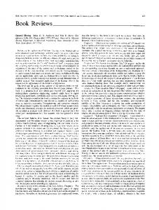
The result with xs (0) = [2 − 2] is depicted in figure 1-1
(44)
Remark 3.2: While ε is included in (35) to make Λ q (0) positive definite, in practice it may also be used t account for computational round-off errors. Remark 3.3: The above approach can be readily adapted to admit multiple-step sensor delays and packet dropouts by defining: X ( k + 1) = [ x ( k + 1) T
y ( k − 1) T
[
… T
W (k ) = w (k )
T
x (k )
…
x ( k − m) T
T
y (k )
T
y ( k − m)] T
T
v (k )
T
v ( k − 1)
...
v ( k − m − 1)
]
(46) where m is the maximum number of delay-steps that may occur. Note that we need to incorporate y (k ) , y (k − 1),..., y (k − m) as part of X (k + 1) because we need to account for the combined effect of both delays and packet dropouts, as well as precedence constraints. The number of LMI constraints we have to work with increases with the number of delayed steps allowed and this certainly would diminish the attractiveness of the approach if m is large. The alternative is to use an approximately optimal filter which we will be presented in a separate paper. IV.
z ( k ) = [1 1] x ( k ) + v ( k ) ; x (0) = [0 0]
T
(45) T
(with solid line depicting the real state, broken line depicting the state estimates). Example 2: In this example, we construct another filter for the following discrete-time LTI system [17]: ⎡ 0.8 0 ⎤ ⎡ 0.6 ⎤ ( ) x ( k + 1) = ⎢ x k + ⎥ ⎢ 0.5 ⎥ w( k ) ⎣ 0.9 0.2 ⎦ ⎣ ⎦ with the noise covariances Λ w = 1 and Λ v = 0.25 and ρ1 = 0.7 , measurement uncertainty probabilities ρ 2 = 0.045 , ρ3 = 0.085 and ρ 4 = 0.17 and we investigate its performance with the following conditional probabilities which are assumed for the system: ρ1/1 = 0.7 , ρ 2/1 = 0 , ρ3/1 = 0.1 , ρ 4/1 = 0.2 ; ρ1/ 2 = 0.7 , ρ 2/ 2 = 0.15 , ρ3/ 2 = 0.05 , ρ 4/ 2 = 0.1 ; ρ1/3 = 0.7 , ρ 2/3 = 0.15 , ρ3/3 = 0.05 , ρ 4/3 = 0.1 , ρ1/ 4 = 0.7 , ρ 2/ 4 = 0.15 , ρ3/ 4 = 0.05 and ρ 4/ 4 = 0.1 . The T
result with xs (0) = [2 − 2] is depicted in figure 2-1. As can be seen from the figures, the filter gives quite satisfactory performance for both systems with even high probability of measurement uncertainty.
EXAMPLE
x1
To illustrate the effectiveness of the proposed method, we present two examples for different systems and different uncertainty probabilities.
10
Example 1: In this example we consider the example of Sahebsara et al, [2]. We consider a discrete-time LTI system: ⎡1.7240 −0.7788 ⎤ ⎡1 ⎤ x ( k + 1) = ⎢ x ( k ) + ⎢ ⎥ w( k ) ⎥ 0 ⎦ ⎣ 1 ⎣0⎦
0
Actual state
-5 -10 -15
z ( k ) = [ 0.0286 0.0264 ] x ( k ) + 0.2 w( k ) ; x (0) = [0 0] Note that in their formulation, they have assumed the process noise and the measurement noise to be identical and hence we have also modified our formulation accordingly (the details are left to the Reader) to facilitate comparisons. In the simulation, we take the noise covariance equal to 1. We construct a filter based on a four-model uncertainty model with q = 1 (with probability ρ1 = 0.8 ), q = 2 T
(with ρ 2 = 0.02 ), q = 3 (with ρ3 = 0.09 ) and q = 4 (with ρ 4 = 0.09 ). (For notational simplicity, we shall denote a model using q = 1 , q = 2 , q = 3 and q = 4 as q = 1234 .) and then we evaluate its performance with q = 1234 simulation. The following conditional probabilities are assumed for the system: ρ1/1 = 0.8 , ρ 2/1 = 0 , ρ3/1 = 0.1 , ρ 4/1 = 0.1 ; ρ1/ 2 = 0.8 , ρ 2/ 2 = 0.1 , ρ3/ 2 = 0.05 , ρ 4/ 2 = 0.05 ; ρ1/3 = 0.8 , ρ 2/3 = 0.1 , ρ3/3 = 0.05 , ρ 4/3 = 0.05 , ρ1/ 4 = 0.8 , ρ 2/ 4 = 0.1 , ρ3/ 4 = 0.05 and ρ 4/ 4 = 0.05 .
Optimal filter
5
0
20
40 60 time step k
80
100
(a) x2 10 Actual state Optimal filter
5 0 -5 -10 -15
0
20
40 60 time step k
80
100
(b) Figure 1-1 Actual and estimated states for: (a) The first state; (b) The second state
3409
x1
[4]
3 Actual state
2
[5]
Optimal filter
1
[6]
0
[7]
-1
[8]
-2 -3
[9] 0
20
40 60 time step k
80
100
[10]
(a) x2 3
[11]
Actual state
2
Optimal filter
[12]
1 0
[13]
-1
[14]
-2 -3 -4 0
[15] 20
40 60 time step k
80
100
[16]
(b) Figure 2-1 Actual and estimated states for: (a) The first state; (b) The second state
[17]
V. CONCLUSION In this paper we have considered the optimal Kalman filtering problem where the measurements may be subject to random sensor delay, missing data and packet dropout in each run. Simulations are conducted to evaluate and demonstrate the performance of the proposed approach. The optimal filter is linear (whose gain does not depend on measurements) and may be pre-computed offline (and stored) before the filtering process begins. Given the present state of computing technology where memory costs are cheap (and getting cheaper and memory speed getting faster by leaps and bounds), the filtering scheme is, therefore, applicable in practice when the filtering timehorizon is not excessively long. For filtering time-horizon which is very long, the suitable choice is then the steadystate LTI filter. REFERENCES [1] [2] [3]
N.E. Nahi, ‘‘Optimal recursive estimation with uncertain observation’’, IEEE Trans. Inform. Theory, 15, p457–462, 1969. M. Sahebsara, T. Chen and S.L. Shah, “Optimal H2 filtering with random sensor delay, multiple packet dropout and uncertain observations,” Int. J. Control, 80, 2, 2007, p292-301. S. Sun, L. Xie, W. Xiao and Y.C. Soh, “Optimal estimation for systems with random measurement delays and packet dropouts’’, Automatica, 44, 5, p 1333-1342, 2008.
3410
Z. Wang, F. Yang, D.W.C. Ho and X. Liu, “Robust H∞ filtering for stochastic time-delay systems with missing measurement,” IEEE Trans. Signal Proc., 54, 7, p2579-2587, 2006. E. Yaz and A. Ray, ‘‘Linear unbiased state estimation under randomly varying bounded sensor delay’’, Appl. Math. Lett., 11, p 27–32, 1998. W. Zhang, M.S. Branicky and S.M. Phillips, ‘‘Stability of networked control systems’’, IEEE Cont. Mag., 21, p 84-99, 2001. Z. Wang, D.W.C. Ho, and X. Liu, ‘‘Variance-constrained control for uncertain stochastic systems with missing measurements’’, IEEE Trans. Sys., Man and Cybernetics, 35, 5, p 746-753, 2005. L. Zhang, Y. Shi, T. Chen and B. Huang, ‘‘A new method for stabilization of networked control systems with random delays’’, IEEE Trans. Automatic Cont., 50, p 1177-1181, 2005. J.P. Hespanha, P. Naghshtabrizi and Y. Xu, ‘‘A survey of recent results in networked control systems’’, IEEE Trans. Autom. Cont., 95, 1, p 138-162, 2007. M. Sahebsara, T. Chen, S.L. Shah, “Optimal H∞ filtering in networked control systems with multiple packet dropout’’, IEEE Trans. Automatic Cont., 52, 8, p 1508-1513, 2007. Z. Wang, F. Yang, D.W.C. Ho and X. Liu, “Robust finite-horizon filtering for stochastic systems with missing measurements’’, IEEE Trans. Signal Proc. Lett., 12, 6, p 437-440, 2005. O. Costa, “Stationary filter for linear minimum mean square error estimator of discrete-time Markovian jump systems ’’, IEEE Trans. Autom. Cont., 48, 8, p 1351-1356, 2002. S. Smith and P. Seiler, “Estimation with lossy measurements: Jump estimators for jump systems ’’, IEEE Trans. Autom. Cont., 48, 12, p 2163-2171, 2003. Z. Wang, D.W.C. Ho and X. Liu, “Robust filtering under randomly varying sensor delay with variance constraints’’, IEEE Trans. Circuits and Sys., 51, 6, p 320-326, 2004. H. Gao and T. Chen, “H∞ estimation for uncertain systems with limited communication capacity ’’, IEEE Trans. Autom. Control, 52, 11, p 2070-2083, 2007. X. He, Z. Wang and D. Zhou, “Robust H∞ filtering for networked systems with multiple state delays ’’, Int. J. Contr., 80, 8, 1217-1232, 2007. S. Sun, L. Xie, W. Xiao and N. Xie, “Optimal estimation for systems with multiple packet dropouts’’, IEEE Trans. Circuits and Systems, 55, 7, p 695-699, 2008.