Mar 30, 2012 - One example is given by data-rate constraints, whose study has led to ... over a digital error-free channel if and only if. R > âi max {0, log2 |λi(G)|} def. = HG,. (1) ... the measurements and encodes them for transmission over an ACGN ..... This will result in an increased cost, but this increase can be made ...
1
Optimal Linear Control over Channels with Signal-to-Noise Ratio Constraints
arXiv:1203.6741v1 [cs.SY] 30 Mar 2012
Erik Johannesson, Anders Rantzer, Fellow, IEEE, and Bo Bernhardsson
Abstract—We consider a networked control system where a linear time-invariant (LTI) plant, subject to a stochastic disturbance, is controlled over a communication channel with colored noise and a signal-to-noise ratio (SNR) constraint. The controller is based on output feedback and consists of an encoder that measures the plant output and transmits over the channel, and a decoder that receives the channel output and issues the control signal. The objective is to stabilize the plant and minimize a quadratic cost function, subject to the SNR constraint. It is shown that optimal LTI controllers can be obtained by solving a convex optimization problem in the Youla parameter and performing a spectral factorization. The functional to minimize is a sum of two terms: the first is the cost in the classical linear quadratic control problem and the second is a new term that is induced by the channel noise. A necessary and sufficient condition on the SNR for stabilization by an LTI controller follows directly from a constraint of the optimization problem. It is shown how the minimization can be approximated by a semidefinite program. The solution is finally illustrated by a numerical example. Index Terms—ACGN channel, control over noisy channels, linear-quadratic-Gaussian control, networked control systems, signal-to-noise ratio (SNR)
I. Introduction
C
OMMUNICATION limitations are a fundamental characteristic of networked control. The recent trend of decentralized and large-scale systems has therefore driven an interest in research on how control systems are affected by communication phenomena such as random time delays, packet losses, quantization and noise. A popular approach used for research on the fundamental aspects of communication limitations in control systems is to consider a plant that is controlled over a communication channel, as depicted in Fig. 1. Due to the lack of a theory that can handle all limitations at once, the channel model is typically chosen to highlight a specific issue. Submitted to the IEEE Transactions on Automatic Control on March 30th 2012. This work was supported by the Swedish Research Council through the Linnaeus Center LCCC; the European Union’s Seventh Framework Programme under grant agreement number 224428, project acronym CHAT; and the ELLIIT Strategic Research Center. The authors are with the Department of Automatic Control, Lund University, Box 118, 221 00 Lund, Sweden. Phone: +46 46 222 87 87. Fax: +46 46 13 81 18. E-mail: {erik, rantzer, bob}@control.lth.se. c
2012 IEEE. Personal use of this material is permitted. Permission from IEEE must be obtained for all other uses, in any current or future media, including reprinting/republishing this material for advertising or promotional purposes, creating new collective works, for resale or redistribution to servers or lists, or reuse of any copyrighted component of this work in other works.
Disturbance
Plant
Decoder
Channel
Encoder
Fig. 1. Feedback control of a plant, with disturbance, over a communication channel. The control system consists of an encoder, which also does measurement filtering, and a decoder, which also determines the control signal.
One example is given by data-rate constraints, whose study has led to one of the most well-known results in the area, known as the data-rate theorem. In discrete time, it says that an unstable linear plant G can be stabilized over a digital error-free channel if and only if X def max {0, log2 |λi (G)|} = HG , (1) R> i
where R is the rate of the channel and λi (G) is the ith pole of G [1], [2], [3]. The situation is more complicated for noisy channels. A necessary and sufficient condition for almost sure asymptotic stabilizability is that the channel capacity C satisfies C > HG [4]. But since this condition is not generally sufficient for mean-square stability, the concept of anytime capacity has been proposed for characterization of moment stabilizability [5]. Stability is, however, easier to characterize for control of a linear time-invariant (LTI) plant over an additive white Gaussian noise (AWGN) channel or, more generally, an additive colored Gaussian noise (ACGN) channel. Since the communication aspect highlighted by this channel model is a Signal-to-Noise Ratio (SNR) constraint, this setting will be referred to as the SNR framework. The SNR framework is mainly attractive due to its simplicity. However, it has been argued that the usage of linear controllers admits application of established performance and robustness tools [6]. The obtained results can sometimes also be used to draw conclusions about and design controllers for other communication limitations such as packet drops [7] or rate limitations [8], [9]. Moreover, the SNR framework can be useful for applications such as power control in mobile communication systems
2
[10]. A. Main Result and Outline This paper considers the problem of control design in the SNR framework. The system has the structure illustrated in Fig. 1. The plant is LTI, possibly unstable and subject to a Gaussian disturbance. The controller is based on output feedback and consists of an encoder and a decoder. The encoder measures the plant output, filters the measurements and encodes them for transmission over an ACGN channel. The decoder receives the channel output, decodes it and determines the control signal. The objective of the controller is to stabilize the system and minimize a quadratic cost function, while satisfying the SNR constraint. The main result is that an optimal LTI output feedback controller can be obtained by minimizing a convex functional and performing a spectral factorization. The minimization is performed over the Youla parametrization of the product of the encoder and the decoder, and the functional is the sum of the classical LQG cost and a new term that is induced by the channel noise. A condition for stabilizability, which coincides with the previously known condition in the AWGN case, is obtained as a constraint of the minimization problem. It is shown how to formulate the minimization as a semidefinite program. As a byproduct of the main result, it is also shown how the encoder and decoder should be chosen in order to minimize the impact of the channel noise while preserving the closed loop transfer function given by a nominal LTI controller that has been designed for a classical feedback system. The rest of this section will present the previous research in the SNR framework. Section II presents the mathematical notation used in this paper. The exact problem formulation is given in Section III. Section IV is devoted to the solution of the problem. Section V presents a procedure for numerical solution and a numerical example. Finally, Section VI presents the conclusions and discusses further research. Some technical lemmas have been put in the appendix. B. Previous Research Necessary and sufficient conditions for stabilizability, similar to the data-rate theorem, have been found for the SNR framework. They do, however, vary depending on some of the assumptions. Generally, the condition for the AWGN channel is that the SNR σ 2 satisfies the inequality ! Y 2 2 (2) | max{1, λi (G)}| − 1 + η + δ, σ > i
where η and δ depend on the specific assumptions, as will be explained. Assuming no plant disturbance and static state feedback, the condition is that (2) holds with η = δ = 0. By writing (1) and (2) in terms of the respective channel capacities, it can be shown that the capacity requirements for stabilization in the two settings are equal [6].
For LTI output feedback, the condition is again (2) but now the terms η and δ are non-negative and depend on the non-minimum phase zeros and the relative degree of the plant, respectively [6]. If there is a plant disturbance, the same condition holds if the controller has two degrees of freedom (DOF) [11] but not if it only has one DOF, in which case the required SNR is larger [12]. The condition with η = δ = 0 can be recovered for the output feedback case, either by introducing channel feedback, meaning that the encoder knows the channel output [11], or by allowing a time-varying controller, although the latter leads to poor robustness and sensitivity [6]. Further, it has been shown that the condition (2) with η = δ = 0 is necessary for stabilizability even if nonlinear and time varying state feedback controllers are allowed [13]. Similar conditions have been found for LTI control of a plant with no disturbance over an ACGN channel [12]. The case with first order moving average channel noise was further analyzed in [14]. An early formulation of a feedback control problem over an AWGN channel with feedback was made in [15]. It was shown how to find the optimal linear controller and that it is globally optimal for first-order plants. A counterexample was provided, showing that non-linear solutions may outperform linear ones for higher order plants [15]. It should, however, be noted that the provided counterexample requires the plant to be time-varying and that the encoder has a memory structure where it does not remember past plant output. Since then, many authors have considered similar control design problems that have been simplified by assumption of a certain controller structure, see [16], [17], [18], [19], [20]. A quite general approach was proposed in [11], but it was also noted that it leads to a difficult optimization problem with sparsity constraints when it is applied to controllers with two degrees of freedom. The problem of optimizing the control performance at a given terminal time was considered in [21] and [22]. The solutions may however yield poor transient performance and can therefore be unsuitable for closed-loop control. A lower bound on the variance of the plant state was obtained for feedback control over AWGN channels, using general controllers with two degrees of freedom, in [13]. This bound tends to infinity as the SNR approaches the limit for when stabilization is possible. An important contribution was recently made in [9]. Although the paper mainly considers control over a rate-limited channel, this is done through design of an LTI output feedback controller in the SNR framework, assuming an AWGN channel with feedback. The optimal performance is shown to be obtained by solving a convex optimization problem with the same structure as the one obtained in this paper. An optimal controller is then acquired by finding rational transfer functions that approximate certain frequency responses. Related results, for when the controller is pre-designed and the coding system should have unity transfer function, are given in [8] and [23].
3
Comparing with the results presented here, the case without channel feedback is not mentioned in [9]. The presented convex functional that gives the optimal cost for the case with channel feedback can, however, be modified to give the optimal cost for this case as well. The expressions for the optimal transfer functions that are given can, with additional work, also be modified to give solutions to the case without channel feedback. We claim that the solution presented in this paper has a clearer structure than the one given in [9]. For example, we do not require an over-parametrization of the controller. Moreover, while the plant is assumed to be single-input single-output (SISO) in [9], it is here allowed to be slightly more general, making it possible to include any number of noise and reference signals and to penalize the control signal variance. Also, we allow the channel noise to be colored. A final contribution of this paper relative to [9] is that it is shown how to pose the optimization problem as a semidefinite program. The approach used in this paper is based on the solution of a communication-theoretic problem involving design of encoders and decoders for a Gaussian source and a Gaussian channel when there is a delay constraint [24]. Some instances of that problem can be viewed as special cases (open loop versions) of the problem considered here, which therefore may be viewed as a partial generalization. II. Notation The proofs in this paper make extensive use of concepts from functional analysis, such as Lp (Lebesgue), Hp (Hardy) and N + (Smirnov) function classes and innerouter factorizations. To conserve space, only some of the most important facts will be given here. The interested reader is referred either to [25] or to [26], [27] and [28] for the remaining relevant definitions and theorems. The natural logarithm is denoted log. The complex unit circle is denoted by T. For matrix-valued functions X(z), Y (z) defined on T, define Z π � 1 tr X(eiω )∗ Y (eiω ) dω hX, Y i = 2π −π and the norms
Z π p 1 tr X(eiω )∗ X(eiω ) dω kXk1 = 2π −π �1/2 � Z π
1
X(eiω ) 2 dω kXk2 = F 2π −π � iω kXk∞ = ess sup σ1 X(e ) , ω
where k·kF is the Frobenius norm and σ1 the largest singular value. A transfer matrix X(z) is said to be proper if the mapping z 7→ X(1/z) is analytic at 0. It is strictly proper if also limz→∞ X(z) = 0. The space of all rational and proper transfer matrices with real coefficients is denoted by R. Lp , for p = 1, 2, ∞, is the space of matrix-valued functions X(z), defined on T, that satisfy kXkp < ∞.
v
z G
y
C
u
r
t
D
n H
w
Fig. 2. Feedback system with ACGN communication channel. The objective is to design the controller components C and D so that the plant G is stabilized and the variance of z is minimized under the SNR constraint E(t2 ) ≤ σ2 . H is a spectral factor of the channel noise n.
The subspaces RLp consists of all real, rational and proper transfer matrices with no poles on T. Hp , for p = 1, 2, ∞, is the space of matrix-valued functions X(z) such that z 7→ X(1/z) is analytic on the open unit disk and sup kXr kp < ∞, r>1
where Xr (z) = X(rz). The subspaces RHp consists of all real, rational, stable and proper transfer matrices. When a function in Hp is evaluated on T, it is to be understood as the radial limit limr→1+ X(rz). The arguments of transfer matrices will often be omitted when they are clear from the context. Equalities and inequalities involving functions evaluated on T are to be interpreted as holding almost everywhere on T. III. Problem Formulation A detailed block diagram representation of the system is shown in Fig. 2. The plant G is a multi-input multi-output (MIMO) LTI system with state space realization � � B1 B2 A Gzv (z) Gzu (z) G(z) = = C1 D11 D12 , Gyv (z) Gyu (z) C2 D21 0
where (A, B2 ) is stabilizable and (C2 , A) is detectable. The signals v and z are vector-valued with nv and nz elements, respectively. All other signals are scalar-valued. Accordingly, Gzv is nz × nv , Gyv is 1 × nv , Gzu is nz × 1 and Gyu is scalar and strictly proper. It is assumed that G∗zu Gzu and Gyv G∗yv have no zeros or poles on T. The input v is used to model exogenous signals such as load disturbances, measurement noise and reference signals. It is assumed that v and w are mutually independent white noise sequences with zero mean and identity variance. The other signals in Fig. 2 are the channel noise n, the control signal u, the measurement y and the control error or performance index z. The feedback system is said to be internally stable if no additive injection of a finite-variance stochastic signal
4
at any point in the block diagram leads to another signal having unbounded variance. This is true if and only if all closed loop transfer functions are in H2 . The communication channel is an ACGN1 channel with SNR σ 2 > 0. The channel noise has the spectral factor H ∈ RH∞ , which is assumed to have no zeros on T. Since the channel input and output can be scaled by C and D, it can be assumed that n has unit variance and thus 2 kHk2 = 1 without loss of generality. The SNR constraint is then equivalent to the power constraint E(t2 ) ≤ σ 2 .
2
2
2
2
CGyv
+ DCHGyu ≤ σ 2 ,
1 − DCGyu
1 − DCGyu 2
w2
Gyu u r
t
C
D
n Fig. 3.
Block diagram for internal stability analysis.
(3)
The objective is to find causal LTI systems C and D that make the system internally stable, satisfy the constraint (3) and minimize E(z T z) in stationarity. By expressing z and t in terms of the transfer functions in Fig. 2, the objective and the SNR constraint can be written as
2
DHGzu 2
DCGzu Gyv
+ J(C, D) = G +
1 − DCGyu
zv 1 − DCGyu
and
y
w1
(4)
2
respectively. The main problem of this paper is thus to minimize J(C, D) over C and D subject to (4) and internal stability of the feedback system. For technical reasons, only solutions where the product DC is a rational transfer function will be considered. This may exclude the possibility of achieving the minimum value, but the infimum can still be arbitrarily well approximated by such functions. Since D and C are required to be proper, DC has to be proper as well. That is, DC ∈ R. Though the latter will be enforced, it is not explicitly required that C and D are proper. It will, however, be seen that the solution is constructed so that C ∈ H2 is outer. Then C, C −1 are proper, and D = (DC)C −1 is also proper. IV. Optimal Linear Control The solution of the problem presented in the previous section is divided into three subsections. The first characterizes internal stability of the system. The second introduces the optimal factorization of a given nominal controller. The third section shows that the optimal factorization result can be used to find an equivalence between the main problem and the minimization of a convex functional in the Youla parameter. A. Internal Stability The product DC will play an important role in the solution. Therefore, introduce K = DC. 1 Since only linear controllers are considered, it does not matter if n or v are Gaussian or not. Linear solutions may, of course, be more or less suboptimal depending on their distributions.
Following the same reasoning as in [29], it is concluded that internal stability of the systems in Fig. 2 and Fig. 3 are equivalent (H does not have to be included since it is open-loop stable and not part of the feedback loop). The latter can be represented by the closed loop map T , defined by y w1 t = T w2 . u n
Hence, the system in Fig. 2 is internally stable if and only if KG Gyu DGyu yu 1 − KGyu 1 − KGyu 1 − KGyu C CGyu KGyu T = ∈ H2 . (5) 1 − KGyu 1 − KGyu 1 − KGyu KGyu D K 1 − KGyu 1 − KGyu 1 − KGyu The following two lemmas will give necessary and sufficient conditions for internal stability, respectively. Lemma 1: Suppose that T ∈ H2 , Gyu = N M −1 is a coprime factorization over RH∞ and that U, V ∈ RH∞ satisfy the Bezout identity V M + U N = 1. Then K=
MQ − U , NQ + V
Q ∈ RH∞ .
(6)
Proof: It follows directly from (5) that Gyu ∈ H2 , 1 − KGyu
K ∈ H2 , 1 − KGyu
1 ∈ H2 . 1 − KGyu
These transfer functions are rational and have no poles on or outside the unit circle, so it follows that 1 K � �−1 1 − KGyu 1 − KGyu 1 −K ∈ RH∞ , = Gyu 1 −Gyu 1 1 − KGyu 1 − KGyu (7) The set of K satisfying (7) can be parametrized using the Youla parametrization of all stabilizing controllers [29]. That is, K can be written as in (6). Lemma 2: Suppose that K = DC =
MQ − U , NQ + V
Q ∈ RH∞ ,
(8)
where Gyu = N M −1 is a coprime factorization over RH∞ and U, V ∈ RH∞ satisfy the Bezout identity V M +U N =
5
v
z G
y
u
K Fig. 4.
and
Classical feedback system without communication channel.
1. Suppose also that C ∈ H2 is outer and that D ∈ L2 . Then T ∈ H2 . Proof: It follows from (8) that Gyu K ∈ RH∞ , ∈ RH∞ , 1 − KGyu 1 − KGyu KGyu 1 = − 1 ∈ RH∞ . 1 − KGyu 1 − KGyu Moreover, KGyu DGyu = C −1 , 1 − KGyu 1 − KGyu where the left hand side is in L2 since it is the product of an L2 function and a RH∞ function. Since C is outer, application of Lemma 7 (in the appendix) gives that the right hand side is in H2 . A similar argument shows that D ∈ H2 . 1 − KGyu
Finally, C ∈ H2 , 1 − KGyu
Rewriting J(C, D) and the SNR constraint (4) with DC replaced by K gives
2
DHGzu 2 KGzu Gyv
J(C, D) = G + + (9)
zv 1 − KGyu
1 − KGyu 2 2
CGyu ∈ H2 , 1 − KGyu
since these functions are products of an H2 function and an RH∞ function. Since RH∞ ⊆ H2 it has been proved that all elements of T are in H2 and so T ∈ H2 .
CGyv 2 KHGyu 2 2
+
1 − KGyu ≤ σ .
1 − KGyu 2
The objective of the optimal factorization problem is to find C and D such that (9) is minimized subject to (10) and K = DC. Stability is not considered now but it will be seen that the obtained solution is stabilizing anyway. The optimal factorization will later be used to solve the main problem of this paper. Alternatively, it could also be used to factorize a nominal K that was designed for the classical feedback architecture. Note that, for given K, the first term in (9) is constant and that the second term is a weighted norm of D. In the left hand side of (10), the first term is a weighted norm of C and the second is constant. Thus, the optimal factorization problem is a minimization of a weighted norm of D, subject to an upper bound on a weighted norm of C and the constraint K = DC. Before the solution to this problem is given, it is noted that the SNR constraint will be impossible to satisfy unless K satisfies
KHGyu 2 def 2
≥ 0. α = σ − 1 − KGyu 2
Actually, if α = 0 then, since Gyv G∗yv has no poles or zeros on T,
2
CGyv C KHGyu
1 − DCGyu = 0 ⇒ 1 − DCGyu = 0 ⇒ 1 − KGyu = 0, 2
which is a contradiction. Thus, it will be assumed that K is such that α > 0. Introducing S=
B. Optimal Factorization Suppose for now that K ∈ R is a given stabilizing controller for the classical feedback system in Fig. 4. Thus, K satisfies (6). Nothing else is assumed about the design of K. It could for example be the H2 optimal controller or have some other desirable properties in terms of step responses or closed loop sensitivity. In either case, it is a natural question to ask what the best way is to implement this controller in the architecture of Fig. 2. If the nominal design is to be preserved then C and D should satisfy K = DC since the transfer matrix from v to z would then be the same. Given this relationship, choosing C and D can be thought of as factorizing K. The factorization should be chosen to minimize the negative effect of the communication channel. That is, they should keep the system stable, satisfy the SNR constraint and minimize the impact of the channel noise. That is, to minimize the contribution of n to E(z T z).
(10)
2
1 ∈ RH∞ 1 − KGyu
for notational convenience, the set of feasible pairs (C, D), parametrized by K, is defined as n o 2 ΘC,D (K) = (C, D) : kCSGyv k2 ≤ α, DC = K .
The solution to the optimal factorization problem is now given by the following lemma. Lemma 3 (Optimal Factorization): Suppose α > 0, S ∈ RH∞ , K ∈ R and that H ∈ RH∞ , G∗zu Gzu ∈ RL∞ and Gyv G∗yv ∈ RL∞ have no zeros on T. Then
1
KS 2 HGzu Gyv 2 . 1 α (11) Suppose furthermore that K ∈ RL1 satisfies (6). Then there exists (C, D) ∈ ΘC,D (K) with C ∈ H2 outer and D ∈ L2 , such that the minimum is attained and (11) holds with equality. inf
(C,D)∈ΘC,D (K)
2
kDSHGzu k2 ≥
6
If K is not identically zero, then (C, D) is optimal if and only if DC = K and s α G∗zu Gzu 2 |C| = |KH| on T. (12) 2 kKS HGzu Gyv k1 Gyv G∗yv If K = 0, then the minimum is achieved by D = 0 and 2 any C that satisfies kCSGyv k2 ≤ α. Proof: If K = 0 then the right hand side of (11) is 0. 2 Letting D = 0 gives kDSHGzu k2 = 0 and it is clear that (C, D) ∈ ΘC,D if C is as stated. Thus, it can now be assumed that K is not identically zero. Then C is not identically zero and D = KC −1 . By assumption both G∗zu Gzu and Gyv G∗yv are positive on the unit circle. Since these functions are rational this implies that ∃ε > 0 such that G∗zu Gzu ≥ ε and Gyv G∗yv ≥ ε, on T. (13) Thus by the factorization theorem in [30] there exist scalar ˆ zu , G ˆ yv ∈ H2 such minimum phase transfer functions G that ˆ∗ . ˆ∗ G ˆ zu , ˆ yv G G∗ Gzu = G Gyv G∗ = G zu
Now, gives
kCSGyv k22
zu
yv
yv
≤ α and Cauchy-Schwarz’s inequality
2
2 ˆ zu kDSHGzu k2 = KC −1 SH G
2
2
ˆ yv
2
CS G 2 ˆ zu ≥
KC −1 SH G
α 2 E2 D 1 −1 ˆ ˆ ≥ CS Gyv , KC SH Gzu α
2 1
ˆ yv ˆ zu G = KS 2 H G
α 1
1 2 = KS 2 HGzu Gyv 1 . α This proves the lower bound (11). ˆ zu | and Equality holds if and only if |KC −1 SH G ˆ yv | are proportional on the unit circle and |CS G 2 kCSGyv k2 = α. It is easily verified that this is equivalent to (12). Thus, (C, D) achieves the lower bound if and only if D = KC −1 and (12) holds, since these conditions imply that (C, D) ∈ ΘC,D (K). Under the additional assumptions that K ∈ RL1 satisfies (6), it will now be shown that there exists such (C, D) ∈ H2 × L2 with C outer. Since K satisfies (6) with M, N, Q, U, V ∈ RH∞ it holds that log |K| = log |M Q − U | − log |N Q + V | By Theorem 17.17 in [27], log |M Q − U | ∈ L1 and log |N Q + V | ∈ L1 and thus log |K| ∈ L1 . It follows from ˆ yv and G ˆ zu on T that (13) and the boundedness of H, G Z π G ˆ zu KH dω > −∞ log ˆ Gyv −π and
G ˆ zu KH ∈ L1 . ˆ yv G
Then by the factorization theorem in [30] there exists an outer function C ∈ H2 such that (12) holds. Also, D = KC −1 ∈ L2 since
ˆ yv
2 K G 1
2 −1
KC = KS HGzu Gyv
< ∞. 1 2 ˆ zu α HG 1
Remark 1: The spectral factorization gives some freedom in the choice of (C, D) that attains the bound. For example, D instead of C could be chosen to be H2 and outer. That would result in having C ∈ L2 . Considering more solutions than the one selected would require a slightly more complicated stability characterization, so this is not done. Remark 2: Optimal D will satisfy
s
KS 2 HGzu Gyv Gyv G∗yv K 2 1 on T. |D| = α G∗zu Gzu H
It is interesting that the magnitudes of both C and D are directly proportional, on the unit circle, to the square root of the magnitude of K. In other words, the dynamics of a nominal controller K is "evenly" distributed on both sides of the communication channel. The static gain of C (and D) is tuned so that the SNR constraint is active. In the case when Gyv = Gzu , finding an optimal factorization amounts to performing a spectral factorization of |KH| and tuning the static gain. If also H = 1 then the magnitudes of the frequency responses of C and D will then be proportional. C. Equivalent Convex Problem
It will now be shown that a solution to the main problem can be obtained, with arbitrary accuracy, by solving a convex minimization problem in the Youla parameter. As discussed in the problem formulation, (C, D) should satisfy the SNR constraint (4) and stabilize the system. The latter corresponds to T ∈ H2 or (5). Also, it was assumed that DC ∈ R. Thus, the set of feasible (C, D) is given by ΘC,D = {(C, D) : DC ∈ R , (4), T ∈ H2 } . Let M, N, U, V be determined by a coprime factorization of Gyu and introduce A = M 2 Gzu Gyv
(14)
2
B = M N V Gzu Gyv E = MNH
(15) (16)
F = (M V − 1)H
(17)
−1
L = Gzv − M N
−1
Gzu Gyv .
(18)
It will now be shown that minimization of J(C, D) over ΘC,D can be performed by minimizing the convex functional 2
ϕ(Q) = kL + AQ + Bk2 +
2
k(AQ + B) (EQ + F )k1 σ 2 − kEQ + F k22
,
7
over the convex set o n 2 ΘQ = Q : Q ∈ RH∞ , kEQ + F k2 < σ 2 .
The inequality in this definition is strict because it was shown earlier that equality cannot hold. It has thus been proved that
The Q ∈ ΘQ obtained from minimizing ϕ(Q) will be used to construct (C, D) ∈ ΘC,D . However, this will not be possible for Q for which the corresponding K has poles on T. For such Q a small perturbation can then be applied first. This will result in an increased cost, but this increase can be made arbitrarily small. That this is possible is established by the following lemma. Lemma 4: Suppose Q ∈ ΘQ and ε > 0. Then there ˆ ∈ ΘQ such that exists Q K=
ˆ−U MQ ∈ RL1 , ˆ+V NQ
(19)
and ˆ < ϕ(Q) + ε. ϕ(Q) The proof of Lemma 4 is based on a perturbation argument and can be found in the Appendix. The main theorem of the paper can now be stated. Theorem 1: Suppose σ 2 > 0, that Gyu = N M −1 is a coprime factorization over RH∞ , that U, V ∈ RH∞ satisfy the Bezout identity V M + U N = 1 and that H ∈ RH∞ , G∗zu Gzu ∈ RL∞ and Gyv G∗yv ∈ RL∞ have no zeros on T. Then inf
(C,D)∈ΘC,D
J(C, D) = inf ϕ(Q). Q∈ΘQ
(20)
ˆ ∈ ΘQ be Furthermore, suppose Q ∈ ΘQ , ε > 0 and let Q as in Lemma 4. Then there exists (C, D) such that the following conditions hold: ˆ − U is not identically zero: (C, D) ∈ H2 × L2 , • If M Q where C is outer and ˆ−U MQ K= (21) ˆ+V NQ
KHGyu 2 2
s
σ − 1 − KGyu 2 G∗zu Gzu 2
|KH| on T |C| =
KHGzu Gyv Gyv G∗yv
(1 − KGyu )2 1
D = KC
−1
(22)
(23)
ˆ − U = 0: C = D = 0. If M Q If (C, D) satisfy these conditions, then (C, D) ∈ ΘC,D and •
J(C, D) < ϕ(Q) + ε. Proof: Consider (C, D) ∈ ΘC,D and define K = DC. Then (C, D) ∈ ΘC,D (K) for this choice of K. Moreover, because T ∈ H2 it follows from Lemma 1 that K can be written using the Youla parametrization (6). Since the SNR constraint (4) is satisfied by (C, D) it follows that K ∈ ΘK , where ΘK is defined by ) (
KHGyu 2 2