Optimal Loop Unrolling For GPGPU programs - OhioLINK ETD

Optimal Loop Unrolling For GPGPU programs Thesis Presented in Partial Fulfillment of the Requirements for the Degree Master of Science in the Graduate School of The Ohio State University

By Giridhar Sreenivasa Murthy, B.E Graduate Program in Computer Science and Engineering

The Ohio State University 2009

Thesis Committee: Dr. P. Sadayappan, Adviser Dr. Atanas Rountev

c Copyright by

Giridhar Sreenivasa Murthy 2009

ABSTRACT

Graphics Processing Units (GPUs) are massively parallel, many-core processors with tremendous computational power and very high memory bandwidth. GPUs are primarily designed for accelerating 3D graphics applications on modern computer systems and are therefore, specialized for highly data parallel, compute intensive problems, unlike general-purpose CPUs. In recent times, there has been significant interest in finding ways to accelerate general purpose (non-graphics), data parallel computations using the high processing power of GPUs. General-purpose Programming on GPUs (GPGPU) was earlier considered difficult because the only available techniques to program the GPUs were graphics-specific programming models such as OpenGL and DirectX. However, with the advent of GPGPU programming models such as NVIDIA’s CUDA and the new standard OpenCL, GPGPU has become mainstream.

Optimizations performed by the compiler play a very important role in improving the performance of computer programs. While compiler optimizations for CPUs have been researched for many decades now, the arrival of GPGPU, and it’s differences in architecture and programming model, has brought along with it many new opportunities for compiler optimizations. One such classical optimization is ’Loop Unrolling’.

ii

Loop unrolling has been shown to be a relatively inexpensive and beneficial optimization for CPU programs. However, current GPGPU compilers perform little to no loop unrolling.

In this thesis, we attempt to understand the impact of loop unrolling on GPGPU programs and using this understanding, we develop a semi-automatic, compile-time approach for identifying optimal unroll factors for suitable loops in GPGPU programs. In addition, we also propose techniques for reducing the number of unroll factors evaluated, based on the characteristics of the program being compiled and the device being compiled to. We use these techniques to evaluate the effect of loop unrolling on a range of GPGPU programs and show that we correctly identify the optimal unroll factors, and that these optimized versions run up to 50 percent faster than the unoptimized versions.

iii

ACKNOWLEDGMENTS

I would like to thank my adviser, Professor P. Sadayappan for his advice and guidance throughout the duration of my Masters study. He has been a huge inspiration since my first CSE 621 class. I would also like to thank Professor Nasko Rountev for agreeing to serve on my Master’s examination committee. He has helped me immensely with his constant support and advice.

I would like to thank my colleagues in the HPC lab and other friends at OSU for their help and support. I would also like to extend my gratitude to the staff in the CSE Department at OSU for making my stay very pleasant.

I would like to specially thank Shilpa, my parents, my sisters and my niece for their constant motivation and encouragement, without which I would not have pursued my Masters.

iv

VITA

2000 - 2004 . . . . . . . . . . . . . . . . . . . . . . . . . . . . . . . . . B.E., Information Science and Engg, Visvesvaraya Technological University, Belgaum, India. 2004 - 2007 . . . . . . . . . . . . . . . . . . . . . . . . . . . . . . . . . Software Engineer, IBM India. 2007 - 2009 . . . . . . . . . . . . . . . . . . . . . . . . . . . . . . . . . Graduate Research Associate, The Ohio State University. 2008 . . . . . . . . . . . . . . . . . . . . . . . . . . . . . . . . . . . . . . . . Summer Intern, Advanced Micro Devices.

FIELDS OF STUDY Major Field: Computer Science and Engineering Studies in High Performance Computing: Prof. P. Sadayappan

v

TABLE OF CONTENTS

Page Abstract . . . . . . . . . . . . . . . . . . . . . . . . . . . . . . . . . . . . . . .

ii

Acknowledgments . . . . . . . . . . . . . . . . . . . . . . . . . . . . . . . . . .

iv

Vita . . . . . . . . . . . . . . . . . . . . . . . . . . . . . . . . . . . . . . . . .

v

List of Tables . . . . . . . . . . . . . . . . . . . . . . . . . . . . . . . . . . . .

viii

List of Figures . . . . . . . . . . . . . . . . . . . . . . . . . . . . . . . . . . .

ix

Chapters: 1.

Introduction . . . . . . . . . . . . . . . . . . . . . . . . . . . . . . . . . . 1.1

programming model . . . . . . . . . . . . . . . . . . . . . . . . . . . . . . . . . . . . . . . . . . . . . . . . . . . . . . . . . . . .

2 2 5 8 9 11

Loop Unrolling for GPGPU programs . . . . . . . . . . . . . . . . . . . .

12

2.1 2.2

12 13 14 14 16 18

1.2 1.3 1.4 2.

2.3

Overview of GPU architecture and the CUDA 1.1.1 GPU Architecture . . . . . . . . . . . 1.1.2 CUDA Programming Model . . . . . . Compiler Optimizations and Loop Unrolling . Problem Statement . . . . . . . . . . . . . . . Organization of Thesis . . . . . . . . . . . . .

1

Background . . . . . . . . . . . . . . . Factors Influencing Loop Unrolling For 2.2.1 Instruction Count . . . . . . . 2.2.2 ILP and GPU Occupancy . . . 2.2.3 Instruction Cache Size . . . . . Summary . . . . . . . . . . . . . . . .

vi

. . . . . GPGPU . . . . . . . . . . . . . . . . . . . .

. . . . . . Programs . . . . . . . . . . . . . . . . . . . . . . . .

. . . . . .

. . . . . .

. . . . . .

. . . . . .

. . . . . .

3.

Selection Of Optimal Unroll Factors For Loops in GPGPU Programs . .

20

3.1 3.2

. . . . . . . . . .

20 25 26 28 32 35 40 43 53 54

Contributions and Future Work . . . . . . . . . . . . . . . . . . . . . . .

55

Bibliography . . . . . . . . . . . . . . . . . . . . . . . . . . . . . . . . . . . .

57

3.3 3.4 3.5 4.

Design Overview . . . . . . . . . . . . . Detailed Design . . . . . . . . . . . . . . 3.2.1 Occupancy Constraining Factor . 3.2.2 Driver . . . . . . . . . . . . . . . 3.2.3 PTX Analyzer . . . . . . . . . . 3.2.4 Estimating the Number of Cycles 3.2.5 Search Space Pruning . . . . . . Experimental Results . . . . . . . . . . Related Work . . . . . . . . . . . . . . . Summary . . . . . . . . . . . . . . . . .

vii

. . . . . . . . . .

. . . . . . . . . .

. . . . . . . . . .

. . . . . . . . . .

. . . . . . . . . .

. . . . . . . . . .

. . . . . . . . . .

. . . . . . . . . .

. . . . . . . . . .

. . . . . . . . . .

. . . . . . . . . .

. . . . . . . . . .

. . . . . . . . . .

. . . . . . . . . .

LIST OF TABLES

Table

Page

1.1

Characteristics of GeForce GTX 280 memory . . . . . . . . . . . . . .

4

2.1

GTX 280 resources, their sizes and constraints . . . . . . . . . . . . .

13

3.1

Stall cycle estimation for MonteCarlo kernel . . . . . . . . . . . . . .

42

3.2

Speedup achieved with optimal unrolling . . . . . . . . . . . . . . . .

44

viii

LIST OF FIGURES

Figure

Page

1.1

GPU Architecture . . . . . . . . . . . . . . . . . . . . . . . . . . . . .

3

1.2

Matrix-matrix multiplication using CUDA . . . . . . . . . . . . . . .

6

1.3

Hierarchy of threads in the CUDA programming model . . . . . . . .

7

1.4

Example of unrolling a simple loop 4 times . . . . . . . . . . . . . . .

9

2.1

Estimating the size of the I-cache on the GTX 280 . . . . . . . . . . .

17

2.2

Results of I-cache estimation experiments . . . . . . . . . . . . . . . .

19

3.1

Overview of the optimal unroll factor estimation framework

. . . . .

21

3.2

Sample CFG printed by PTX Analyzer . . . . . . . . . . . . . . . . .

33

3.3

Estimating number of cycles spent in a given loop . . . . . . . . . . .

37

3.4

Determining cycle counts based on PTX instruction . . . . . . . . . .

39

3.5

Estimating final cycles in a given loop . . . . . . . . . . . . . . . . .

40

3.6

Determining stall cycles in CUDA loops . . . . . . . . . . . . . . . .

41

3.7

N-Body simulation of 16K bodies (8800 GTX) . . . . . . . . . . . . .

46

3.8

N-Body simulation of 64K bodies (GTX 280) . . . . . . . . . . . . . .

47

3.9

M-M Multiply (4K X 4K) (GTX 280) . . . . . . . . . . . . . . . . . .

48

ix

3.10 Coulombic Potential computation (GTX 280) . . . . . . . . . . . . .

49

3.11 MonteCarlo computation (GTX 280) . . . . . . . . . . . . . . . . . .

50

3.12 Black-Scholes computation without register-limit (GTX 280) . . . . .

51

3.13 Black-Scholes computation with register-limit = 16 (GTX 280) . . . .

52

x

CHAPTER 1

INTRODUCTION

The ever-increasing demand for graphics processing power driven by the rapidly growing computer games industry has led to the development of extremely powerful, highly parallel, multi-threaded, many-core processors called Graphics Processing Units (GPUs). NVIDIA’s GeForce GTX 280 [4] GPU has 240 processor cores on a single chip, and has a peak performance of about 900 GFLOPS. In addition, it is also possible to combine two or more such GPUs into a single graphics card, virtually turning a desktop computer into a massively parallel supercomputer[5]. Until recently, the enormous processing power of the GPUs could be harnessed only by graphics applications, since the only available programming models for programming GPUs were graphics-specific, such as OpenGL and DirectX. Although, many general problems that exhibited significant data-parallelism, could benefit from the massive computing horsepower of the GPUs, the difficulty in expressing the problem using graphics programming models was a significant obstacle. However, the introduction of general-purpose programming models such as CUDA [2] and OpenCL [6] for programming GPUs has made General-purpose Programming on GPUs(GPGPU)[17] a very viable solution. Recent research in GPGPU has resulted

1

in significant speed-ups for important applications in areas of linear algebra [10, 8], signal processing [26], image processing [19, 22] and life sciences [24, 22, 25]. The following section provides a high-level overview of the GPU architecture and the CUDA programming model for GPGPU.

1.1

Overview of GPU architecture and the CUDA programming model

The GPU is a massively parallel, many-core processor that is specialized for compute-intensive, data parallel work-loads such as graphics rendering, unlike a CPU, which is more general-purpose and designed for handling possibly sequential workloads with irregular control flow. A description of the GPU architecture and the CUDA programming model as relevant to the contents of this thesis follow. More details about these can be found in [3, 15, 18]

1.1.1

GPU Architecture

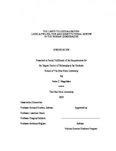
Figure 1.1 shows the various components of the GeForce GTX 280 and their logical organization. From the perspective of GPGPU, the GPU can be viewed as a many-core processor containing an array of Streaming Multiprocessors (SMs), each of which consists of 8 Scalar Processors (SPs), two transcendental function units, a multi-threaded instruction unit and fast, on-chip shared memory and a register-file. Each SP is also associated with off-chip local memory, which is mostly used for register spills and storing automatic arrays. In addition to these, each GPU device also contains large, slow, off-chip device memory. The number of SMs per device and the sizes of the various memories and the register file vary by device. 2

SP 0 IU

SP 1

SHARED MEMORY

SP 4

SP 5

SM 0

...

SP 0

SP 1

IU

SP 2

SP 5

SP 0 IU

SP 6

SP 4

SP 7

SP 2

SP 3

SP 0 IU

SP 6

SP 4

SM 7

SP 5

SP 2

SP 3

REGISTERS

SP 6

SP 7

SP 2

SP 3

... SP 1

SHARED MEMORY

REGISTERS

SP 7

SP 1

SHARED MEMORY

REGISTERS

SM 8

SHARED MEMORY

SP 4

SP 3

SP 5

REGISTERS

SP 6

SP 7

SM 15 DEVICE MEMORY

Figure 1.1: GPU Architecture

Table 1.1 summarizes the characteristics of the various kinds of GPU memory available on the GeForce GTX 280. There are two additional types of global memory: texture memory and constant memory, but we will not be making the distinction for the remainder of this discussion. Note that the latency of accessing global memory is orders of magnitude higher than accessing shared memory or the register file. Tolerating the high latency of global memory accesses is very important because data elements have to be moved from host (CPU) memory to the device’s global memory before it can be operated upon by the device. Similarly, the processed data elements need to be stored back in global memory for copying back to host memory. The task of effectively hiding the

3

Table 1.1: Characteristics of GeForce GTX 280 memory Memory Type On-chip or Access Size Off-chip? Latency Global Off-chip 400-600 cycles 1GB Local Off-chip 400-600 cycles Up to size of global Register On-chip No additional cycles 16K Shared On-chip Register latency 16KB

global memory access latency and managing the memory hierarchy is very crucial for obtaining maximal performance from the GPU. Each SM manages the creation, execution, synchronization and destruction of concurrent threads in hardware, with zero scheduling overhead, and this is one of the key factors in achieving very high execution throughput. Each parallel thread is mapped to an SP for execution, and each thread maintains it’s own register state. All the SPs in an SM execute their threads in lock-step, according to the order of instructions issued by the per-SM instruction unit. The SM creates and manages threads in groups of 32, and each such group is called a warp. A warp is the smallest unit of scheduling within each SM. The GPU achieves efficiency by splitting it’s work-load into multiple warps and multiplexing many warps onto the same SM. When a warp that is scheduled attempts to execute an instruction whose operands are not ready (due to an incomplete memory load, for example), the SM switches context to another warp that is ready to execute, thereby hiding the latency of slow operations such as memory loads.

4

1.1.2

CUDA Programming Model

NVIDIA’s Compute Unified Device Architecture (CUDA) is a programming model and hardware/software environment for GPGPU, which consists of the following components: • An extension to the C programming language that allows programmers to define GPGPU functions called kernels which are executed by multiple threads on the GPU. Commonly, a CUDA program is comprised of a single CUDA kernel, so the terms kernel and programs are used interchangeably for the remainder of this discussion. • A compiler and related tools for translating CUDA source code to GPU devicespecific binary • A software stack consisting of GPGPU application libraries, CUDA runtime libraries and CUDA device driver • A CUDA enabled GPU device The CUDA programming language provides a means for programmers to express a problem that exhibits significant data-parallelism as a CUDA kernel. A CUDA kernel is a function that is executed in Single Program Multiple Data (SPMD) on a large set of data elements. An example of a CUDA kernel for performing matrix-matrix multiplication is shown in Figure 1.2 The CUDA programming model organizes threads into a three-level hierarchy as shown in Figure 1.3. At the highest level of the hierarchy is the grid. A grid is a 2D array of thread blocks, and thread blocks are in turn, 3D arrays of threads. The GPU 5

__global__ void _deviceMul(float *A, float *B, float *C, unsigned size) { unsigned tx = threadIdx.x, ty = threadIdx.y, bx = blockIdx.x, by = blockIdx.y; /* The index is obtained by linearizing the 2D array */ unsigned vbDist = vBlockDist(by); unsigned vtDist = ty * gridDim.x * blockDim.x; unsigned hbDist = bx * blockDim.x; unsigned htDist = tx; unsigned index = vbDist + vtDist + hbDist + htDist; unsigned aStart = vbDist, aEnd = aStart + (gridDim.x * blockDim.x), aStep = blockDim.x; unsigned bStart = hbDist, bStep = gridDim.x * blockDim.x * blockDim.y; float Ctemp= 0.0; for (unsigned a = aStart, b = bStart; a < aEnd; a += aStep, b += bStep) { /* Copy to shared memory */ __shared__ float As[blockSize][blockSize], Bs[blockSize][blockSize]; As[ty][tx] = A[a + ty * gridDim.x * blockDim.x + tx]; Bs[ty][tx] = B[b + ty * gridDim.x * blockDim.x + tx]; __syncthreads(); /* Perform multiplication */ for (unsigned i = 0; i < blockDim.x; ++i) { Ctemp += As[ty][i] * Bs[i][tx]; } __syncthreads(); } /* Store computed result back to global mem */ C[index] = Ctemp; }

Figure 1.2: Matrix-matrix multiplication using CUDA

hardware scheduler maps one or more thread blocks onto each SM and the threads in a thread block are split into warps as described in Section 1.1.1 and scheduled onto the SPs. Threads belonging to the same thread block can co-operate with each other, by sharing the low-latency, on-chip shared memory and also through barrier synchronization. Synchronization across thread-blocks is not directly supported by the programming model. The size of the grid and the thread-blocks are determined by the programmer, according to the size of the problem being solved and communicated to the driver at kernel launch time. Each thread-block in a grid has it’s own unique identifier and each thread has a unique identifier within a block. Using a combination of block-id and

6

DEVICE GRID 0 Thread Block (0, 0)

Thread Block (1, 0)

Thread Block (2, 0)

Thread Block (3, 0)

Thread Block (0, 1)

Thread Block (1, 1)

Thread Block (2, 1)

Thread Block (3, 1)

Thread Block (0, 2)

Thread Block (1, 2)

Thread Block (2, 2)

Thread Block (3, 2)

Thread Block (0, 3)

Thread Block (1, 3)

Thread Block (2, 3)

Thread Block (3, 3)

THREAD BLOCK (3, 0) Thread (0, (0,0) 0)

Thread (1, 0)

Thread (2, 0)

Thread (3, 0)

Thread (0, 1)

Thread (1, 1)

Thread (2, 1)

Thread (3, 1)

Thread (0, 2)

Thread (1, 2)

Thread (2, 2)

Thread (3, 2)

Thread (0, 3)

Thread (1, 3)

Thread (2, 3)

Thread (3, 3)

...

...

Figure 1.3: Hierarchy of threads in the CUDA programming model

thread-id, it is possible to distinguish each individual thread running on the entire device. Only a single grid of thread blocks can be launched on the GPU at once, and the hardware limits on the number of thread blocks and threads vary across different GPU architectures and are discussed in detail, in later sections. It is important to note that two key resources of the SM, namely the shared memory and the register file, are shared by the thread-blocks that are concurrently active on the SM. For example, if each SM has 16KB of shared memory and each thread-block requires 8KB of shared memory, then no more than 2 thread blocks can be concurrently scheduled on the SM.

7

1.2

Compiler Optimizations and Loop Unrolling

Compilers translate program source code into target-specific binary code, while automatically performing deep analyses and optimizations of the source code along the way. Since compilers have an intimate knowledge of the underlying hardware, compiler optimizations play a key role in improving the performance of user programs. One such compiler optimization that has been researched and implemented in compilers for many years now is Loop Unrolling. Loop Unrolling is a technique in which the body of a suitable loop is replaced with multiple copies of itself, and the control logic of the loop is updated accordingly. Also, if necessary, a remainder loop is added at the end of the unrolled loop to handle cases where the loop trip count is not exactly divisible by the unroll factor. Figure 1.4 demonstrates how simple loop is unrolled by a factor of 4. The primary benefits gained from loop unrolling are: • Reduced dynamic instruction count, due to fewer number of compare and branch operations for the same amount of work done • Better scheduling opportunities due to the availability of additional independent instructions - the compiler’s scheduler can use these instructions for improving Instruction Level Parallelism (ILP) and hiding pipeline and memory access latencies • Opportunities for exploiting register and memory hierarchy locality when outer loops are unrolled and inner loops are fused (unroll-and-jam transformation) However, if loops are unrolled too aggressively, the benefits of unrolling can be undone and performance may degrade due to the following reasons: 8

/* Before unrolling */ for (i = 0; i < N; ++i) { c[i] = a[i] + b[i]; }

/* After unrolling */ for (i = 0; i < N - (4 - 1); i += 4) { c[i] = a[i] + b[i]; c[i+1] = a[i+1] + b[i+1]; c[i+2] = a[i+2] + b[i+2]; c[i+3] = a[i+3] + b[i+3]; } /* Remainder loop */ for (; i < N; ++i) { c[i] = a[i] + b[i]; }

Figure 1.4: Example of unrolling a simple loop 4 times

• Aggressive unrolling and scheduling can lead to increase in register pressure within the body of the loop. For CPU based programs, this could result in spilling of registers to memory, which could slow down the program. • If the loop is unrolled by a very large amount, the size of the loop body could overflow the instruction cache, leading to cache misses and hence, reduced performance.

1.3

Problem Statement

The effects of loop unrolling for CPU-based programs are well understood, and different strategies for efficiently choosing the optimal unroll factor at compile time

9

have been suggested [23, 12, 11, 13] and speedups of nearly 2X have been achieved under optimal unrolling. However, these results have not carried over to GPGPU programming. The vast differences in architecture and programming models between GPGPU and CPU based programming necessitates a new look at the impact of loop unrolling on the performance of GPGPU programs. Research in the area of GPGPU optimizations has established that loop unrolling is beneficial in many cases [9, 16, 21], but there has not been much success in finding compile-time techniques to determine optimal loop unroll factors. Loop unrolling for GPGPU has been looked at, in [9, 16], but these works rely on performing an empirical search of the optimization space, which can be very expensive and sensitive to program inputs. It is therefore very desirable to develop a compile-time technique for determining optimal loop unroll factors for GPGPU programs. In this thesis, we attempt to answer the following questions: 1. How can we accurately characterize the impact of loop unrolling on GPGPU programs? 2. Using the characterization, how can we design a system that predicts whether unrolling is beneficial for loops chosen by the user, and if so, what the optimal unroll factors are? 3. How can we minimize the number of unroll configurations evaluated while determining the optimal unroll factor?

10

1.4

Organization of Thesis

The rest of this thesis is organized as follows: In Chapter 2, we look at the compilation model for CUDA programs and discuss about the various factors that influence loop unrolling for GPGPU programs. We also present experimental evaluations to demonstrate the effect of unrolling on the corresponding factors. In Chapter 3, we present the detailed design of a system for predicting the optimal unroll factors for loops chosen by the user. We also describe the algorithms and formulas that guide the prediction system. We then present detailed experimental results that demonstrate the ability of the system to predict the optimal unroll factors, along with search space pruning. Finally, in Chapter 4, we summarize the contributions of our work and describe the direction of future work in this area.

11

CHAPTER 2

LOOP UNROLLING FOR GPGPU PROGRAMS

In this chapter, we look at the various factors that influence loop unrolling for GPGPU programs and their complex interplay, and try to understand why a significantly new approach for analyzing and selecting optimal unroll factors is necessary.

2.1

Background

In Section 1.1.1 we looked at the architecture of the GPU from the perspective of GPGPU, and understood how the architecture and programming model are different from CPU architectures and programming models. Now, we take a closer look at the various resources available on a GPU, and their constraints and limitations. We then examine how these resource constraints can influence compiler optimizations such as loop unrolling. Table 2.1 lists some of the important resources on the GTX 280, their sizes and their constraints. Typically, the size of resources such as the number of threads per block, the block dimensions and grid dimensions present a challenge to the programmer, who has to make the best use of these resources to solve the problem at hand. However, the most important resource from the perspective of the compiler is the register-file. Since the entire register-file on an SM is shared among all the threads 12

Table 2.1: GTX 280 resources, their sizes and constraints Resource Size Constraint Total global memory 1GB None Total shared memory per SM 16KB Shared by all concurrent blocks Total number of register per SM 16K Shared by all concurrent threads Warp size 32 None Max threads per block 512 None Max dimensions of a block 512, 512, 64 None Max dimensions of a grid 64K, 64K, 1 None

concurrently executing, if a compiler optimization increases the register usage per threads, then the number of threads that can execute concurrently reduces. Therefore, this trade-off needs to be considered by all optimizations that may increase the per-thread register usage. Since loop unrolling is one such optimization, we need to examine the effects of loop unrolling for GPGPU programs in the context of these resource constraints, and try to characterize the impact of unrolling on GPGPU programs, before we make an attempt to analyze if a given GPGPU loop will benefit from loop unrolling, and if so, what the optimal unroll factor is.

2.2

Factors Influencing Loop Unrolling For GPGPU Programs

We saw in Section 1.2 that loop unrolling is a compiler optimization that could possibly increase the speed of execution of loops in CPU-based programs, at the cost of increased register usage and increased code size. Even in the case of loops in GPGPU programs, unrolling produces the same effect of possibly reduced instruction counts,

13

increased opportunities for scheduling and register tiling, with the same pitfalls of increased register usage and code size. However, the differences in architecture and programming models, and the presence of resource constraints as described in Table 2.1 imply that the analytical models developed for selecting optimal loop unroll factors on CPU-based loops cannot be directly extended to GPGPU loops. In the following sections, we look at the impact of loop unrolling on loops in GPGPU programs.

2.2.1

Instruction Count

One of the most obvious benefits of unrolling loops is the reduction of instruction count. The primary source of reduction in instruction count is the fewer number of compare and branch instructions necessary for performing the same amount of computation as compared with the original version. Instruction count may also reduce because of the better instruction selection, scheduling and optimizing opportunities that result from unrolling. The reduction in instruction count directly improves the performance of the loop, and loops in GPGPU programs benefit from this optimization the same way as loops in CPU programs.

2.2.2

ILP and GPU Occupancy

Loop unrolling, in general, provides better instruction scheduling opportunities to the compiler because it increases the number of available independent operations within the body of the loop. Increased independent operations within the loop body could lead to increased Instruction Level Parallelism (ILP) and the compiler could use the additional independent operations to hide latencies of pipelines and memory access. 14

For CPU based programs, exposing Instruction Level Parallelism (ILP) in code is one of the key approaches for hiding pipeline and memory access latency. However, aggressive scheduling for ILP by the compiler could lead to increased register pressure within the loop body which can lead to register spills, and thereby reduce performance. Therefore, it is necessary to balance the boost in ILP resulting from loop-unrolling, with the register spills, and ensure that there is no performance degradation due to unrolling. Previous work, such as [23], manages this trade-off effectively and selects optimal unroll factors for CPU-based loops. For loops in GPGPU programs, ILP plays a significant role in hiding pipeline and global memory access latencies, but there is another key factor that is just as important, if not more, for hiding latencies: GPU occupancy. The GPU tolerates latencies by multiplexing a large number of warps onto each SM, up to the limit allowed by resource constraints, and when a warp that is executing encounters a high latency operation, the scheduler switches execution to another warp that is ready for execution. By the time all warps are cycled and the first warp that was switched out is switched back in, it is likely that the high latency operation would have completed. Therefore, GPUs rely on a combination of ILP and occupancy to tolerate high latencies. Due to this complex interplay of ILP and occupancy inside a GPU, estimating the benefit from increased ILP on the overall performance of the program is hard. This is because, increase in register usage, which mostly comes with increase in ILP reduces GPU occupancy since the register file is a resource shared by all active threads. Therefore, any model for estimating the benefit of loop unrolling must accurately model the trade-off between increased ILP and decreased occupancy. 15

We attempt to characterize this trade-off in Section 3.2.5.

2.2.3

Instruction Cache Size

An obvious result of loop unrolling is the increase in size of the loop body. This result does not have a negative impact on the performance of the loop body as long as the entire loop body fits into the instruction cache or I-cache of the processor. When the size of the loop body exceeds that of the I-cache, then cache misses occur whenever a portion of the loop body that is not in the cache is to be executed. These cache misses could reduce the performance of the program and it could even undo some of the benefits gained by reduced instruction count and increased ILP. The effect of the I-cache on loop unrolling is the same for CPU based programs, as well as for GPGPU programs. Past work in the area of loop unrolling for CPU based programs, such as [23], take into account the effect of the I-cache and there have been efforts such as [27] to automatically measure the size of CPU I-caches so that it can be useful for unrolling compilers, among others. The size of the I-caches on NVIDIA GPUs are not documented by NVIDIA and there are no known techniques for automatic measurement of I-cache capacities on GPUs. Therefore, we decided to run experiments similar to the experiments described in [27], but designed to run on a GPU instead, in order to determine the size of the I-cache on the GPU on which our experiments were running. Figure 2.1 shows the CUDA kernel we’ve implemented to help estimate the size of the I-cache on the GPU. The code primarily consists of a compute-intensive loop with a very large trip count. The loop is successively unrolled by multiples of two

16

until the body of the loop overflows the I-cache. When the overflow is detected, the size of the loop body is computed, and we have an upper bound for the size of the I-cache. Changing the number of operations in the body of the original loop allows us to experiment with different sizes of the loop body, so that the upper-bound on the I-cache size can be tightened.

__global__ void icache_kernel(unsigned long u, volatile unsigned long *res) { volatile register unsigned long v = u; unsigned p0 = v, p1 = v, p2 = v, p3 = v, p4 = v, p5 = v, p6 = v; unsigned i = 0; /* Total #iters = 1048576; expected result: 6291462 */ for (i = 0; i < 1048576; ++i) { p1 += p0; p2 += p0; p3 += p0; p4 += p0; p5 += p0; p6 += p0; } /*@ end @*/ v = p1 + p2 + p3 + p4 + p5 + p6; *res = v; }

Figure 2.1: Estimating the size of the I-cache on the GTX 280

The main requirement of this code is to isolate the effect of the I-cache from among other factors such as pipeline depths and memory access latencies, so that there is an observable decrease in the performance of the kernel, when the loop body overflows the I-cache. The code uses the following techniques to achieve this requirement:

17

• By having enough instructions in the loop body between a write to a register and the next read from the same register. This ensures that the latency of the arithmetic pipeline is fully covered, and there are no RAW hazards. The latency of the arithmetic pipeline in the GTX 280 is 24 cycles, so having 6 independent instructions in the loop body takes care of this requirement, because each arithmetic instruction takes 4 cycles to issue. • By having all operands in registers and ensuring that there are no memory loads or stores in the body of the loop. This eliminates the effect of memory latencies from the performance of the loop. • By ensuring that there is only warp per thread block and only one thread block per SM in the kernel launch configuration. This ensures that there are no additional warps to hide the latency of an I-cache miss when it occurs, and therefore a performance drop is guaranteed when an I-cache miss occurs. The results of running this experiment are summarized in Figure 2.2. From the results, we can observe that there is always a drop in performance when the size of the loop body crosses the threshold of 32KB. Therefore, we conclude that the size of the I-cache on the GTX 280 is 32KB in size and use this information for analyzing optimality of unroll factors.

2.3

Summary

In this section we have presented the various factors that influence unrolling of loops in GPGPU programs. We have also discussed how these factors differ from similar factors on CPU based platforms and why existing work in the areas of loop

18

200 6 instrs per iter 8 instrs per iter 9 instrs per iter 12 instrs per iter

180

Run-time (ms)

160 140 120 100 80 60

0

10

20

30

40 50 60 Loop body size

70

80

90

100

Figure 2.2: Results of I-cache estimation experiments

unrolling for CPU based programs cannot be directly extended to GPGPU programming. We have discussed in detail, how the trade-off between ILP and GPU occupancy is very crucial for analyzing the effect of loop unrolling. Finally, we have presented an experimental technique to measure the capacity of the I-cache on GPU devices, and the results of using this technique.

19

CHAPTER 3

SELECTION OF OPTIMAL UNROLL FACTORS FOR LOOPS IN GPGPU PROGRAMS

This chapter describes the design and detailed working of the system that performs the selection of optimal loop unroll factors for loops in CUDA GPGPU programs. This chapter also presents detailed experimental results of using this system for selecting optimal unroll factors.

3.1

Design Overview

In this section, we look at the high-level design of the framework for selecting optimal loop unroll factors for user-specified loops in CUDA programs. The framework is centered around two components: the PTX Analyzer and the Unrolling Driver, which make use of a chain of other tools to help analyze the given kernel. Figure 3.1 provides a high-level overview of the design of the framework. The analysis framework requires that the loops/loop-nests selected by the user for unrolling have no conditional control-flow within their bodies. This is because the analysis is purely static, while analyzing loops with conditional control-flow in their bodies would require some dynamic analysis, such as profiling, in order to correctly 20

model the control-flow. It must be noted that this is not an overly-constraining requirement because branching within loop bodies could produce warp divergence, leading to reduced performance and this constraint ensures that most GPGPU programmers try to avoid or minimize conditional control-flow within loop bodies. In addition, the NVIDIA GPU ISA allows predicated execution of instructions, which can be used to achieve limited control flow within loop bodies, without significant performance loss, and loops with such predicated control flow are accepted by the analyzer.

Annotated CUDA source

ORIO

Start/Stop, New Unroll Factors

Unrolled CUDA source

NVCC

PTX ANALYZER Warp Count, Iteration Count, Unroll Factor

Compiled CUBIN

DECUDA

Estimated execution cycles, stall cycles

Disassembled PTX

OCF

OCF and Occupancy Info

UNROLLING DRIVER

Figure 3.1: Overview of the optimal unroll factor estimation framework

The components of the framework are:

21

1. ORIO: Input: Annotated CUDA source code with loop identifiers and unroll factors. Output: CUDA source code with loops unrolled by specified amount. Description: ORIO [14] is a source-to-source transformation tool that performs semi-automatic unrolling of loops. ORIO expects the user to annotate the source code indicating the loop to be unrolled and the unroll factor, after which ORIO unrolls the specified loops by the specified amount, ensuring legality of loop bounds in the unrolled code and adding remainder loops where necessary. In this framework, the user is expected to annotate the source code to identify the loops that need to be analyzed. The driver is responsible for inserting appropriate unroll factors for analysis. ORIO consumes CUDA source code annotated with loop identifiers and unroll factors and produces CUDA source with the loops unrolled appropriately.

2. NVCC: Input: CUDA source code with unrolled loops Output: GPU executable code (CUBIN) Description: NVCC is NVIDIA’s compiler driver that is responsible for translating CUDA source code to GPU device specific ISA. Details about NVCC and the compilation flow in NVCC can be found in [3]. We chose to explicitly compile different versions of the kernel with different unroll configurations using NVCC, instead of basing our analysis entirely on a theoretical model because the idiosyncrasies of the compiler’s code-generation 22

and register allocation cannot always be modeled accurately from outside the compiler - NVIDIA’s CUDA compiler back-end is NVIDIA proprietary, and we do not have enough insight into the workings of the compiler. Some of the experimental results in Section 3.3 corroborate this choice.

3. DECUDA: Input: NVIDIA CUBIN files Input: Disassembly of the CUBIN files in PTX format. Description: DECUDA [1] is a reverse-engineered disassembler for NVIDIA CUBIN files. The details of the CUBIN file format are not disclosed by NVIDIA, so it is virtually impossible to analyze the transformations and optimizations performed by NVIDIA’s proprietary compiler and their impact on the program’s performance. However, DECUDA disassembles compiled CUDA kernels in the CUBIN file into PTX format, which is documented and therefore, analyzable.

It is important to note that the PTX output from DECUDA is not identical to the PTX output generated by NVCC under the -ptx flag. The PTX generated by NVCC is an intermediate representation that has not yet been processed by the target-specific NVIDIA compiler back-end, ptxas, which performs important transformations and optimizations, such as register allocation and instruction scheduling. Since these optimizations have a very significant impact on the performance of the program, analyzing the PTX generated by NVCC is not very beneficial. However, DECUDA recreates PTX from after the optimizations have been performed by ptxas, which makes the DECUDA output equivalent to the 23

actual code that will be executed on the device. Analyzing this code is likely to give us greater insight into the behavior of the program and increase the accuracy of analysis and estimation.

4. OCF: Input: Disassembled PTX of a CUDA kernel from DECUDA Output: Various details related to the occupancy of the GPU Description: The Occupancy Constraining Factor (OCF) component gathers information about the resource usage by the kernel and computes the distribution of thread blocks to each SM and the maximum number of warps that can be concurrently active on each SM based on the device-specific resource constraints and usage. Details about the working of OCF can be found in Section 3.2.1.

5. Driver: Input: GPU Occupancy information from OCF and estimate of cycles spent in execution of loops under consideration, from PTX Analyzer Output: Selection of optimal unroll factors for the given CUDA kernel; Decisions of which unroll factors to evaluate and when to stop evaluation. Description: The Driver is the central controller of the framework. It is responsible for collecting all the information required for guiding the search for optimal unroll factors from the various entities like OCF and PTX Analyzer and efficiently performing the search. The Driver controls the execution of the compilation and disassembly tool-chain based on the inputs from OCF and PTX 24

Analyzer. Details about the working of the Driver are provided in Section 3.2.2.

6. PTX Analyzer: Input: Disassembled PTX of a CUDA kernel from DECUDA and information about active warp count, iteration count and unroll factors from Driver Output: Estimate of the number of cycles spent in executing the given CUDA kernel; estimate of the number of stall cycles. Description: The PTX Analyzer is a static program analysis tool that consumes the disassembled PTX representation of a CUDA kernel and rebuilds the Control Flow Graph (CFG) [7] and detects loops in the kernel. Using information about the active warp count, iteration count and loop unroll factors provided by the Driver, it estimates the number of cycles spent in the bodies of loops under consideration. It also estimates the number of GPU stall cycles incurred during execution of the kernel. The Driver passes loops unrolled with various unroll factors to the analyzer, and uses the estimated cycle counts to select the optimal unroll factor. More details about the PTX Analyzer are provided in Sections 3.2.3 and 3.2.4.

3.2

Detailed Design

In this section, we describe, in detail, the implementation of the key components of the framework for selecting optimal loop factors for user-specified loops in CUDA programs.

25

3.2.1

Occupancy Constraining Factor

The OCF component is responsible for reading the details of resource usage by the current CUDA kernel and computing the occupancy constraining factor and the maximum occupancy of each SM on the device for use by the Driver. Specifically, OCF consumes the following inputs: • GPU resource consumption by the given kernel: Per-thread register usage and per-block shared memory usage. • Resource limits of the GPU device being targeted, such as the limits presented in Section 2.2 • Kernel launch configuration: Number of thread blocks per grid and number of threads per thread block. Based on these inputs, OCF computes the maximum occupancy of each SM on the device, i.e the maximum number of thread blocks/warps that can be scheduled concurrently on each SM on the device. This information is used by the Driver to compute the number of iterations of thread block execution to be performed by each SM, which is then used to accurately estimate the number of execution cycles, by the PTX Analyzer. Equations 3.1 through 3.6 describe the computations performed by OCF. The maximum occupancy for each SM in the device, OCCmax , is given by: OCCmax = min(OCCreg , OCCsmem , OCCthreads , OCCblocks , OCCwarps )

(3.1)

where OCCreg , OCCsmem , OCCthreads , OCCblocks , OCCwarps represent the maximum occupancy for each SM due to the constraints on register usage, shared memory usage, thread count, thread block count and warp count respectively. These values are 26

computed in isolation, without the effects of other resource constraints and are given by the following equations.

OCCreg = bRegsSM /(Regsthread × T hreadsblock )c

(3.2)

where RegsSM is the number of registers available per SM, Regsthread and T hreadsblock represent the number of registers per thread and number of threads per block for the given kernel.

OCCsmem = bSmemSM /Smemblock c

(3.3)

where SmemSM is the amount of shared memory available per SM and Smemblock is the amount of shared memory consumed by each thread block in the given kernel.

OCCthreads = bT hreadsSM /T hreadsblock c

(3.4)

where T hreadsSM is the maximum number of threads allowed per SM by the hardware and T hreadsblock is the number of threads per block in the given kernel’s specification.

OCCblocks = BlocksSM

(3.5)

where BlocksSM is the maximum number of thread blocks per SM allowed by the hardware.

OCCwarps = bW arpsSM /W arpsblock c

(3.6)

where W arpsSM is the hardware limit on the maximum number of warps per SM and W arpsblock is the number of warps per block in the given kernel. W arpsblock is the 27

same as T hreadsblock /32.

The details of the hardware limits on the various resources for GTX 280 are discussed in Section 2.1.

3.2.2

Driver

The Driver is central controlling component that drives the other components in the framework, and uses the information produced by them to efficiently evaluate different unroll factors for user-specified loops in the given CUDA kernel. The Driver executes in a loop in which it systematically increases the unroll factors of the specified loops, starting from 1 and annotates the user-annotated CUDA source with the current unroll factor(s). It then invokes the tool chain containing ORIO, NVCC, DECUDA and OCF on the annotated source. At the end of the tool chain execution, the OCF component computes the maximum occupancy of each SM in the device, based on the resource consumption by the kernel, with unrolled loops. Using this occupancy information, the Driver invokes the PTX Analyzer to analyze the disassembled PTX and estimate the number of execution cycles spent by the kernel. The Driver maintains a table of estimated execution cycles corresponding to the various unroll factors and updates the table with the results of analysis from PTX Analyzer for each new unroll configuration. The driver terminates the evaluation of unroll factors when one of the following events occur: • The unroll factors reach a user-specified upper limit. If the user is aware of the maximum amount by which the loops can be unrolled, the Driver makes use of 28

this information. If this information is not available, the Driver uses it’s own internal limit to stop the search. • When the resource usage, specifically the register usage per thread, increases to an extent where not even a single thread block can be scheduled on an SM. The CUDA runtime will not allow a kernel with an occupancy of less than 1 thread-block per SM to be launched. • When the size of the outermost loop being unrolled reaches or exceeds the size of the SM’s instruction cache, as described in Section 2.2.3. In practice, we observed very few cases in which the evaluation had to be terminated due to this event - the two earlier causes were more common. At the end of the evaluation the Driver selects the unroll configuration with the least estimated execution cycles as the optimal unroll factor from it’s table of results. If however, the Driver finds that the kernels with unrolled loops perform worse than the original version with no unrolling, it reports that unrolling is not beneficial for the given kernel. We now look at how the Driver uses the occupancy information generated by OCF to query the PTX Analyzer for accurate estimates of executed cycles. The Driver receives the value of maximum occupancy, OCCmax from OCF and the total number of blocks to scheduled on the device, Blockstotal from the user and computes the following values:

BlocksSM = dBlockstotal /SMdevice e

(3.7)

where BlocksSM is the total number of blocks assigned to each SM for execution.

29

F ullItersSM = bBlocksSM /OCCmax c

(3.8)

where F ullItersSM is the number of full iterations, i.e. iterations for which each SM can execute with maximum occupancy OCCmax . Along similar lines, we also have:

P artialItersSM

( 1, if (BlocksSM mod OCCmax ) 6= 0 = 0, otherwise

(3.9)

where P artialItersSM gives the number of partial iterations, i.e iterations for which each SM can execute with occupancy less than OCCmax . Basically, OCCpartial is the number of blocks that remain to be executed after all the full iterations have completed. This occupancy level, OCCpartial is computed as:

OCCpartial = BlocksSM − (F ullItersSM × OCCmax )

(3.10)

Using this information, the Driver computes the active warp count that is required by the PTX Analyzer for estimating the execution cycles.

Wf ull = OCCmax × W arpsblock

(3.11)

Wpartial = OCCpartial × W arpsblock

(3.12)

where, Wf ull is the number of active warps in each of the full iterations, Wpartial is the number of active warps for the duration of the partial iteration, if any, and W arpsblock is the number of warps per block, as described in Equation 3.6.

30

The Driver stores the current unroll configuration in a file that can be accessed by the PTX Analyzer for it’s analysis. Finally, the Driver uses uses the computed values of Wf ull , F ullItersSM , Wpartial and P artialItersSM along with the iteration count I to invoke the PTX Analyzer, get the estimated execution cycle counts for the various loops/loop nests in the CUDA kernel and compute the total execution cycles. Specifically, the computation of total execution cycles, Cyclestotal is performed in two steps, as shown below:

CyclesL = ((ComputeLoopCycles(L, Wf ull , I) × F ullItersSM ) +(ComputeLoopCycles(L, Wpartial , I) × P artialItersSM ))

(3.13)

X

(3.14)

Cyclestotal =

CyclesL

For all outer loops L

where ComputeLoopCycles is an invocation of the PTX Analyzer to estimate the number of cycles spent in the body of the given loop, with the given active warp count and iteration count. ComputeLoopCycles is described in detailed in Section 3.2.4. For every unroll configuration evaluated, the Driver stores the value of Cyclestotal along with unroll configuration. When all unroll configurations have been evaluated, the one for which Cyclestotal has the least value is chosen as the optimal unroll configuration. It is important to note that we do not attempt to estimate the actual number of cycles spent inside the body of L. Instead, we assume that the original version of every loop L has an iteration count I, which may not be exactly equal to or even close to the actual iteration count of L. As the body of L is unrolled and analyzed, 31

we divide I by U FL , the current unroll factor for L and use that as the iteration count for estimating the cycles spent in the body of the unrolled loop. This gives us an estimate of the relative performance of the loop body under different unroll factors, instead of an estimate of actual performance. We use the relative differences in estimated performance to select the optimal unroll factor.

3.2.3

PTX Analyzer

The PTX Analyzer is the core analysis component of the framework. It reads the disassembled PTX file generated by DECUDA, and discovers many useful attributes of the CUDA kernel represented by the PTX file and is therefore a very useful tool for understanding the structure, behavior, and performance characteristics of the compiled CUDA kernel. Among the interesting attributes gathered by the PTX Analyzer, the important ones are: • Number of instructions in the kernel and categorization of their types. • The ratio of arithmetic operations to memory operations. • Control Flow Graph (CFG) of the kernel, which can be printed to file for visual inspection. • Number of loops in the kernel, their nesting levels, the number and type of instructions in their bodies and their ratios. • Estimate of number of cycles spent in executing each of the identified loops. Although we use the PTX Analyzer for only estimating the number of execution cycles in loop bodies in this thesis, the other options have been very useful for analyzing and understanding the behavior of many CUDA kernels.

32

Entry block

BB 0 (Instruction count: 11) set.eq.u32 $p0|$o127, s[0x0010], $r60 (A) mov.half.b32 $r9, s[0x0010] (S) mov.half.b32 $r0, s[0x0010] (S) mov.b32 $r1, s[0x0014] (S) @$p0.ne set.eq.u32 $p0|$o127, s[0x0014], $r60 (A) mov.half.b32 $r4, $r9 (A) mov.half.b32 $r5, $r9 (A) mov.half.b32 $r6, $r9 (A) mov.half.b32 $r7, $r9 (A) mov.b32 $r8, $r9 (A) @$p0.ne bra.label label2 (B)

BB 1 (Instruction count: 2) mov.b32 $r2, $r124 (A) mov.b32 $r3, $r124 (A)

BB 2 (Instruction count: 1) Loop Header (Nesting depth 0) label0: mov.b32 $r10, $r124 (A)

BB 3 (Instruction count: 9) Loop Header (Nesting depth 1) Loop Footer label1: add.b32 $r10, $r10, 0x00000001 (A) add.half.b32 $r6, s[0x0010], $r6 (A) add.half.b32 $r7, s[0x0010], $r7 (A) add.u32 $r8, s[0x0010], $r8 (A) set.ne.u32 $p0|$o127, $r10, c1[0x0000] (A) add.half.b32 $r9, s[0x0010], $r9 (A) add.half.b32 $r4, s[0x0010], $r4 (A) add.u32 $r5, s[0x0010], $r5 (A) @$p0.ne bra.label label1 (B)

BB 4 (Instruction count: 6) Loop Footer add.u32 $p0|$r2, $r2, c1[0x0004] (A) addc.u32 $r3, $r3, $r124 (A) set.eq.u32 $p0|$o127, $r3, $r1 (A) @$p0.ne set.lt.u32 $p0|$o127, $r2, $r0 (A) @$p0.eq set.lt.u32 $p0|$o127, $r3, $r1 (A) @$p0.ne bra.label label0 (B)

BB 5 (Instruction count: 8) label2: add.half.b32 $r2, $r6, $r7 (A) add.half.b32 $r1, $r4, $r5 (A) add.half.b32 $r0, $r8, $r9 (A) add.half.b32 $r1, $r1, $r2 (A) add.half.b32 $r2, $r0, $r1 (A) mov.half.b32 $r0, s[0x0018] (S) mov.b32 $r3, $r124 (A) mov.end.b64 g[$r0], $r2 (G)

Exit block

Figure 3.2: Sample CFG printed by PTX Analyzer 33

PTX Analyzer parses the PTX file output by DECUDA and using it’s knowledge of the PTX ISA, identifies and categorizes the instructions as arithmetic operations, branch operations (conditional/unconditional), memory loads/stores, synchronization operations and other miscellaneous operations. Further, it also distinguishes between the different kinds of memory being accessed (global, local, shared). Once the instructions are categorized, the analyzer uses standard techniques described in compiler literature such as [7], for identifying basic-blocks, and the flow of control between them, and constructing the CFG of the kernel. Figure 3.2 shows an example of the CFG of a simple CUDA kernel with one loop nest made of two loops that the PTX Analyzer has identified and printed. The analyzer has identified the different basic blocks in the kernel and the flow of control between them. For each basic-block, the number of instructions has been identified and printed, and along-side each instruction, it’s type A - arithmetic, B - branch, S - shared mem op, G - global mem op is printed. Also, the loops in the kernel have been identified and tagged with their nesting depths and header/footer blocks. By making use of the low-level details about the CUDA kernel provided by the PTX Analyzer, we propose a technique to estimate the number of execution cycles spent in the bodies of various loops in the kernel, using which the Driver can select the optimal loop unrolling configuration. The following section describes the technique for estimate execution cycles in loop bodies.

34

3.2.4

Estimating the Number of Cycles

In this section, we describe the technique used to estimate the number of cycles spent in executing the body of a given loop/loop nest L. This estimate is used by the Driver to select the optimal unroll configuration from among many configurations as described in Section 3.2.2. The key to estimating the number of execution cycles is to model the behavior of the CUDA scheduler, which is responsible for scheduling the thread blocks on to the SMs in the device, and for switching from one warp to another when the current warp encounters a blocking instruction. However, the behavior of the scheduler has not been disclosed by NVIDIA, but previous research [20] has indicated that a roundrobin scheduling can be used for modeling the behavior. We too use a model with round-robin scheduling of warps, i.e when the current warp is switched out because of executing an instruction whose operands are not ready, we assume all the remaining active warps are scheduled before returning to the first warp. Also, we assume a static, equal distribution of thread blocks to SMs. The procedure for estimating the total number of cycles spent in the body of a given loop, with a given active warp count and iteration count is described in Figures 3.3 through 3.4. The main routine in estimation is ComputeLoopCycles, and is implemented inside the PTX Analyzer. ComputeLoopCycles takes as input L, the CFG representation of a loop/loop-nest, W , the number of warps currently active on the SM and I, the assumed iteration count for all versions of loop L. The iteration count I is divided by U FL , the unroll factor for L so as to amortize the cycle counts by the unroll factor. The procedure then walks through the instructions in the body of the loop from top to bottom, accumulating cycles based on the type of 35

instruction seen, using the procedure ProcessInstr . If it detects an inner loop, it calls itself recursively and computes the cycle counts in the inner loop and updates the current cycle counter with counts from the inner loop as well. When the cycle counts for a single iteration of the complete loop body have been computed, they are multiplied by the iteration count which was previously amortized by the unroll-factor for the current loop, and returned to the Driver for further analysis. Since the loops accepted by the analyzer are free of conditional control-flow in the loop body, the only branches present in the loop body will be the back-edges from the loop-footer to the loop-header and the loop-exit branch, which makes the loop CFG traversal relatively straightforward. ComputeLoopCycles maintains two different counters: Cyclescurrent tracks the number of cycles incurred since the current warp was scheduled back after a warp switch (or from the beginning of execution before the first switch) while Cyclestotal tracks the total number of cycles spent across all warps since the beginning of execution. In addition, ComputeLoopCycles also creates a table T for tracking loads from global or local memory that whose operands have not yet been read. The procedure ProcessInstr described in Figure 3.4 is responsible for updating the counters and table based on the type of instruction encountered. ProcessInstr is called from ComputeLoopCycles whenever it encounters a new instruction in the loop body. ProcessInstr examines the current PTX instruction and updates the cycle counts with appropriate values assumed to be provided by the generic procedure GetCyclesForInstr . As long as no instructions that cause a warp switch are encountered, Cyclescurrent is updated with cycle count of the current instruction. When a load from global or local memory is seen, a new entry keyed on 36

ComputeLoopCycles: Estimate the number of cycles spent in the given loop body Input: CFG of input loop: L, Active warp count: W , Number of loop iterations: I Output: Estimated number of cycles spent in body of loop L 1. Cyclescurrent ← 0 Cyclestotal ← 0, T ← New table of pending loads, with keys as registers and values as cycle counts I ← I/U nrollF actorL 2. If L contains any blocking instruction, Then (a) Cyclescurrent ← ComputeFinalCycles(L) 3. For each basic-block B in L, from loop header to loop footer, Do (a) If B is the header of an inner-loop IL, Then Cyclestotal ← Cyclescurrent + (Cyclescurrent × W ) Cyclescurrent ← 0 Cyclestotal ← Cyclestotal +ComputeLoopCycles(IL, W, I) B ← successor block of loop footer of IL Go to line 3a (b) For each instruction Instr in B Do ProcessInstr(Instr, Cyclescurrent , Cyclestotal , W , T ) If Instr is the last blocking instruction in L, Then Break out of all surrounding loop nests Done Done 4. Cyclestotal ← Cyclestotal + (Cyclescurrent × W ) 5. Return Cyclestotal × I

Figure 3.3: Estimating number of cycles spent in a given loop

the destination register of the load is added to the table. Whenever the cycle counters are updated, the cycle counters corresponding to all the existing table entries are also updated. This is performed by the procedure UpdatePendingLoads. For each instruction examined, ProcessInstr checks if any of the source operands of the instruction is a destination of a pending load present in the table. If it is, and the number of cycles corresponding to the load are not sufficient to hide the latency

37

of the memory load, then a warp-switch is caused and the cycle counters are updated accordingly. Since this load is now complete, the corresponding entry is removed from the table. If loop L contains an instruction that could cause a warp-switch, then we need to compute, what are called final cycles. Calculation of final cycles is necessary to increase the accuracy of estimation of executed cycle counts and they specifically model the following scenario: Starting from iteration 2 through through iteration I − 1 of the loop L, when W arp0 , the first warp in the set of active warps executes InstrF W S , the first instruction in the loop body that causes a warp switch, the rest of the warps W arp1 through W arpW −1 are blocked at InstrLW S , the last instruction that caused a warp switch, in the previous iteration of the loop. Therefore, each warp in W arp1 through W arpW −1 now resumes execution at InstrLW S and continues till it reaches InstrF W S in it’s next loop iteration. Therefore, the number of instructions available to hide the latency of InstrF W S is not just W × (InstrF W S − Instr0 ), but instead is W × ((InstrF W S − Instr0 ) + (InstrN − InstrLW S )). The number of cycles accumulated in the range (InstrN − InstrLW S ) is called Final Cycles and is computed by the procedure ComputeFinalCycles, which is described in Figure 3.5. Strictly speaking, ComputeFinalCycles may not be completely accurate in some cases. It is likely to be accurate when InstrLW S is a barrier synchronization operation, but when InstrLW S is a global/local memory load, the actual warp switch will take place at a later instruction when the destination register of the load is read. Also, the memory load may have completed and may not result in a warp switch. But in practice, the technique used in ComputeFinalCycles is a good, conservative 38

ProcessInstr: Examine given PTX instruction and update cycle counts Input: Current PTX instruction: Instr, Cycles since last warp switch: Cyclescurrent , Total number of cycles: Cyclestotal , Active warp count: W , Table of pending loads: T Output: Updated cycle counts 1. For each source register SR in Instr, Do (a) If T contains an entry for SR, Then CyclesILP ← Value corresponding to SR in T If CyclesILP < Latencyglobal , Then Cycleswait ← M ax((Cyclescurrent × W ), Latencyglobal ) Cyclestotal ← Cyclestotal + Cycleswait Cyclescurrent ← 0 UpdatePendingLoads(T, Cycleswait ) T ← T − SR Done 2. Switch(Type of Instr) Global Mem Read: Local Mem Read: Cyclescurrent ← Cyclescurrent + 4 T ← T + new entry (Destination register of Instr, 4) UpdatePendingLoads(T , 4) Return Barrier Sync: Cyclescurrent ← Cyclescurrent + 4 Cyclestotal ← Cyclestotal + (Cyclescurrent × W ) UpdatePendingLoads(T , Cyclescurrent × W ) Cyclescurrent ← 0 Return All other types: Cyclescurrent ← Cyclescurrent + GetCyclesForInstr(Instr) UpdatePendingLoads(T , GetCyclesForInstr(Instr)) Return 3. Return

Figure 3.4: Determining cycle counts based on PTX instruction

approximation and will usually not result in over-computing final cycles, but could result in under-computing final cycles in some cases, which is unlikely to significantly 39

ComputeFinalCycles: Estimate the number of cycles spent between the last blocking instruction (global/local load, barrier sync) and the last instruction in the loop Input: CFG of input loop: L Output: Estimated number of cycles spent between the last blocking instruction and the last instruction in the body of loop L 1. Cyclesf inal ← 0 2. For each basic-block B in L, from loop footer to loop header, Do (a) For each instruction I in B, from last to first, Do If I is a blocking instruction, Then Return Cyclesf inal Else Cyclesf inal ← Cyclesf inal + GetCyclesForInstr(I) Done Done 3. Return Cyclesf inal

Figure 3.5: Estimating final cycles in a given loop

affect the relative performance differences required for predicting the optimal unroll factors.

3.2.5

Search Space Pruning

In this section, we discuss a technique which allows us to prune the search space for the optimal unroll configuration from among all possible unroll configurations.

Using estimated stall cycles to prune search space: The GPU does not attempt to reduce latencies of accessing global and local memories through the use of caches. Instead, it expects that sufficient ILP or a large number of active warps, or usually a combination of the two can be relied upon to tolerate such long latencies. Therefore, a reduction in ILP or reduction in the number of active warps, or 40

occupancy, can lead to situation where there are not enough instructions or warps to cover the latency of a pending global memory load (or less likely, the arithmetic pipeline). In such a situation, the GPU device stalls without performing any useful computation, and this situation is detrimental to performance. Since loop unrolling can boost ILP, but can increase register usage, which in turn can reduce occupancy, the effects of unrolling on stall cycles cannot be modeled directly. However, we can extend the cycle estimation framework discussed in previous sections to also estimate stall cycles for any given loop and unroll factor. Figure 3.6 describes an extension to the procedure ProcessInstr presented in Figure 3.4, which allows the PTX Analyzer to also track the number of stall cycles estimated to incur during the execution of the loop.

If ((Cyclescurrent × W ) < (Latencyglobal − CyclesILP )), Then Cyclesstall ← Cyclesstall + Latencyglobal − CyclesILP − (Cyclescurrent × W

Figure 3.6: Determining stall cycles in CUDA loops

Stall cycles, Cyclesstall are characterized as the number of cycles spent by the GPU device without executing any useful computation, waiting for a pending load to complete. When a warp that is executing issues an instruction whose source operands are the targets of a pending load, the scheduler switches to other warps that are ready to execute. However, after executing all these warps, when the first warp is scheduled again, if the load has not yet completed, then there are no more ready warps to switch to, and the GPU is forced to stall. When the product of the number of cycles since 41

the last warp switch Cyclescurrent and the active warp count W , is greater than the latency of the memory load, then there will be no stall cycles. This situation can be improved further, if CyclesILP , the number of cycles between the issue of the load and the use of the load, is high, since CyclesILP will reduce the latency of the global load accordingly.

Table 3.1: Stall cycle estimation for MonteCarlo kernel Unroll Register Max active blocks Factor Usage OCCmax 1 14 4 2 17 3 4 21 3 8 29 2 16 37 1 32 50 1

Max Active warps W arpsf ull 32 24 24 16 8 8

Estimated stall cycles 0 0 0 0 23808 27776

Measured Perf(ms) 169.81 140.74 130.87 127.22 154.09 167.12

The estimate of stall cycles can be used by the Driver to stop searching for optimal unroll factors when the total stall cycles incurred by the loop body increases as a result of reduction in GPU occupancy. When such an increase in stall cycles occurs, it is an indication that the occupancy levels have fallen below the minimum number of warps required to keep the GPU fully busy, or at least as busy as the original version of the loop. It is also an indication that no more boost in ILP is likely to overcome the reduction in performance due to drop in occupancy - that we have reached a point of diminishing returns and further search may be unnecessary. The results in Table 3.1 demonstrates the effect of computing stall cycles on the MonteCarlo simulation kernel on the GTX 280. We can observe that there are no 42

stall cycles estimated for the original version with no unrolling, but as successive unroll factors are compiled and evaluated, the ILP appears to increase, resulting in the increase of register usage and an increase in performance because there are still enough active warps to mask all the load latencies. However, when we reach an unroll factor of 16, the max occupancy drops to just 1 thread block or 8 warps per SM, and this results in GPU stalls and performance reduces significantly. This indicates that we have reached a point of diminishing returns, and the Driver could stop evaluating more unroll factors at this point. This result strengthens the theory that the Driver can use the increase in stall cycles with drop in occupancy as a factor for pruning the search space.

3.3

Experimental Results

In this section we present the results of using the system described in earlier sections to select optimal unroll factors for loops in CUDA applications and benchmarks. The experimental setup consisted of two systems running two different GPU devices: 1. A GTX 280 with 1GB of DRAM. The GTX 280 has 30 SMs clocked at 1.3 GHz and each SM has 8 processor cores, bringing the total count of processor cores on the device to 240. CUDA version 2.1 was used for compiling and running all CUDA kernels. Compilation level was -O3 for all experiments. The host CPU was an 8-core Intel Core i7 processor, clocked at 2.67 GHz with 6GB of RAM. A majority of the experiments were conducted on this system. 2. An 8800 GTX with 768 MB of DRAM. The 8800 GTX has 16 SMs clocked at 675 MHz and each SM had 8 processor cores, for a total of 128 processor 43

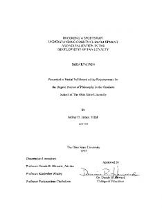
cores on the device. CUDA version 2.0 was used for compiling and running all kernels. The host CPU was a dual-core Intel Core2 Duo clocked at 2.13 GHz with 4GB of RAM. We have used CUDA kernels from the NVIDIA CUDA SDK and that Parboil Benchmark Suite from UIUC for demonstrating the effectiveness of the selection of optimal unroll factors. We first present a summary of the results of using the framework to select optimal unroll factors, and the speedup achieved from optimal unrolling. We then present detailed results and show the accuracy with which the framework estimates the relative differences in performance for various unroll configurations. Table 3.2 gives the summarized results and Figures 3.7 through 3.13 provide detailed results.

Table 3.2: Speedup achieved with optimal unrolling Benchmark

Run Time w/o Optimal Unroll Run Time w/ Speedup Unrolling (ms) Factors Chosen Unrolling (ms) 16K N-body (8800 GTX) 9712.51 256 8345.67 1.14 64K N-body (GTX 280) 23976.48 16 20188.27 1.16 M-M Multiply 1436.38 2, 16 787.6 1.45 Coulombic Potential 159.89 16 145.87 1.09 Monte-Carlo 169.81 8 127.22 1.25 BlackScholes (rlimit=16) 10.27 4 8.45 1.17 BlackScholes (no rlimit) 8.73 4 8.49 1.02

In the detailed results presented in Figures 3.7 through 3.13, subfigure (a) displays a graph of the number of cycles estimated by the framework for each unroll factor, subfigure (b) displays the measured performance of the kernel for each unroll 44

factor, allowing us to compare the estimation performance with actual measured performance. Subfigure (c) provides a relative comparison of estimated performance v/s measured performance of each unroll factor evaluated, relative to the estimated and measured performance, respectively, of the original program, with no unrolling. The BlackScholes computation CUDA kernel that is present in the NVIDIA CUDA SDK was configured by the original authors to use a maximum of 16 registers perthread in order to main high GPU occupancy. When the loop in the kernel was unrolled while keeping the register limit at 16, there was a 17 percent speedup. However, when the register limit was removed for compilation, the version without unrolling performed better than it’s counterpart with the register limit set. When the register limit was removed during unrolling, the register usage increased significantly when the the loop was unrolled 16 times or more. But by accurately computing the right occupancy factors, the Driver was able to correctly estimate the relative performance behavior of all the unroll versions, with and without register limit. Details can be found in Figures 3.13 and 3.12. Another interesting experiment was the N-Body simulation experiment. While selecting the optimal unroll factors for the kernel on the 8800 GTX with NVCC 2.0, we observed that the per-thread register usage did not increase significantly even up to unroll factors of 256 - in fact, performance of the loop steadily increased with every increasing unroll factor until it hit 256, which is an upper limit on the depth of unrolling. From Table 3.2, we can see that 256 is the optimal unroll factor for the NBody kernel on 8800 GTX. However, on the GTX 280, with NVCC 2.1, the per-thread register usage increased from 22 to 58 at unroll factor 32, reducing the occupancy by

45

35

9.6

Measured Running Time (sec)

9.8

34 33 32 31 30 29

1

2

4

8

16

32

64

9.4 9.2 9 8.8 8.6 8.4 8.2

128 256

1

2

Unroll Factors

4

8

16

32

64

128 256

Unroll Factors

(a) Predicted cycles

(b) Measured running time

18 Predicted Cycles Measured Time

16 Percent Reduction Relative To Base

Predicted Cycles (millions)

36

14 12 10 8 6 4 2 0

1

2

4

8

16 Unroll Factors

32

64

(c) Predicted v/s Measured

Figure 3.7: N-Body simulation of 16K bodies (8800 GTX)

46

128

256

20

23.5

Measured Running Time (sec)

24


20.5

19.5

23

22.5

19

18.5

22

21.5

18

17.5

21

20.5

17

1

2

4

8

16

32

20

64

1

2

4

Unroll Factors

8

16

32

64

Unroll Factors




Percent Reduction Relative To Base

14 12 10 8 6 4 2 0

1

2

4

8 Unroll Factors

16

32


Figure 3.8: N-Body simulation of 64K bodies (GTX 280)

47

64

110

1400

Measured Running Time (ms)

1500


120

1300

100

1200

90

1100

80

1000

70 60 50

900 800 700

1,1 1,2 1,4 1,8 1,16 2,16 4,16 8,16 16,16 32,16

1,1 1,2 1,4 1,8 1,16 2,16 4,16 8,16 16,16 32,16

Unroll Factors

Unroll Factors



100


Predicted Cycles Measured Time

80

60

40

20

0 1,1

1,2

1,4

1,8

1,16 2,16 Unroll Factors

4,16

8,16


Figure 3.9: M-M Multiply (4K X 4K) (GTX 280)

48

16,16

32,16

175 Measured Running Time (ms)

0.4 0.39


170

0.38

165

0.37

160

0.36

155

0.35

150

0.34 0.33

1

2

4

8

16

145

32

1

2

Unroll Factors

4

8

16

32

Unroll Factors





8 6 4 2 0 -2 -4 -6 -8

1

2

4

8

16

Unroll Factors


Figure 3.10: Coulombic Potential computation (GTX 280)

49

32

4.1 170

Measured Running Time (ms)

3.9

160

3.8 3.7

150

3.6

140

3.5 3.4

130

3.3 3.2

1

2

4

8

16

120

32

1

2

Unroll Factors

4

8

16

32

Unroll Factors






4

25

20

15

10

5

0

1

2

4

8 Unroll Factors


Figure 3.11: MonteCarlo computation (GTX 280)

50

16

32

12.5 Measured Running Time (ms)

2.1 2

12

1.8

11

10.5

1.7 1.6 1.5 1.4

1

2

4

8

16

32

10 9.5 9 8.5 8

64

1

2

4

Unroll Factors

8

16

32

64

Unroll Factors




0 Percent Reduction Relative To Base

Predicted Cycles

11.5

1.9

-5 -10 -15 -20 -25 -30 -35 -40 -45

1

2

4

8 Unroll Factors

16

32


Figure 3.12: Black-Scholes computation without register-limit (GTX 280)

51

64

12.5 Measured Running Time (ms)

1.7 Predicted Cycles (millions)

1.65

12

11.5

1.6

1.55

11

10.5

1.5

1.45 1.4

1.35

1

2

4

8

16

32

10 9.5 9 8.5 8

64

1

2

4

Unroll Factors

8

16

32

64

Unroll Factors





15 10 5 0 -5 -10 -15 -20

1

2

4

8 Unroll Factors

16

32


Figure 3.13: Black-Scholes computation with register-limit = 16 (GTX 280)

52

64

half and thereby decreasing performance! Once again, the Driver correctly selected the right unroll factors in each case.

3.4

Related Work

Loop Unrolling for CPU based programs have been studied for many decades now. Techniques for selecting optimal loop unroll factors for CPU based programs have been proposed in [23, 12, 11, 13]. However, as we have described in Section 2, the architectural differences, programming model requirements, and the different resource constraints of GPGPU dictate that the results from CPU based systems cannot be carried over directly to GPGPU systems. In GPGPU literature, it has been established that loop unrolling is a beneficial optimization for GPGPU programs [9, 16, 21] and attempts have been made to identify optimal loop unroll factors. [21] describes that loop unrolling can be used to reduce the dynamic instruction count in GPGPU programs and thereby increase performance, but does not describe a systematic way of analyzing unroll factors and selecting the most optimal among these. [9] and [16] both use empirical search for explicitly running various versions of the original program with different unroll factors, and using actual run times to guide the search further or choose the best unroll factor. However, empirical search has two drawbacks: the cost of having to run various versions of the program before picking the best one can be very high, especially if the program has a long running time. Also, empirical search, as with other dynamic analysis techniques is usually sensitive to program inputs. The results seen with a particular input may not be reproducible with a different input, requiring empirical search to be conducted for all possible program inputs, which may not be feasible.

53

[9] attempts to improve the quality of the search by using an analytical model to guide the search and [16] uses an adaptive compiler system to reduce the scope of empirical search. But neither of these techniques performs static, compile-time analysis, without having to run different versions of the program, and neither approach is completely input-agnostic. To the best of our knowledge, there is no other compile-time, static analysis technique that attempts to select optimal loop unroll factors for loops in GPGPU programs, like the technique described in this thesis. This technique performs analysis on the disassembled PTX code to estimate the number of cycles executed in the body of the given loop with an estimated trip count and produces a relative ordering of the performance benefits of the various unroll factors. The most optimal loop unroll factor is chosen from this relative ordering. Also, since our technique is static, it is input-agnostic.

3.5

Summary

In this chapter, we have described the detailed design and implementation of the framework that statically estimates execution cycle counts of a given CUDA loop, and uses that information to select the optimal unroll factor. We have also described in detail, the various tools that provide the required background information required for estimating cycle counts. In addition, we have described a strategy for pruning the search space of unroll factors, by estimating GPU stall cycles. Finally, we have provided detailed experimental results of using the above framework for selecting optimal loop unroll factors and shown speedups of up to nearly 50

54

CHAPTER 4

CONTRIBUTIONS AND FUTURE WORK

In this thesis, we have presented a detailed discussion of the factors influencing the unrolling of loops in GPGPU programs, specifically using NVIDIA’s CUDA as the target environment. We have also presented a technique for selecting optimal loop unroll factors for CUDA loops, by estimating the number of cycles executed by the various unrolled versions of the original loop. In addition, we have also extended the basic technique of estimating execution cycles to also compute GPU stall cycles and use that information to prune the search space of unroll factors. Finally, with detailed experimental results, we have demonstrated the effectiveness of the techniques described in this thesis and showed speedups of close to 50 The work described in this thesis has formed the basis for solving more interesting problems related to loop unrolling and other optimizations for GPGPU programs that we are looking at, such as the following: • How can the techniques described in this thesis be applied to other GPGPU programming models, such as OpenCL? • How can this technique be extended to support more complex transformations, such as unroll-and-jam of nested loops? 55

• Can the existing technique use profiling support or other means to handle loops with conditional control flow in the loop body?

56

BIBLIOGRAPHY

[1] DECUDA. http://www.cs.rug.nl/ wladimir/decuda/. [2] NVIDIA CUDA. http://www.nvidia.com/object/cuda home.html. [3] NVIDIA CUDA Documentation. http://www.nvidia.com/object/cuda develop.html. [4] NVIDIA GTX gtx 280 us.html.

280.

http://www.nvidia.com/object/product geforce

[5] NVIDIA TESLA Supercomputing. supercomputing.html.

http://www.nvidia.com/object/personal

[6] OpenCL. http://www.khronos.org/opencl/. [7] Alfred V. Aho, Ravi Sethi, and Jeffrey D. Ullman. Compilers: principles, techniques, and tools. Addison-Wesley Longman Publishing Co., Inc., Boston, MA, USA, 1986. [8] Sergio Barrachina, Maribel Castillo, Francisco D. Igual, Rafael Mayo, and Enrique S. Quintana-Ort´ı. Solving dense linear systems on graphics processors. In Euro-Par ’08: Proceedings of the 14th international Euro-Par conference on Parallel Processing, pages 739–748, Berlin, Heidelberg, 2008. Springer-Verlag. [9] Muthu Manikandan Baskaran, Uday Bondhugula, Sriram Krishnamoorthy, J. Ramanujam, Atanas Rountev, and P. Sadayappan. A compiler framework for optimization of affine loop nests for gpgpus. In ICS ’08: Proceedings of the 22nd annual international conference on Supercomputing, pages 225–234, New York, NY, USA, 2008. ACM. [10] Luc Buatois, Guillaume Caumon, and Bruno Levy. Concurrent number cruncher: a gpu implementation of a general sparse linear solver. Int. J. Parallel Emerg. Distrib. Syst., 24(3):205–223, 2009. [11] Steve Carr and Yiping Guan. Unroll-and-jam using uniformly generated sets. In MICRO 30: Proceedings of the 30th annual ACM/IEEE international symposium on Microarchitecture, pages 349–357, Washington, DC, USA, 1997. IEEE Computer Society. 57

[12] Steve Carr and Ken Kennedy. Improving the ratio of memory operations to floating-point operations in loops. ACM Transactions on Programming Languages and Systems, 16:1768–1810, 1994. [13] Jack W. Davidson and Sanjay Jinturkar. Aggressive loop unrolling in a retargetable optimizing compiler. In CC ’96: Proceedings of the 6th International Conference on Compiler Construction, pages 59–73, London, UK, 1996. SpringerVerlag. [14] Albert Hartono, Boyana Norris, and P. Sadayappan. Annotation-based empirical performance tuning using orio. Parallel and Distributed Processing Symposium, International, 0:1–11, 2009. [15] David Kirk. Nvidia cuda software and gpu parallel computing architecture. In ISMM ’07: Proceedings of the 6th international symposium on Memory management, pages 103–104, New York, NY, USA, 2007. ACM. [16] Yixun Liu, Eddy Z. Zhang, and Xipeng Shen. A cross-input adaptive framework for gpu program optimizations. Parallel and Distributed Processing Symposium, International, 0:1–10, 2009. [17] David Luebke, Mark Harris, Jens Kr¨ uger, Tim Purcell, Naga Govindaraju, Ian Buck, Cliff Woolley, and Aaron Lefohn. Gpgpu: general purpose computation on graphics hardware. In SIGGRAPH ’04: ACM SIGGRAPH 2004 Course Notes, page 33, New York, NY, USA, 2004. ACM. [18] John Nickolls, Ian Buck, Michael Garland, and Kevin Skadron. Scalable parallel programming with cuda. In SIGGRAPH ’08: ACM SIGGRAPH 2008 classes, pages 1–14, New York, NY, USA, 2008. ACM. [19] Jean philippe Farrugia, Patrick Horain, Erwan Guehenneux, and Yannick Alusse. Gpucv: A framework for image processing acceleration with graphics processors. Multimedia and Expo, IEEE International Conference on, 0:585–588, 2006. [20] Shane Ryoo. Program Optimization Strategies for Data-Parallel Many-Core Processors. PhD thesis, University of Illinois at Urbana-Champaign, April 2008. [21] Shane Ryoo, Christopher I. Rodrigues, Sam S. Stone, Sara S. Baghsorkhi, SainZee Ueng, John A. Stratton, and Wen-mei W. Hwu. Program optimization space pruning for a multithreaded gpu. In CGO ’08: Proceedings of the sixth annual IEEE/ACM international symposium on Code generation and optimization, pages 195–204, New York, NY, USA, 2008. ACM. [22] Sanjiv S. Samant, Junyi Xia, Pinar Muyan-Ozcelik, and John D. Owens. High performance computing for deformable image registration: Towards a new paradigm in adaptive radiotherapy. Medical Physics, 35(8):3546–3553, 2008. 58

[23] Vivek Sarkar. Optimized unrolling of nested loops. Int. J. Parallel Program., 29(5):545–581, 2001. [24] Samuel S. Stone, Justin P. Haldar, Stephanie C. Tsao, Wen-mei W. Hwu, ZhiPei Liang, and Bradley P. Sutton. Accelerating advanced mri reconstructions on gpus. In CF ’08: Proceedings of the 5th conference on Computing frontiers, pages 261–272, New York, NY, USA, 2008. ACM. [25] Samuel S. Stone, Justin P. Haldar, Stephanie C. Tsao, Wen-mei W. Hwu, ZhiPei Liang, and Bradley P. Sutton. Accelerating advanced mri reconstructions on gpus. In CF ’08: Proceedings of the 5th conference on Computing frontiers, pages 261–272, New York, NY, USA, 2008. ACM. [26] Christian Tenllado, Javier Setoain, Manuel Prieto, Luis Piuel, and Francisco Tirado. Parallel implementation of the 2d discrete wavelet transform on graphics processing units: Filter bank versus lifting. IEEE Transactions on Parallel and Distributed Systems, 19(3):299–310, 2008. [27] Kamen Yotov, Keshav Pingali, and Paul Stodghill. X-ray: A tool for automatic measurement of hardware parameters. In QEST ’05: Proceedings of the Second International Conference on the Quantitative Evaluation of Systems, page 168, Washington, DC, USA, 2005. IEEE Computer Society.

59

Optimal Loop Unrolling For GPGPU programs - OhioLINK ETD

Optimal Loop Unrolling For GPGPU programs - OhioLINK ETD

Suggest Documents

Optimal Loop Unrolling For GPGPU programs - OhioLINK ETD

Optimal Loop Unrolling and Shifting for Reconfigurable ... - CiteSeerX

An Improving Method for Loop Unrolling - arXiv

Clark Dissertation - OhioLINK ETD

chapter 1 - OhioLINK ETD

Clark Dissertation - OhioLINK ETD

Shoulder thesis - OhioLINK ETD

Survey Final - OhioLINK ETD

View - OhioLINK ETD

cla - OhioLINK ETD

progressive collapse - OhioLINK ETD

Masters Thesis - OhioLINK ETD

Download - OhioLINK ETD

PART II - OhioLINK ETD

Untitled - OhioLINK ETD

female fabrications - OhioLINK ETD

miami university - OhioLINK ETD

Literature Review - OhioLINK ETD

Formatted Dissertation - OhioLINK ETD

View - ETD (OhioLINK)

View - OhioLINK ETD

Disseration Draft - OhioLINK ETD

Master Dissertation - OhioLINK ETD

Cadmium Selenide ... - OhioLINK ETD