Optimal Path Planning of UAVs Using Direct Collocation ... - CiteSeerX

AIAA Paper No.2006-6199, AIAA GNC Conference, Aug., 2006

Optimal Path Planning of UAVs Using Direct Collocation with Nonlinear Programming Brian R. Geiger,* Joseph F. Horn,† Anthony M. DeLullo,‡ and Lyle N. Long,§ The Pennsylvania State University, University Park, PA, 16802 Albert F. Niessner** Applied Research Laboratory/The Pennsylvania State University, University Park, PA, 16802

A trajectory generation algorithm using direct collocation with nonlinear programming is successfully demonstrated in simulation. Direct collocation, which approximates the states and controls with piecewise polynomials, has been widely used in space and manned aircraft applications, but has only seen limited use in UAV applications. The algorithm is successfully applied to the generation of a UAV trajectory that provides maximum viewing time for a camera mounted on the UAV. The target can be stationary or moving. Multiple UAVs are considered. In this case, the objective is to provide maximum sensor coverage time using a combination of the UAVs. No specific initial guesses are required to ensure the algorithm is successful.

Nomenclature amin, amax d g J T u ui uic u1, u2, … Vmin, Vmax Vtg Vwind_x Vwind_y x xi xic x1, x2, … φmin, φmax

= = = = = = = = = = = = = = = = = =

minimum / maximum acceleration of aircraft defect vector acceleration due to gravity objective function length in time of a segment control vector control vector at the ith node control vector at the collocation ith node control variables minimum / maximum airspeed of aircraft target velocity North wind velocity East wind velocity state vector state vector at the ith node state vector at the collocation point after the ith node state variables minimum / maximum roll attitude of aircraft

I.

O

Introduction

NE of the core roles Unmanned Aerial Vehicles (UAVs) fill is that of surveillance. As many researchers work toward increasing the autonomy of these systems, the need arises for automatic path planning. Toward the goal

*

Graduate Research Assistant, Department of Aerospace Engineering, 143 Research West, AIAA Student Member. Associate Professor, Department of Aerospace Engineering, 233 Hammond Bldg, AIAA Senior Member. ‡ Graduate Research Assistant, Department of Aerospace Engineering, 231A Hammond Bldg, AIAA Student Member. § Professor, Department of Aerospace Engineering, 233 Hammond Bldg, AIAA Fellow ** Senior Research Associate, Emeritus, Guidance Systems Technology, P. O. Box 30. †

1 American Institute of Aeronautics and Astronautics

of surveillance using automatic path planning, we present an approach to maximize the time a target is in the view of multiple cameras on different UAVs. The target can be moving at any speed up to the maximum capable by the UAV. We use the method known as direct collocation with nonlinear programming (DCNLP). Direct collocation was introduced by Dickmanns1 as a general method for solving optimal control problems. DCNLP transforms the optimal control problem into a nonlinear programming problem by discretizing the trajectory into a number of segments and approximating the equations of motion along those segments with cubic polynomials. This DCNLP method has seen wide use in spacecraft and satellite research. One of the first, Hargraves and Paris2 applied it to a low earth orbit booster problem and a supersonic aircraft time-to-climb problem. The method has also been used in determining finite-thrust spacecraft trajectories3 and optimal trajectories for multi-stage rockets in Ref. 4. The problem of low-thrust spacecraft trajectories is investigated in Refs. 5-8. In particular, Ref. 5 uses higher order Gauss-Lobatto quadrature rules instead of the original trapezoidal and Simpson rules. This change allows for increased accuracy with a reduced number of subintervals. The number of nonlinear programming parameters is smaller as a result. Rendezvous between two power limited spacecraft of different efficiencies are studied in Ref. 6, showing that DCNLP can be applied to more than one vehicle. Tang and Conway7 studied low thrust interplanetary transfer using the collocation method and noted that no a priori assumptions about the optimal control solution were required to reach a solution. In Ref. 8, DCNLP is identified to be in a general class of direct transcription methods. The relationship between the original optimal control problem and the approximation afforded by DCNLP is examined. The method has also been used in satellite detumbling problems.9 Again, the authors note that the initial guesses did not require any information about the optimal control solution. Horie and Conway10 studied optimal aeroassisted orbital intercept using DCNLP. They noted that the direct method allowed for easy inclusion of the complicated heating limit constraints required for this problem compared to the two point boundary value problem formulation, which is an indirect method. Additionally, they found that DCNLP has an advantage over the two-point boundary value problem formulation in terms of problem size and robustness. Direct collocation has also seen use in atmospheric applications. Yamamoto and Kawaguchi11 applied it to the problem of a space plane climbing through the atmosphere. Horie and Conway12, using direct collocation, showed that a minimum time, vertical plane, evasive-offensive maneuver for a fighter aircraft is the cobra maneuver. Komdurr and Visser13 also investigated this problem. Visser14 also investigated high angle of attack approach-tolanding trajectories using DCNLP. Aircraft conflict resolution in three dimensions for multiple aircraft is investigated in Ref. 15. While direct collocation has been widely used in space applications and more moderately for full size aircraft, it has seen limited use in UAV applications. It has been applied to unmanned glider16,17 dynamic soaring and powered UAV18 dynamic soaring, wherein the aircraft recovers energy from the atmosphere by crossing wind velocity gradients. The authors noted that DCNLP was well suited to solving this problem. Borrelli and others25 investigated the method to provide centralized path planning along with collision avoidance for UAVs. The collision avoidance applies to both other aircraft and ground based obstacles. Misovec, Inanc, Wohletz, and Murray19 use a collocation method to generate flight paths while considering radar signature of the UAV. The method is not DCNLP, rather it uses the NTG20 package developed at Caltech (collocation, but not solved with nonlinear programming). The main contribution of this research is to apply DCNLP to the problem of tracking moving or stationary targets with one or more UAVs. The objective is to generate a path which provides maximum viewing time for a sensor mounted in the UAV.

II.

Equipment / Problem Description

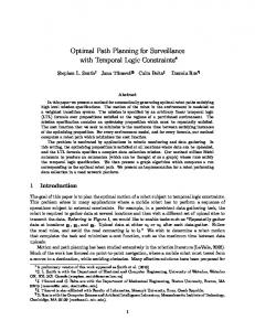
We intend to field the algorithm resulting from this research on the ARL/Penn State flying testbed UAVs.23 The following is a short description of the UAV. The UAV itself is a modified Sig Kadet Senior upgraded with a 0.91 cubic inch four stroke engine. A Piccolo Plus autopilot provides flight control, and an onboard Ampro Readyboard 800 single board computer will handle the path planning tasks. The computer runs a 1.4 GHz Pentium M processor with Windows XP. Currently, a Canon A510 digital camera is used to capture images. In addition to this high resolution camera, a low Figure 1. The fleet of ARL/PSU UAVs. resolution webcam will be installed in order to increase the rate at which images are captured. Both cameras are mounted in a downward orientation and neither is gimbaled. Figure 1 shows a picture of the UAV. Currently, two UAV’s have Piccolo autopilots, but only one is equipped with an onboard computer. The remaining two aircraft are used for training and camera testing. A fifth UAV is under 2 American Institute of Aeronautics and Astronautics

construction; it will carry both the Piccolo autopilot and a single board computer. The goal is to fly two UAVs both running the path planning algorithm to surveil a stationary and moving target. The problem is to generate a path that allows the UAV to track or maintain a camera or some other sensor on a target for as much of the time as possible. This path must be flyable by the UAV, therefore the algorithm must account for the stall speed and maximum turn rate of the aircraft. Additionally, the camera or sensor field of view must be known to determine when the target is in view of the sensor. Of course, given only one UAV and a single target, generating the best flight path for maximum sensor coverage of the target is trivial. Therefore, the main application of this research is in situations involving multiple UAVs and targets, where the paths for maximum sensor coverage are not so obvious. In this situation, we assume that simultaneous sensor coverage of a single target is not advantageous. This assumption can be thought of as an additional constraint: the amount of time a target is covered by multiple sensors should be minimized. Targets will be posterboard of different colors. An image-processing algorithm that uses OpenCV24 recognizes the posterboard in an image. The algorithm first captures an image with a webcam and saves it in the OpenCV image format, IplImage. IplImage stores the red, green, and blue (RGB) pixel values. To account for changes in image brightness (for example, a sunny day versus an overcast day), the RGB values are converted to HSB values (Hue, Saturation, and Brightness). By only considering hue and saturation, the effect of image brightness is removed from the algorithm. Since the posterboard is a solid color, the algorithm defines colored areas instead of individual pixels. The center pixel of a diamond formation of similarly colored pixels is deemed to be of that color. The colored pixels are then grouped into regions by the distance between similarly colored pixels. If only one posterboard is to be found, then the poster is defined as the region with the most pixels in it. Otherwise, multiple posterboards can be identified. If the landscape is relatively flat, a single observation will suffice for target localization because a planar homography can be used. However, if there are local elevation changes as shown in Fig. 2, or for increased accuracy, two or more observations from different locations are required. The planar homography could not be used because the image does not correspond to a plane. To determine the elevation of the target, the equation of the line from the airplane to the target is calculated from a picture by assuming the target elevation is zero and accounting for the attitude of the UAV. Multiple images are captured yielding multiple lines to the target from different Figure 2. World, Aircraft Body, and Image Plane positions. By finding the point closest to all of the coordinate systems collected lines in a least squares sense, the world coordinates of the target can be calculated. Note that our algorithm requires the location of the target to plan an optimal path for observation. This will require a model of target motion that is supplied updates by the above method.

III.

Optimal Path Planning Using DCNLP

A. DCNLP Overview The direct collocation with nonlinear programming is a method for solving optimal control problems with any type of non-linear constraints and objective function. Consider a non-linear dynamic system with a set of non-linear equality and/or inequality constraints

x = f ( x, u ) c ( x, u ) ≤ 0

(1)

where x and u are the state and control input vectors. We seek the control input, u(t), that minimizes some objective function of the form: tf

J = ∫ γ ( x, u )dt t0

3 American Institute of Aeronautics and Astronautics

(2)

In general, any number of the state variables can have their initial values, x(t0), or final values, x(tf), specified, and the final time, tf, can either be specified or be free to vary in the optimization solution. In this paper, we will consider a problem where the initial conditions and final time are specified and the final state vector is free. The DCNLP methods provides an approximate numerical solution to this problem by discretizing the states and controls into a set of equally spaced points in time, called nodes. The state and control trajectories between the nodes are approximated by cubic polynomial functions. In this case, we follow the method presented in ref. 3, using 3rd order Hermite polynomials for the state trajectories and linear interpolation for the controls between nodes. In the case of the states, the Hermite polynomials are defined such that their first derivatives satisfy the state equations at each node: x i = f ( xi , u i ) (3) where the subscript i indicates the value at the ith node. The collocation point is selected as the center of the segment between each node. The objective of the DCNLP method is to search for the optimal solution while ensuring the problem constraints are satisfied and that the equations of motion are satisfied at the collocation point. If the length of a segment is T seconds, then the state vector at the center point of the segment is given by the following equation.

xic = ( xi + xi +1 ) / 2 + (T / 8)[ xi − xi +1 ]

(4)

uic = (ui + ui +1 ) / 2

(5)

The control vector u is given by

To measure the error between the approximating polynomials and the actual equations of motion, a defect vector is defined as

d i = f ( xic , u ic ) − x ic

(6)

xic = −[3 /(2T )]( xi − xi +1 ) − [ xi + xi +1 ] / 4

(7)

where

If the defect vector approaches zero, the polynomials are assumed to be an accurate approximation of the state trajectory as it would be solved from the equations of motion. Of course this will depend on the selection of the time interval T. The specific timescales associated with the equations of motion limit the size of this time interval. Now the problem has been parameterized and the optimal control problem is converted to a non-linear programming (NLP) problem. The parameter vector consists of the state and control vectors at each node

[

X T = x1T

u1T

x 2T

u 2T

" x nT

u nT

]

(8)

and the constraint functions consist of the defect vectors and the problem constraints evaluated at each node:

d1 ( x, u ) = 0 c( x1 , u1 ) ≤ 0 d 2 ( x, u ) = 0 c ( x 2 , u 2 ) ≤ 0 # # d n ( x, u ) = 0 c ( x n , u n ) ≤ 0

(9)

The NLP problem involves searching for the parameter vector (Eq. 8) that minimizes the objective function (Eq. 2) subject to the constraints in Equation 9. The objective function can typically be evaluated using some type of numerical integration along the state and control vectors. There are numerous software packages capable of solving 4 American Institute of Aeronautics and Astronautics

this type of problem using sequential quadratic programming (SQP) methods.21,22 For the simulation results presented in this paper we use the fmincon function from the optimization toolbox in MATLAB®. In future applications on the aircraft, real-time execution speed will be critical, and codes that take advantage of sparse solvers will be desirable.22 B. Equations of Motion In the initial application of this method, we use relatively simple aircraft equations of motion. The aircraft altitude is assumed to be constant and we model only the position kinematics of the aircraft. The control inputs are the commanded forward acceleration and the roll angle. The target is assumed to be moving at constant speed in a straight line on flat terrain, where both its position and velocity are known The problem of estimating the target location and speed and coupling this with the path planning will be the subject of future work, but the initial approach was discussed in Section II. The equations of motion for a single aircraft and a single target are as follows:

x1 = x3 cos( x4 ) x 2 = x3 sin( x4 ) x3 = u1 x 4 = g tan(u 2 ) / x3 x5 = Vtg x

(10)

x 6 = Vtg y In Eq. 5, x1 and x2 are the North and East coordinates of the aircraft, x3 is the aircraft speed, x4 is aircraft heading, x5 and x6 are the North and East coordinates of the target. The control variables, u1 and u2, represent the commanded acceleration and bank angle of the aircraft, which would be regulated by an autopilot system. The equations are readily extended to include multiple aircraft or multiple targets by augmenting the state and control vectors and replicating the equations of motion in Equation 10. Thus for two aircraft and two targets, the complete state vector will have 10 states: four per aircraft and two per target. The aircraft is subject to constraints on speed, bank angle, and acceleration:

Vmin ≤ x3 ≤ Vmax amin ≤ u1 ≤ amax

(11)

φmin ≤ u 2 ≤ φmax These airspeed and acceleration constraints are based on performance limitations and the stall speed of the aircraft. The bank angle limits are based on limitations of the autopilot system. The inclusion of additional constraints is relatively straightforward. For example constraints on aircraft position to provide obstacle / collision / threat avoidance can be readily applied, but are not included in this study. C. Objective Function The objective function is chosen to maximize sensor coverage of the target while minimizing the control effort. The objective function for a single aircraft observing a single target is of the following form:

∫ [W u

tf

J=

2 1 1

(

)

]

+ W1u 22 + W3 ( x1 − x5 ) + ( x2 − x6 ) + W4 J tiv dt 2

2

(12)

t0

The first two terms penalize control effort and the third term weights the square of the distance to the target. The fourth term, Jtiv, is a “Target-in-view” cost function, which has its minimum value when the target is at the center of the image plane of the aircraft camera and reaches its maximum value when the target is out of the camera frame. This function is described in more detail below. Note that the third term (distance to target) is required so that in the case that the target is too far away to be viewed by the aircraft, it will attempt to get closer to the target. In the DCLNP solution the cost function is calculated by performing a numerical integration of equation 12 along the state and control trajectory. The objective function is readily expanded to include cost associated with multiple aircraft by 5 American Institute of Aeronautics and Astronautics

2048 px

North

including additional control effort and distance to target terms. The target-in-view cost can be also expanded to include multiple aircraft as discussed below. The initial time, t0, and state, x(t0), are the current time and state of the aircraft. The optimization is then performed using a receding horizon approach. Receding Horizon Optimization (RHO) methods have been well documented for a variety of control and path planning application. At given intervals, the optimization is performed (using DCNLP) with the current state as the initial condition and the final time selected as some “horizon time”. Only the first part of the control time history from the solution is xa Ψ used, after which the optimization is repeated, and the optimal c path is continuously updated. xim The target-in-view cost is calculated by transforming the target’s world coordinates into image plane coordinates (pixel location, Px and Py) using a homography (see Figure 3). This Ima g X transformation takes into account the attitude of the UAV, its Ce n tee r position relative to the target, the focal length of the camera, the sensor size of the camera, and the orientation of the camera as it is mounted in the airframe. In this formulation we account only for the roll attitude and heading of the aircraft. Pitch attitude is 1536 assumed to be zero, but the effect of pitch could readily be added px Imag ya e Pla c if more detailed equations of motion are used. In this case we also ne yim assume a downward pointing camera, but different camera T orientations could just as easily be analyzed. The target-in-view East Y cost is zero if the target is in the center of the image, varies parabolically to the edge of the image where its maximum value Figure 3. World, Aircraft Body, and is one. Outside of the image bounds, the cost function remains Image Plane coordinate systems equal to one. The target-in-view cost for a single aircraft and a single target is given by the following equation:

J tiv = min(max((2 Px / I x max ) 2 , (2 Py / I y max ) 2 ),1.0)

(13)

where Ixmax and Iymax represent the number of pixels across the image plane. For multiple aircraft performing surveillance on a single target, Jtiv, represents the minimum value of Jtiv for all aircraft. Thus, the cost is based on the aircraft that has the best view of the target and it is assumed that there is no particular benefit to having multiple aircraft observe the target at the same time.

IV.

Results

The results in Sections A-E were generated using MATLAB® based simulations. We also flew two flight tests as described in Section F. The aircraft constraints were chosen based on known performance limitations of the ARL / PSU UAV described in section II and are summarized in Table 1: Constraint Value Stall Speed Vmin = 25 mph (36.7 ft/sec) Maximum Speed Vmax = 60 mph (88.0 ft/sec) Maximum Acceleration amax = 10 ft/sec/sec and Deceleration amin = -10 ft/sec/sec Maximum Bank Angle φmax = 30° φmin = -30° Table 1 – Aircraft Constraints The receding horizon optimization solution used a horizon time of 20 seconds and was updated every 2 seconds. Ten segments (11 nodes) where used in the DCNLP solution. Four different cases are presented. Case 1 is a trivial case where the target is moving faster than the aircraft’s stall speed but less than its maximum speed. Case 2 is a UAV surveilling a stationary target. In case 3, the target is moving slower than the stall speed of the aircraft. Finally, in case 4, there are two UAVs surveilling a stationary target. For the following plots, the target path is shown with solid line marked periodically with a ‘x’ symbol. The UAV path is shown as a dashed line, and the dotted outline is the field of view of the camera corresponding to the same instant in time as the ‘x’ symbol for the target. The initial solution of the optimal path is shown as a set of ‘+’ symbols. The solution is then updated every two seconds during the course of the maneuver. 6 American Institute of Aeronautics and Astronautics

A. Case 1 – Single UAV & Fast Target Figure 4 shows a relatively trivial case in which a target moving faster than stall speed of the aircraft. The trajectory planner plots an intercept course with the target and then matches the target’s speed. The maneuver is 50 seconds long with marks placed every 10 seconds. The optimal trajectory uses maximum speed from the UAV to overtake the target. Note that the optimal path generated by the first run of the path planner varies from the actual path flown by the UAV. This discrepancy is due to the use of receding horizon control. A complete path is generated that covers the horizon time. The UAV only actually flies the initial part of the path. After 2 seconds, a new optimal path is generated using the current aircraft state as the initial conditions. 1500

500

0

Accel. Cmd (ft/s2) Speed (ft/s)

-1000

-500

0

500

1000 1500 East (ft)

2000

2500

3000

3500

100

Roll Cmd (rad)

North (ft)

1000

50 0

0

10

20

30

40

50

0

10

20

30

40

50

0

10

20

30

40

50

10 0 -10 1 0 -1

Time (s)

Figure 4. Case 1 – Single UAV and a fast moving target

7 American Institute of Aeronautics and Astronautics

B. Case 2 – Single UAV & Stationary Target Figure 5 shows the optimal trajectory to surveil a stationary target. The resulting trajectory is a cloverleaf-shaped pattern. Initially, the UAV accelerates to maximum speed to close the distance to the target, and then drops to minimum speed to surveil the target. The cloverleaf pattern develops because of the bottom pointing camera. Because a down-facing non-gimbaled camera is used, the camera points away from the target when the UAV turns toward the target. To produce maximum observation time, the UAV must fly toward the target, level it wings when passing over it, and then double back for another flyover. The camera field of view outline is omitted in this plot for clarity, but the target is not always in the field of view, only during flyovers.

1200

1000

Target

600

400

200

-200

0

200

400 East (ft)

600

800

1000

100

Accel. Cmd (ft/s2)

Speed (ft/s)

0 -400

Roll Cmd (rad)

North (ft)

800

50 0

0

10

20

30

40

50

60

70

80

0

10

20

30

40

50

60

70

80

0

10

20

30

40 Time (s)

50

60

70

80

10 0 -10 1 0 -1

Figure 5. Case 2 – Single UAV and a stationary target

8 American Institute of Aeronautics and Astronautics

C. Case 3 – Single UAV & Slow Target In this case, the target is moving southwest at a speed 32.5 ft/sec, which is slightly slower than the stall speed of the UAV. To maintain image coverage of the target, UAV must follow the target for a time and then turn away and back again to fall behind the target. The behavior would be ideal for convoy following. Figure 6 shows the path and control time histories.

1000 800 600 400

0 -200 -400 -600 -800 -1000 -1000

-500 East (ft)

0

500

100

Accel. Cmd (ft/s2)

Speed (ft/s)

-1500

Roll Cmd (rad)

North (ft)

200

50 0

0

10

20

30

40

50

60

70

80

0

10

20

30

40

50

60

70

80

0

10

20

30

40 Time (s)

50

60

70

80

10 0 -10 1 0 -1

Figure 6. Case 3 – Single UAV and a slow moving target

9 American Institute of Aeronautics and Astronautics

1000

D. Case 4 – UAV Pair & Stationary Target For the fourth case, we consider a pair of identical UAVs equipped with identical cameras. Note that identical equipment is not a requirement to use DCNLP for the optimization. To avoid collisions, one UAV was flown at 300ft and the other at 400ft altitude, although anti-collision constraints could also be included in the problem. The maneuver is 100 seconds in length. Because the target is stationary, the cloverleaf pattern of Case 2 results for each UAV. However, because the optimization considers both aircraft together, the resulting trajectory staggers the passes over the target so that for a majority of the time, only one UAV has the target in view. This behavior is a consequence of the way the target-in-view objective function is set up for multiple aircraft. No specific priority is given to one UAV over another, and there is no benefit to having both aircraft view the target at the same time. Figure 7 shows the path and controls. Figure 8 shows the distance of each UAV to the target. The bolded sections of the lines in Fig. 8 indicate when the target was in view of a particular UAV. Note that the target is alternately covered between aircraft as they pass over. With two UAVs, the target receives sensor coverage almost 100% of the time the UAVs are on location. For the following figures, the camera field of view outline is omitted for clarity. The turn and acceleration commands are similar to case 2 so they are not shown here.

2000

1800

1600

1200 1100

1400

Distance to target (ft)

1000

North (ft)

1200

1000

800

900 800 700 600 500

600

400 300

400

0

20

40

60

80

100

Time (s)

Figure 8. Case 3 – UAV pair and a stationary target where bold lines indicate the target is imaged by the UAV. The offset in distance is due to a difference in altitude.

200

0 0

200

400 East (ft)

600

800

Figure 7. Case 4 – UAV pair and a stationary target

10 American Institute of Aeronautics and Astronautics

E. Case 5 – Single UAV and stationary target with 15 knot west wind Initially, we had not considered the effect of wind on the optimization. However, our firsts few flight tests, discussed in the following section, showed that wind effects were no small issue. The following simulation results show single UAV surveilling a single stationary target with a constant wind of 15 knots from the west. Incorporating wind into the optimization is feasible because the Piccolo autopilot is able to measure wind by comparing GPS ground speed to indicated air speed. The simulation results show that wind may not be an undesirable effect as it allows the UAV to make very tight ground track turns when turning into the wind. The required modifications to the equations of motion only involve subtracting north and east wind components from the x and y position derivative. Only the modified state equations are shown in Eq. 14.

x1 = x3 cos( x4 ) − Vwind _ x

(14)

x 2 = x3 sin( x4 ) − Vwind _ y

As can bee seen in the plot below, the general strategy produced by the optimization is to fly mostly perpendicular to the wind over the target while letting the wind carry it back over the target. When the UAV is too far away from the target, it favors upwind turns to minimize ground track turn radius and downwind drift. Note that the optimization generally avoids downwind turns. When the simulation was initially run with a horizon time of 20 seconds, the path would often diverge causing the UAV to fly long distances away from the target. No amount of weight adjustment would help. We then tried a horizon time of 30 seconds while continuing with 11 collocation points. After an initial divergence, the path settled down to essentially a figure-8 over the target. The figure-8 was oriented perpendicular to the wind. Increased horizon time alleviated the divergence problem because it allowed the optimization plan farther into the future which produced a more cyclical path.

1300

1300

1200 1200

1100

1100

900

North (ft)

North (ft)

1000

800

15 kts wind 1000

700 600 500

900

15 kts wind 800

400 300 300 400 500 600 700 East (ft)

400

500 600 East (ft)

700

Figure 9. Case 5 – Single UAV and a stationary target with a 15 knot west wind, full path on left and a close view of the resulting figure-8 pattern on the right.

11 American Institute of Aeronautics and Astronautics

F. Flight Test Results We attempted two flight tests of the single UAV and stationary target case. Because the conversion of the algorithm from MATLAB® to C++ is not complete at the time of writing, we generated an optimal path offline in MATLAB®. The path was then converted to a series of waypoints for a simple waypoint following control. Both test attempts failed due to a constant 15 knot west wind at the airfield. Failure was caused by not considering wind in the optimization. The path is designed so that the UAV must fly near its turn rate limit assuming no wind. However, the UAV must exceed the constraints with which the path was calculated to remain on the path in the presence of wind. We did build some tolerance in the path, setting the maximum bank angle at 30° (thus limiting turn rate) in the optimization while the actual bank angle limit of the UAV is 40°. Even with this leeway, the UAV was unable to properly follow the path.

V.

Future Work

The main objective of this research is to develop a path planning algorithm that can be used in real time onboard an airborne UAV. While we have flown two flight tests with an offline solution, their results show the need of an online solution. Future work toward this end includes developing or using an existing nonlinear solver in order to achieve faster solution time than MATLAB® currently provides. The algorithm will also be expanded to generate search patterns and research into distributing the algorithm across multiple vehicles will be conducted.

VI.

Conclusion

The use of direct collocation to generate a trajectory that provides maximum surveillance time of a target for one or more UAVs has been successfully demonstrated in simulation. A trivial case wherein the target moves at a speed achievable by the UAV was successfully shown along with slow and stationary target cases. Using two UAVs, the algorithm was able to calculate trajectories that provided near full time coverage of a stationary target once the aircraft arrived on location. DCNLP allows for the use of a relatively complex objective function and set of constraints that incorporates distance to the target, control effort, and whether or not the target is in view of the onboard camera. No specific initial guess were required to reach a solution. However, the method is too slow for real time operation as it is currently implemented in MATLAB®. Existing nonlinear solver package written in C++ or FORTRAN will be applied to may provide a reduction in solution time and real-time implementation. We performed two flight tests with an offline solution for a single UAV and stationary target, but the presence of a steady wind invalidated these offline generated paths.

VII.

Acknowledgements

The authors would like to acknowledge Gregory Sinsley for his help during the flight test portion of the work.

References 1

Dickmanns, E. D. and Well, H., “Approximate solution of optimal control problems using third-order hermite polynomial functions,” Proceedings of the 6th Technical Conference on Optimization Techniques, Springer-Verlag, New York, 1975. 2 Hargraves, C. R. and Paris, S. W., “Direct trajectory optimization using nonlinear programming and collocation,” AIAA J. Guidance, Control, and Dynamics, Vol. 10, No. 4, 1987, pp. 338-342. 3 Enright, P. J. and Conway, B. A., “Optimal Finite-Thrust Spacecraft Trajectories Using Collocation and Nonlinear Programming,” AIAA J. Guidance, Control, and Dynamics, Vol. 14, No. 5, 1991, pp. 981-985. 4 Roh, W. and Kim, Y., “Trajectory optimization for a multi-stage launch vehicle using time finite element and direct collocation methods,” Engineering Optimization, Vol. 34, No. 1, 2002, pp. 15-32. 5 Herman, A. L. and Conway, B. A., “Direct optimization using collocation based on high-order Gauss-Lobatto quadrature rules,” AIAA J. Guidance, Control, and Dynamics, Vol. 19, No. 3, 1996, pp. 592-599. 6 Coverstone-Carroll, V. and Prussing, J. E., “Optimal cooperative power-limited rendezvous with propellant constraints,” Journal of the Astronautical Sciences, Vol. 43, No. 3, 1995, pp. 289-305. 7 Tang, S. and Conway, B. A., “Optimization of low-thrust interplanetary trajectories using collocation and nonlinear programming,” AIAA J. Guidance, Control, and Dynamics, Vol. 18, No. 3, 1995, pp. 599-604. 8 Enright, P. J. and Conway, B. A., “Discrete approximations to optimal trajectories using direct transcription and nonlinear programming,” AIAA J. Guidance, Control, and Dynamics, Vol. 15, No. 4, 1992, pp. 994-1002. 9 Herman, A. L. and Conway, B. A., “Optimal spacecraft attitude control using collocation and nonlinear programming,” AIAA J. Guidance, Control, and Dynamics, Vol. 15, No. 5, 1992, pp. 1287-1289. 10 Horie, K. and Conway, B. A., “Optimal aeroassisted orbital interception,” AIAA J. Guidance, Control, and Dynamics, Vol. 22, No. 5, 1999, pp. 625-631.

12 American Institute of Aeronautics and Astronautics

11 Yamamoto, T. and Kawaguchi, J., “Optimal control and guidance for vehicles gaining altitude under the aerodynamical conditions,” Advances in the Astronautical Sciences, Vol. 117, 2004, pp. 413-426. 12 Horie, K. and Conway, B. A., “Optimization for fighter aircraft vertical-plane maneuvering using poststall flight,”AIAA Journal of Aircraft, Vol. 37, No. 6, 2000, pp. 1017-1021. 13 Komduur, H. J. and Visser, H. G., “Optimization of vertical plane cobralike pitch reversal maneuvers,” AIAA J. Guidance, Control, and Dynamics, Vol. 25, No. 4, 2002, pp. 693-702. 14 Visser, H. G., “Optimization of high angle-of-attack approach to landing trajectories,” Proceedings of the Institution of Mechanical Engineers, Part G: Journal of Aerospace Engineering, Vol. 219, No. 6, 2005, pp. 497-505. 15 Raghunathan, A. U., Gopal, V., Subramanian, D., Biegler, L. T., Samad, T., “Dynamic optimization strategies for threedimensional conflict resolution of multiple aircraft”, AIAA J. Guidance, Control, and Dynamics, Vol. 27, No. 4, 2004, pp. 586594. 16 Goto, N., Kawable, H., “Direct optimization methods applied to a nonlinear optimal control problem,” Mathematics and Computers in Simulation, Vol. 51, No. 6, 2000, pp. 557-577. 17 Zhao, Y. J., “Optimal patterns of glider dynamic soaring,” Optimal Control Applications and Methods, Vol. 25, No. 2, 2004, pp. 67-89. 18 Zhao, Y. J. and Qi, Y. C., “Minimum fuel power dynamic soaring of unmanned aerial vehicles utilizing wind gradients,” Optimal Control Applications and Methods, Vol. 25, 2004, pp. 211-233. 19 Misovec, K., Inanc, T., Wohletz, J., Murray, R. M., “Low-observable nonlinear trajectory generation for unmanned air vehicles,” Proceedings of the 42nd IEEE Conference on Decision and Control, Vol. 3, 2003, pp 3103-3110. 20 Milam, M. B., Mushambi, K., and Murray, R. M., “A new computational approach to real-time trajectory generation for constrained mechanical systems,” Proceedings of the 39th IEEE Conference on Decision and Control, Vol. 1, 2000, pp. 845-851. 21 Gill, P.E., Murray, W., Saunders, M.A., “A projected lagrangian algorithm and its implementation for sparse nonlinear constraints,” Systems Optimization Laboratory, Stanford University, Stanford, CA, TR-SOL-87-12, Oct. 1987. 22 Betts, J.T., and Huffman, W.P., “The application of sparse nonlinear programming to trajectory optimization,” Boeing Computer Services, Seattle, WA, Jan. 1990. 23 Miller, J. A., Minear, P. D., Niessner, A. F., DeLullo, A. M., Geiger, B. G., Long, L. N., and Horn, J. F., “Intelligent Unmanned Air Vehicle Flight Systems,” Infotech@AIAA, 2005. 24 OpenCV, Software Package, Ver. Beta 5, http://www.intel.com/technology/computing/opencv/index.htm, July 2005. 25 Borrelli, F., Subramanian, D., Raghunathan, A. U., and Biegler, L. T., “Techniques for centralized trajectory planning of multiple unmanned aerial vehicles,” Honeywell Laboratories, Honeywell International, Minneapolis, MN, 55418.

13 American Institute of Aeronautics and Astronautics