Hindawi Publishing Corporation Mathematical Problems in Engineering Volume 2016, Article ID 7679165, 9 pages http://dx.doi.org/10.1155/2016/7679165
Research Article Optimal Preview Control for a Class of Linear Continuous Stochastic Control Systems in the Infinite Horizon Jiang Wu,1 Fucheng Liao,1 and Jiamei Deng2 1
School of Mathematics and Physics, University of Science and Technology Beijing, Beijing 100083, China Leeds Sustainability Institute, Leeds Beckett University, Leeds LS2 9EN, UK
2
Correspondence should be addressed to Fucheng Liao;
[email protected] Received 1 July 2016; Accepted 26 September 2016 Academic Editor: Andrzej Swierniak Copyright © 2016 Jiang Wu et al. This is an open access article distributed under the Creative Commons Attribution License, which permits unrestricted use, distribution, and reproduction in any medium, provided the original work is properly cited. This paper discusses the optimal preview control problem for a class of linear continuous stochastic control systems in the infinite horizon, based on the augmented error system method. Firstly, an assistant system is designed and the state equation is translated to the assistant system. Then, an integrator is introduced to construct a stochastic augmented error system. As a result, the tracking problem is converted to a regulation problem. Secondly, the optimal regulator is solved based on dynamic programming principle for the stochastic system, and the optimal preview controller of the original system is obtained. Compared with the finite horizon, we simplify the performance index. We also study the stability of the stochastic augmented error system and design the observer for the original stochastic system. Finally, the simulation example shows the effectiveness of the conclusion in this paper.
1. Introduction Future reference signals or disturbance signals are known in certain circumstances. All the known future information can be utilized by preview control theory to improve the performance of the dynamic system. The original idea of preview control theory is that in order to minimize the error between the reference signals and the controlled terms, not only the past and present information but also the future information should be concentrated on [1–5]. An augmented error system is constructed while designing the optimal preview controller for the discrete system. And also a group of identical equations of future reference signals is added to the augmented error system [6–9]. Since the continuous system is of infinite dimensions, the method in dealing with the discrete condition is no longer useful. In [10], the augmented error system was constructed by differentiating the state equation on both sides, combining with the error equation. According to the maximum principle, the optimal preview controller was obtained by solving a differential equation on reference signals backward in time. This method was extended to systems with previewable disturbance signals in [11] and to singular continuous systems in [12]. The
application of preview control method to continuous systems with time delay is studied in [13]. According to automatic control system theory, the controlled systems can be regarded as falling into two categories: deterministic systems and stochastic systems. Stochastic systems are a collection of dynamic systems that contain internal stochastic parameters, external stochastic disturbances, or observation noises [14]. A typical stochastic system is the stochastic differential equation. It is a class of differential equations driven by one or more stochastic processes. Therefore, the solution of a stochastic differential equation is also a stochastic process. Up to the present, a phenomenon such as stock market volatility or thermal motion in a physical system is usually described by a stochastic differential equation. Typically, a white noise stochastic variable represented by the differential form of Brownian motion or Weiner process is contained in a stochastic differential equation. In this paper, preview control theory is applied to a class of linear continuous stochastic control systems in the infinite horizon. In the finite horizon [15], an assistant system is designed, and the state equation is translated to the assistant system. Then an integrator is introduced to construct a stochastic augmented error system. As a result, the tracking
2
Mathematical Problems in Engineering
problem is converted to a regulation problem. The optimal regulator is obtained based on the dynamic programming principle for stochastic systems, which means the optimal preview controller of the original stochastic system is gained. For such a system, when the integrator approaches zero at infinity, the error also approaches zero. Therefore, this property can be utilized to simplify the performance index in the infinite horizon. Due to the fact that the relative terms of reference signals are included in the stochastic augmented error system, the conclusion in the infinite horizon cannot be directly employed when solving the optimal regulation problem in this paper. Firstly, the corresponding optimal regulation problem is solved in the finite horizon with the new performance index and then the time was set to approach infinity. The stability of the stochastic augmented error system is studied and the sufficient and necessary criteria which guarantee that there exists a unique semipositive definite solution to the corresponding Riccati equation have been met. Also an observer for the original stochastic system is designed. The introduction of the integrator can eliminate the static error and the simulation example shows the effectiveness of the conclusion in this paper [16]. Notation. The notations are standard. (Ω, 𝐹, 𝑃) is a complete probability space. Adaptive procedure 𝐹𝑡 is 𝜎 algebra generated by {𝐵𝑠 : 𝑠 ≤ 𝑡}, and 𝐵𝑠 denotes Brownian motion of 𝑚 dimensions. 𝐴 ∈ 𝑅𝑚×𝑛 denotes 𝑚 × 𝑛 matrix. 𝑃 > 0 (𝑃 ≥ 0) denotes a positive definite (semidefinite) matrix. 𝐼 denotes the unit matrix. The symbol ∗ denotes the symmetric terms in a symmetric matrix. 𝐸𝑡0 ,𝑥0 denotes the expectation of process (𝑡, 𝑥) with initial time 𝑡0 and state 𝑥0 . tr(⋅) denotes the trace of a matrix.
2. Problem Statement
Remark 4. Since there are few effects on the system when the reference signals exceed the previewable range, it is always assumed that the signals are usually constant [11]. The tracking error signal 𝑒(𝑡) is defined as the difference between the output vector 𝑦(𝑡) and the reference signal 𝑟(𝑡); that is, 𝑒 (𝑡) = 𝑦 (𝑡) − 𝑟 (𝑡) .
(2)
In this paper, an optimal controller will be designed to make the output 𝑦(𝑡) in (1) tracking the reference signal 𝑟(𝑡) as accurately as possible without static error. Then, an assistant system is defined. The following assumption is needed. Assumption 5. Suppose 𝑀 𝑁 ] = 𝑚 + 𝑝, (full row rank) . 𝐶 0
rank [
(3)
With Assumption 5, the following lemma holds. Lemma 6 (see [15]). There exist matrices pairs (Γ, 𝛾) which solve the following: 𝑀Γ + 𝑁𝛾 = 0, 𝐶Γ = 𝐼,
(4)
if and only if Assumption 5 holds, where Γ ∈ 𝑅𝑚×𝑝 and 𝛾 ∈ 𝑅𝑛×𝑝 . Definition 7 (see [17]). If matrix 𝐴 ∈ 𝑅𝑚×𝑛 and the rank of 𝐴 is equal to 𝑛, then 𝐴 has a left inverse: 𝐵 ∈ 𝑅𝑛×𝑚 such that 𝐵𝐴 = 𝐼.
Consider the following stochastic control system: 𝑑𝑥 (𝑡) = [𝑀𝑥 (𝑡) + 𝑁𝑢 (𝑡)] 𝑑𝑡 + 𝜔 (𝑡) 𝑑𝐵𝑡 , 𝑦 (𝑡) = 𝐶𝑥 (𝑡) ,
Moreover, 𝑟(𝜌) (𝑡 ≤ 𝜌 ≤ 𝑡 + 𝑙𝑟 ) is available at any moment ̇ = 0. 𝑙𝑟 is 𝑡 and when 𝜌 > 𝑡 + 𝑙𝑟 , 𝑟(𝜌) = 𝑟(𝑡 + 𝑙𝑟 ); that is, 𝑟(𝜌) the preview length of the reference signal.
(1) 𝑥 (𝑡0 ) = 𝑥0 , 𝑡 ∈ [𝑡0 , ∞) ,
where 𝑥(𝑡) is the state vector of 𝑚 dimensions, 𝑦(𝑡) is the output vector of 𝑝 dimensions, 𝑢(𝑡) is the 𝐹𝑡 adaptive input of 𝑛 dimensions, and 𝐵𝑡 is the Brownian motion of 𝐹𝑡 adaptive of 𝑚 dimensions. 𝑀 ∈ 𝑅𝑚×𝑚 , 𝑁 ∈ 𝑅𝑚×𝑛 , and 𝐶 ∈ 𝑅𝑝×𝑚 are constant matrices. 𝜔(𝑡) ∈ 𝑅𝑚×𝑚 . First of all, the following assumptions are introduced. Assumption 1. Suppose the matrices pair (𝑀, 𝑁) is stabilizable. Assumption 2. Suppose the matrices pair (𝐶, 𝑀) is detectable and the matrix 𝐶 is of full row rank. By denoting the reference signals of 𝑝 dimensions with 𝑟(𝑡), another assumption about 𝑟(𝑡) is needed. Assumption 3. Suppose the reference signal 𝑟(𝑡) is a piecewise continuously differentiable function defined on (𝑡 ≥ 𝑡0 ).
Remark 8. If 𝑝 = 𝑛, there exists unique solution of matrices pair (Γ, 𝛾), while if 𝑝 < 𝑛, according to Definition 7, any 𝑁 left inverse of matrix [ 𝑀 𝐶 0 ] can be applied to calculate the solution of (4) and the solutions are infinite. In this paper only the square full-rank case is used. Let the state vector and input vector be denoted by 𝑥∗ (𝑡) and 𝑢∗ (𝑡), respectively. Let 𝑥∗ (𝑡) = Γ𝑟(𝑡 + 𝑙𝑟 ) and 𝑢∗ (𝑡) = 𝛾𝑟(𝑡 + 𝑙𝑟 ). According to Lemma 6, at the moment 𝑠, for any time 𝑡 (𝑠 ≤ 𝑡 ≤ 𝑡𝜏 ), 𝑥∗ (𝑡) meets 𝑑𝑥∗ (𝑡) = Γ𝑟̇ (𝑡 + 𝑙𝑟 ) 𝑑𝑡, 𝐶𝑥∗ (𝑡) = 𝐶Γ𝑟 (𝑡 + 𝑙𝑟 ) .
(5)
Since [𝑀Γ + 𝑁𝛾]𝑟(𝑡 + 𝑙𝑟 ) = 0 and 𝐶Γ𝑟(𝑡 + 𝑙𝑟 ) = 𝑟(𝑡 + 𝑙𝑟 ) according to (4), substituting these two equations into (5) yields 𝑑𝑥∗ (𝑡) = {[𝑀Γ + 𝑁𝛾] 𝑟 (𝑡 + 𝑙𝑟 ) + Γ𝑟̇ (𝑡 + 𝑙𝑟 )} 𝑑𝑡, 𝑟 (𝑡 + 𝑙𝑟 ) = 𝐶𝑥∗ (𝑡) ;
(6)
Mathematical Problems in Engineering
3
3. Construction of the Stochastic Augmented Error System
that is, ∗
∗
∗
𝑑𝑥 (𝑡) = {[𝑀𝑥 (𝑡) + 𝑁𝑢 (𝑡)] + Γ𝑟̇ (𝑡 + 𝑙𝑟 )} 𝑑𝑡, 𝑟 (𝑡 + 𝑙𝑟 ) = 𝐶𝑥∗ (𝑡) .
(7)
Combining (9) and (11), the following holds: ̃ (𝑡) + 𝑁̃ ̃ 𝑢 (𝑡) + 𝐷̃ ̃ 𝑟 (𝑡) + Γ̃𝑟̇ (𝑡 + 𝑙𝑟 )] 𝑑𝑡 𝑑𝑧 (𝑡) = [𝑀𝑧
Define ∗
̃ (𝑡) = 𝑥 (𝑡) − 𝑥 (𝑡) , 𝑥 ̃ (𝑡) = 𝑢 (𝑡) − 𝑢∗ (𝑡) , 𝑢 ∗
̃ (𝑡) = 𝑦 (𝑡) − 𝐶𝑥 (𝑡) , 𝑦
+ 𝜔 (𝑡) 𝑑𝐵𝑡 , (8)
where
], 0 𝑀
0 ̃ = [ ], 𝑁 𝑁
(9)
̃=[ 𝐷
̃ (𝑡0 ) = 𝑥0 − 𝑥∗ (𝑡0 ) , 𝑡 ∈ [𝑡0 , ∞) . 𝑥 Now an integrator is introduced. Integrating the tracking error signal 𝑒(𝑡) in the interval of 𝑡0 to 𝑡 yields 𝑡
𝑡0
𝑡0
𝑞 (𝑡) = ∫ 𝑒 (𝑠) 𝑑𝑠 = ∫ [𝑦 (𝑠) − 𝑟 (𝑠)] 𝑑𝑠.
(10)
𝑡
Obviously 𝑞(𝑡0 ) = 0. Let 𝑞∗ (𝑡) = ∫𝑡 [𝐶𝑥∗ (𝑠) − 𝑟(𝑠 + 𝑙𝑟 )]𝑑𝑠, and 0 then 𝑞∗ (𝑡) = 0 holds. Define 𝑞̃(𝑡) = 𝑞(𝑡) − 𝑞∗ (𝑡) and the differential form of 𝑞̃(𝑡) becomes 𝑑̃𝑞 (𝑡) = 𝑒 (𝑡) 𝑑𝑡 = [𝐶̃ 𝑥 (𝑡) − ̃𝑟 (𝑡)] 𝑑𝑡.
(11)
Remark 9. According to Assumption 3, the term ̃𝑟(𝑡) in (11) is also previewable while ̃𝑟(𝜌) (𝑡 ≤ 𝜌 ≤ 𝑡 + 𝑙𝑟 ). In particular, while 𝜌 ≥ 𝑡 + 𝑙𝑟 , ̃𝑟(𝜌) = 0. In order to make the output 𝑦(𝑡) tracking the reference signal 𝑟(𝑡) as accurately as possible, the performance index 𝐽 is designed as
Γ̃ = [
where 𝑄𝑞̃ = 𝑄𝑞̃𝑇 > 0 and 𝑅 = 𝑅𝑇 > 0 are matrices of proper dimensions. Remark 10. Compared with the finite horizon, lim𝑡→∞ 𝑒(𝑡) = 0 can also be obtained in the infinite horizon while lim𝑡→∞ 𝑞(𝑡) = 0. Therefore, the term 𝑒𝑇 (𝑡)𝑄𝑒 𝑒(𝑡) in the performance index of [15] can be replaced by 𝑞̃𝑇 (𝑡)𝑄𝑞̃ 𝑞̃(𝑡) in (12). Furthermore, since there exists unique semipositive definite solution of the corresponding Riccati equation when 𝑄𝑞̃ > 0, no other terms need to be included in the performance index, which simplifies the calculation. To solve the optimal control problem of (9) with the performance index (12), the augmented error system method can be employed.
−𝐼 0
(14)
],
0
]. −Γ
Referring to the output equation of (9) and the reference signal, the output of (13) can be defined as ̃ (𝑡) , 𝑞̃ (𝑡) = 𝐶𝑧
(15)
̃ = [𝐼 0]. Joining (13) and (15) together, the following where 𝐶 hold: ̃ (𝑡) + 𝑁̃ ̃ 𝑢 (𝑡) + 𝐷̃ ̃ 𝑟 (𝑡) + Γ̃𝑟̇ (𝑡 + 𝑙𝑟 )] 𝑑𝑡 𝑑𝑧 (𝑡) = [𝑀𝑧 + 𝜔 (𝑡) 𝑑𝐵𝑡 , ̃ (𝑡) , 𝑞̃ (𝑡) = 𝐶𝑧
(16) 𝑞̃ (𝑡0 ) ] = 𝑧0 . 𝑧 (𝑡0 ) = [ ̃ 0 (𝑡0 ) 𝑥
̃ (⋅)) 𝐽 (𝑡0 , 𝑥0 ; 𝑢 (12) 1 ∞ ̃ 𝑇 (𝑡) 𝑅̃ 𝑢 (𝑡)] 𝑑𝑡} , = 𝐸𝑡0 ,𝑥0 { ∫ [̃𝑞𝑇 (𝑡) 𝑄𝑞̃ 𝑞̃ (𝑡) + 𝑢 2 𝑡0
],
̃=[ 𝑀
𝑑̃ 𝑥 (𝑡) = [𝑀̃ 𝑥 (𝑡) + 𝑁̃ 𝑢 (𝑡) + (−Γ) 𝑟̇ (𝑡 + 𝑙𝑟 )] 𝑑𝑡
𝑡
̃ (𝑡) 𝑥
0 𝐶
Subtracting (7) by (1) from both sides, the following could be obtained:
̃ (𝑡) = 𝐶̃ 𝑦 𝑥 (𝑡) ,
𝑞̃ (𝑡)
𝑧 (𝑡) = [
̃𝑟 (𝑡) = 𝑟 (𝑡) − 𝑟 (𝑡 + 𝑙𝑟 ) .
+ 𝜔 (𝑡) 𝑑𝐵𝑡 ,
(13)
Equation (16) is the needed stochastic augmented error system.
4. Design of the Optimal Controller for the Stochastic System Denoting the performance index (12) with the related variables in (16) yields 1 ̃𝐽 (𝑡0 , 𝑧0 ; 𝑢 ̃ (⋅)) = 𝐸𝑡0 ,𝑧0 { 2 ∞
̃ 𝑧 (𝑡) + 𝑢 ̃𝑇 𝑄𝑞̃ 𝐶) ̃ 𝑇 (𝑡) 𝑅̃ ⋅ ∫ [𝑧 (𝑡) (𝐶 𝑢 (𝑡)] 𝑑𝑡} .
(17)
𝑇
𝑡0
̃ 𝑟(𝑡) + Γ̃𝑟(𝑡 ̇ + 𝑙𝑟 ) in Due to the existence of the term 𝐷̃ (16), the conclusion of the optimal regulation problem in
4
Mathematical Problems in Engineering
dealing with the infinite horizon cannot be directly employed. Therefore, similar to the condition in deterministic systems [11], the optimal regulator of the stochastic augmented error system (16) can be obtained through the following three steps. Firstly, (17) is revised to ̃𝐽 = lim 𝐸𝑡0 ,𝑧0 { 1 𝑡𝜏 →∞ 2 𝑡𝜏
(18)
𝑇
̃ 𝑄𝑞̃ 𝐶𝑧 ̃ (𝑡) + 𝑢 ̃ (𝑡) 𝑅̃ 𝑢 (𝑡)] 𝑑𝑡} . ⋅ ∫ [𝑧 (𝑡) 𝐶 𝑇
𝑇
̃ ×̃ 𝑚 is the unique semipositive definite solution of where 𝑃 ∈ 𝑅𝑚 Riccati differential equation
̃ 𝑇𝑃 + 𝐶 ̃ = 0. ̃ − 𝑃𝑁𝑅 ̃ −1 𝑁 ̃𝑇 𝑄𝑞̃ 𝐶 ̃ 𝑇 𝑃 + 𝑃𝑀 𝑀
̃ 𝑁) ̃ is Proof. In terms of the performance index (17), if (𝑀, ̃ 𝑀) ̃ is detectable, according to the stabilizable and (𝑄𝑞̃1/2 𝐶, known conclusion, there exists a unique semipositive definite solution 𝑃 of Riccati algebra equation
𝑡0
Secondly, the finite-time horizon optimal regulation problem with the performance index ̃̃𝐽 = 𝐸𝑡0 ,𝑧0 { 1 2 𝑡𝜏
𝑇
𝑡0
is solved, where 𝑡𝜏 is the terminal time. Compared with the performance index in [15], the two terms 𝑒𝑇 (𝑡)𝑄𝑒 𝑒(𝑡) and 𝑒𝑇 (𝑡𝜏 )𝑄𝑒(𝑡𝜏 ) 𝑒(𝑡𝜏 ) are removed in (19). Therefore, according to the dynamic programming principle for stochastic systems [16, 18], the following lemma about the finite horizon optimal control problem with the terminal time 𝑡𝜏 can be obtained by letting 𝑄𝑒 = 𝑄𝑒(𝑡𝜏 ) = 0 in Theorem 1 in [15]. Lemma 11 (see [15]). If Assumptions 3 and 5 hold, the optimal controller of (16), with the performance index (19), is 𝑇
̃ {𝑃 (𝑡) 𝑧 (𝑡) + 𝜃 (𝑡)} , ̃ (𝑡) = −𝑅−1 𝑁 𝑢 1 (𝑚+𝑝)×(𝑚+𝑝)
where 𝑃(𝑡) ≥ 0 ∈ 𝑅 equation
(20)
𝑇
lim 𝑃 (𝑡) = 𝑃.
𝑇
As a result, the solving of 𝜃(𝑡) in (22) is also simplified. ̃ 𝑇 𝑃. Equation (22) and its term̃ 𝑁𝑅 ̃ −1 𝑁 Denote 𝑀𝑐 = 𝑀− inal condition can be expressed as ̃ 𝑟 (𝑡) + 𝑃Γ̃𝑟̇ (𝑡 + 𝑙𝑟 )) = 0, 𝜃̇ (𝑡) + 𝑀𝑐𝑇 𝜃 (𝑡) + (𝑃𝐷̃ 𝜃 (𝑡𝜏 ) = 0.
̃ 𝑇 ) 𝜃 (𝑡) ̃ 𝑇 − 𝑃 (𝑡) 𝑁𝑅 ̃ −1 𝑁 𝜃̇ (𝑡) + (𝑀 ̃ 𝑟 (𝑡) + 𝑃 (𝑡) Γ̃𝑟̇ (𝑡 + 𝑙𝑟 )) = 0, + (𝑃 (𝑡) 𝐷̃
𝑡
̃ (𝑡, 𝑡0 ) = exp [− ∫ 𝑀𝑇 𝑑𝑡] = exp [(𝑡0 − 𝑡) 𝑀𝑇 ] , Φ 𝑐 𝑐 𝑡0
̃ (𝑡, 𝑡0 ) , ̃ −1 (𝑡0 , 𝑡) = Φ Φ
𝑡0 ≤ 𝑠 ≤ 𝑡. Therefore, the solution of (27) is ̃ (𝑡, 𝑡0 ) 𝜃 (𝑡0 ) 𝜃 (𝑡) = Φ 𝑡
̃ (𝑡, 𝑠) (𝑃𝐷̃ ̃ 𝑟 (𝑡) + 𝑃Γ̃𝑟̇ (𝑡 + 𝑙𝑟 )) 𝑑𝑠, −∫ Φ
(30)
̃ (𝑡𝜏 , 𝑡) 𝜃 (𝑡) 𝜃 (𝑡𝜏 ) = Φ
𝑇
̃ 𝑃𝑧 (𝑡) ̃ (𝑡) = −𝑅−1 𝑁 𝑢 𝑇
̃ 𝑇 𝑃) ] ̃ − 𝑁𝑅 ̃ −1 𝑁 exp [(𝑡0 − 𝑡) (𝑀
̃ 𝑟 (𝑠) + 𝑃Γ̃𝑟̇ (𝑠 + 𝑙𝑟 )) 𝑑𝑠, ⋅ (𝑃𝐷̃
(29)
and the backward form is
Theorem 12. If Assumptions 1 to 5 hold, the optimal controller ̃ (𝑡) of (16) with the performance index (17) can be expressed 𝑢 as
𝑡
̃ (𝑡, 𝑡0 ) = Φ ̃ (𝑡, 𝑡𝑠 ) Φ ̃ (𝑡𝑠 , 𝑡0 ) , Φ
𝑡0
Thirdly, Theorem 12 is received by letting 𝑡𝜏 → ∞.
𝑡+𝑙𝑟
(28)
with the property
(22)
with the terminal condition 𝜃(𝑡𝜏 ) = 0.
̃ ∫ − 𝑅−1 𝑁
(27)
Based on linear system theory [19], the fundamental solution matrix of the homogeneous system corresponding to (27) is
(21)
With the terminal condition 𝑃(𝑡𝜏 ) = 0 and 𝜃(𝑡) the differential equation is obtained:
(26)
𝑡→∞
𝑇
̃ ̃ 𝑄𝑞̃ 𝐶. +𝐶
(25)
And when 𝑡 → ∞,
satisfies the Riccati differential
̃ 𝑃𝑇 (𝑡) ̃ 𝑃 (𝑡) + 𝑃 (𝑡) 𝑀 ̃ − 𝑃 (𝑡) 𝑁𝑅 ̃ −1 𝑁 −𝑃̇ (𝑡) = 𝑀
𝑇
̃ 𝑇𝑃 + 𝐶 ̃ = 0. ̃ 𝑇 𝑃 + 𝑃𝑀 ̃ − 𝑃𝑁𝑅 ̃ −1 𝑁 ̃𝑇 𝑄𝑞̃ 𝐶 𝑀
(19)
̃ 𝑄𝑞̃ 𝐶𝑧 ̃ (𝑡) + 𝑢 ̃ 𝑇 (𝑡) 𝑅̃ 𝑢 (𝑡)] 𝑑𝑡} ⋅ ∫ [𝑧𝑇 (𝑡) 𝐶
(24)
(23)
𝑡𝜏
̃ (𝑡𝜏 , 𝑠) (𝑃𝐷̃ ̃ 𝑟 (𝑠) + 𝑃Γ̃𝑟̇ (𝑠 + 𝑙𝑟 )) 𝑑𝑠. −∫ Φ
(31)
𝑡
With the terminal condition 𝜃(𝑡𝜏 ) = 0, the following will be obtained: 𝜃 (𝑡) 𝑡𝜏
̃ (𝑡𝜏 , 𝑠) (𝑃𝐷̃ ̃ 𝑟 (𝑠) + 𝑃Γ̃𝑟̇ (𝑠 + 𝑙𝑟 )) 𝑑𝑠. ̃ −1 (𝑡𝜏 , 𝑡) ∫ Φ =Φ 𝑡
(32)
Mathematical Problems in Engineering
5
According to the property of the reference signals in Assumption 3, 𝜃(𝑡) can be expressed as ̃ −1 (𝑡𝜏 , 𝑡) 𝜃 (𝑡) = Φ ⋅∫
𝑡𝜏 ∧(𝑡+𝑙𝑟 )
𝑡
𝑡𝜏 ∧(𝑡+𝑙𝑟 )
𝑡
=∫
Corollary 14. If Assumptions 1 to 5 hold, the optimal preview controller 𝑢(𝑡) of (1) with the performance index (12) can be expressed as
̃ (𝑡𝜏 , 𝑠) (𝑃𝐷̃ ̃ 𝑟 (𝑠) + 𝑃Γ̃𝑟̇ (𝑠 + 𝑙𝑟 )) 𝑑𝑠 Φ
𝑇
(33) 𝑇
̃ ∫ − 𝑅−1 𝑁
̃ (𝑡𝜏 , 𝑠) (𝑃𝐷̃ ̃ 𝑟 (𝑠) + 𝑃Γ̃𝑟̇ (𝑠 + 𝑙𝑟 )) 𝑑𝑠 Φ
𝑡𝜏 ∧(𝑡+𝑙𝑟 )
𝑡
𝑇
𝑇
𝑡𝜏 ∧(𝑡+𝑙𝑟 )
𝑡
̃ (𝑡, 𝑠) Φ
(34)
where 𝑡𝜏 ∧ (𝑡 + 𝑙𝑟 ) = min{𝑡𝜏 , 𝑡 + 𝑙𝑟 }. The conclusion is that when 𝑡𝜏 → ∞, the following theorem can be obtained. Theorem 13. If Assumptions 1 to 5 hold, the optimal controller ̃ (𝑡) of (16) with the performance index (17) can be expressed 𝑢 as ̃ (𝑡) 𝑢 𝑇
𝑇
(35)
𝑡+𝑙𝑟
̃ (𝑡, 𝑠) (𝑃𝐷̃ ̃ 𝑟 (𝑠) + 𝑃Γ̃𝑟̇ (𝑠 + 𝑙𝑟 )) 𝑑𝑠, Φ
𝑡
̃ ×̃ 𝑚 where 𝑃 ∈ 𝑅𝑚 is the unique semipositive definite solution of Riccati differential equation 𝑇
−1 ̃ 𝑇
𝑇
̃ = 0. ̃ − 𝑃𝑁𝑅 ̃ 𝑁 𝑃+𝐶 ̃ 𝑄𝑞̃ 𝐶 ̃ 𝑃 + 𝑃𝑀 𝑀
(36)
−1 ̃ 𝑇
𝑇
𝑡+𝑙𝑟
𝑡
−1 ̃ 𝑇
∗
̃ (𝑡, 𝑠) 𝑃𝐷̃ ̃ 𝑟 (𝑠) 𝑑𝑠 + 𝑢∗ (𝑡) Φ −1 ̃ 𝑇
With 𝜔(𝑡)𝑑𝐵𝑡 being an external disturbance, the stability and detectability of system (16) are studied only when 𝜔(𝑡) = 0. Here, (16) becomes the deterministic system ̃ (𝑡) + 𝑁̃ ̃ 𝑢 (𝑡) + 𝐷̃ ̃ 𝑟 (𝑡) + Γ̃𝑟̇ (𝑡 + 𝑙𝑟 )] 𝑑𝑡. 𝑑𝑧 (𝑡) = [𝑀𝑧
(40)
As a result, the sufficient and necessary criteria which guarantee that there exists a unique semipositive definite solution to the Riccati equation (24) can be gained by the known conclusion, as follows. Lemma 15 (see [11]). Suppose the following conditions are satisfied:
𝑀 𝑁 ] Π=[ 𝐶 0 ] [
(41)
is of full row rank. (3) The matrices pair (𝑀, 𝑁) is stabilizable.
𝑢 (𝑡) = −𝑅 𝑁 𝑃1 𝑞 (𝑡) − 𝑅 𝑁 𝑃2 𝑥 (𝑡) ̃ ∫ − 𝑅−1 𝑁
5. Stability of Closed-Loop System
(2) The matrix (37)
̃ × 𝑝 and 𝑚 ̃ × 𝑚. According to where 𝑃1 and 𝑃2 are matrices of 𝑚 𝑡+𝑙𝑟 𝑞̃(𝑡) ̃ ̃ ̇ + 𝑙𝑟 )𝑑𝑠 = 0, the (8), (35), 𝑧(𝑡) = [ 𝑥̃(𝑡) ], and ∫𝑡 Φ(𝑡, 𝑠)𝑃Γ𝑟(𝑠 following will be obtained: −1 ̃ 𝑇
From (39) it can be seen that there are four parts contained in the preview controller of (1): the first part is the intẽ 𝑇 𝑃1 𝑞(𝑡), stemmed from the gral of tracking error term −𝑅−1 𝑁 inducing of the integrator. The second part is the state feed̃ 𝑇 𝑃2 𝑥(𝑡). The third one −𝑅−1 𝑁 ̃ 𝑇 ∫𝑡+𝑙𝑟 Φ(𝑡, ̃ back −𝑅−1 𝑁 𝑡 ̃ 𝑠)𝑃𝐷̃𝑟(𝑠)𝑑𝑠 is the reference preview compensation. The last ̃ 𝑇 𝑃2 Γ]𝑟(𝑡 + 𝑙𝑟 ) is the previewable complement one [𝛾 + 𝑅−1 𝑁 of the assistant system.
(1) The matrices 𝑄𝑞̃ and 𝑅 are both positive definite.
Then, let the matrix 𝑃 be separated into 𝑃 = [𝑃1 𝑃2 ] ,
(39)
𝑇
̃ 𝑟 (𝑠) + 𝑃Γ̃𝑟̇ (𝑠 + 𝑙𝑟 )) 𝑑𝑠, ⋅ (𝑃𝐷̃
̃ 𝑃𝑧 (𝑡) = −𝑅−1 𝑁
̃ (𝑡, 𝑠) 𝑃𝐷̃ ̃ 𝑟 (𝑠) 𝑑𝑠 Φ
̃ 𝑃2 Γ] 𝑟 (𝑡 + 𝑙𝑟 ) . + [𝛾 + 𝑅−1 𝑁
̃ (𝑡, 𝑠) (𝑃𝐷̃ ̃ 𝑟 (𝑠) + 𝑃Γ̃𝑟̇ (𝑠 + 𝑙𝑟 )) 𝑑𝑠. Φ
̃ 𝑃𝑧 (𝑡) − 𝑅−1 𝑁 ̃ ∫ ̃ (𝑡) = −𝑅−1 𝑁 𝑢 1
𝑡+𝑙𝑟
𝑡
Substituting (33) into (20) yields
̃ ∫ − 𝑅−1 𝑁
𝑇
̃ 𝑃1 𝑞 (𝑡) − 𝑅−1 𝑁 ̃ 𝑃2 𝑥 (𝑡) 𝑢 (𝑡) = −𝑅−1 𝑁
̃ (𝑡, 𝑡𝜏 ) =Φ ⋅∫
Due to the fact that 𝑥∗ (𝑡) = Γ𝑟∗ (𝑡 + 𝑙𝑟 ), 𝑢∗ (𝑡) = 𝛾𝑟∗ (𝑡 + 𝑙𝑟 ), and 𝑞∗ (𝑡) = 0, the following corollary is obtained.
(4) The matrices pair (𝐶, 𝑀) is detectable. (38)
∗
+ 𝑅 𝑁 𝑃2 𝑞 (𝑡) + 𝑅 𝑁 𝑃2 𝑥 (𝑡) , ̃ ×̃ 𝑚 where 𝑃 ≥ 0 ∈ 𝑅𝑚 satisfies Riccati differential equation (24).
Then there exists unique semipositive definite solution in the Riccati equation (24), and there exists the asymptotically stable coefficient matrix 𝑀𝑐 in the closed-loop system (27). Therefore, the following theorem can be received.
6
Mathematical Problems in Engineering
Theorem 16. If 𝑄𝑞̃ and 𝑅 are both positive definite matrices and Assumptions 1 to 5 hold, the full regulation is achieved in the closed-loop system: 𝑑𝑧 (𝑡)
Theorem 17. If the conditions in Theorem 16 hold, the closedloop system can be received: 𝑑𝑥 (𝑡) = [𝑀𝑥 (𝑡) + 𝑁𝑢 (𝑡)] 𝑑𝑡 + 𝜔 (𝑡) 𝑑𝐵𝑡 , 𝑑̂ 𝑥 (𝑡) = [𝑀̂ 𝑥 (𝑡) + 𝑁𝑢 (𝑡) + 𝐿 (𝑦 (𝑡) − 𝐶̂ 𝑥 (𝑡))] 𝑑𝑡
̃ (𝑡) + 𝑁̃ ̃ 𝑢 (𝑡) + 𝐷̃ ̃ 𝑟 (𝑡) + Γ̃𝑟̇ (𝑡 + 𝑙𝑟 )] 𝑑𝑡 = [𝑀𝑧
+ 𝜔 (𝑡) 𝑑𝐵𝑡 , 𝑦 (𝑡) = 𝐶𝑥 (𝑡) ,
+ 𝜔 (𝑡) 𝑑𝐵𝑡 , ̃ (𝑡) 𝑢
𝑡
𝑇
̃ 𝑃1 ∫ (𝐶̂ 𝑥 (𝑠) − 𝑟 (𝑠)) 𝑑𝑠 𝑢 (𝑡) = −𝑅−1 𝑁 𝑡0
−1 ̃ 𝑇
= −𝑅 𝑁 𝑃𝑧 (𝑡) 𝑇
̃ ∫ − 𝑅−1 𝑁
𝑡+𝑙𝑟
𝑡
(42)
(48)
𝑇
̃ 𝑃2 𝑥 ̂ (𝑡) − 𝑅−1 𝑁
̃ (𝑡, 𝑠) (𝑃𝐷̃ ̃ 𝑟 (𝑠) + 𝑃Γ̃𝑟̇ (𝑠 + 𝑙𝑟 )) 𝑑𝑠, Φ
𝑇
̃ ∫ − 𝑅−1 𝑁
̃ (𝑡) 𝑞̃ (𝑡) = 𝐶𝑧
𝑡+𝑙𝑟
𝑡
̃ (𝑡, 𝑠) 𝑃𝐷̃ ̃ 𝑟 (𝑠) 𝑑𝑠 Φ
𝑇
̃ 𝑃2 Γ] 𝑟 (𝑡 + 𝑙𝑟 ) , + [𝛾 + 𝑅−1 𝑁
𝑞̃ (𝑡0 )
] = 𝑧0 ; 𝑧 (𝑡0 ) = [ ̃ 0 (𝑡0 ) 𝑥
where (𝑀 − 𝐿𝐶) is stable and (48) achieve the complete regulation.
namely, lim 𝑞̃ (𝑡) = 0.
𝑡→∞
7. Numerical Simulation (43)
Furthermore, the following will be obtained: lim 𝑒 (𝑡) = 0.
𝑡→∞
Example 1. Consider the stochastic control system 𝑑[
(44)
𝑥1 (𝑡) 𝑥2 (𝑡)
] = [[
0
1
−1 −1
𝑥1 (𝑡)
][
0 ] + [ ] 𝑢 (𝑡)] 𝑑𝑡 1 𝑥2 (𝑡)
+ 0.1 𝑑𝐵𝑡 , 𝑥1 (𝑡)
6. State Observer
𝑦 (𝑡) = [1 0] [
If the state vector 𝑥(𝑡) in (1) cannot be measured directly, the optimal preview controller (39) cannot be realized. In order to solve this problem, the state observer 𝑑̂ 𝑥 (𝑡) = [𝑀̂ 𝑥 (𝑡) + 𝑁𝑢 (𝑡) + 𝐿 (𝑦 (𝑡) − 𝐶̂ 𝑥 (𝑡))] 𝑑𝑡 + 𝜔 (𝑡) 𝑑𝐵𝑡 ,
𝑥 (𝑡0 ) = 𝑥0 , 𝑡 ∈ [𝑡0 , ∞)
(45)
𝑡→∞
where the coefficient matrices are 0
1
], −1 −1
0 𝑁 = [ ], 1
(50)
𝐶 = [1 0] , (46)
̂ (𝑡). where 𝑥(𝑡) = 𝑥(𝑡) − 𝑥 So, if (𝑀 − 𝐿𝐶) is stable, the following will hold: lim 𝑥 (𝑡) = 0,
],
𝑀=[
could be designed. Subtracting (45) from (1) on both sides yields 𝑑𝑥 (𝑡) = [(𝑀 − 𝐿𝐶) 𝑥 (𝑡)] 𝑑𝑡,
𝑥2 (𝑡)
(49)
𝜔 (𝑡) = [
0.1 0.1
],
respectively. Therefore, the coefficient matrices in (16) are (47)
̂ (𝑡) in the observer which means that the state vector 𝑥 equation (45) approximates the state vector 𝑥(𝑡) in (1) when 𝑡 → ∞. Based on linear system theory [19], it is known that if (𝐶, 𝐴) is detectable, (𝑀 − 𝐿𝐶) is stable. Then the following will be obtained.
0 1 [ ̃ = [0 0 𝑀
0
1] ],
[0 −1 −1] 0 [0] ̃ 𝑁 = [ ], [1]
7
1.2
1.2
1
1
0.8
0.8
0.6
0.6 y&r
y&r
Mathematical Problems in Engineering
0.4
0.4
0.2
0.2
0
0
−0.2
0
5
10
15
20 t (s)
25
30
35
−0.2
40
0
Reference signal: r(t) lr = 0 s, output: y(t)
5
10
15
20 t (s)
25
30
35
40
Reference signal: r(t) lr = 0.5 s, output: y(t)
Figure 1: Closed-loop output response with nonpreview and reference signal 𝑟(𝑡).
Figure 2: Closed-loop output response with 𝑙𝑟 = 0.5 s preview and reference signal.
−1 0 [ 0 −1] ̃ 𝐷=[ ] [0
1.2 1
0]
0.8
(51) and Brownian motion 𝐵𝑡 satisfies 𝐵𝑡 ∼ 𝑁 (0, 0.01) .
(52)
y&r
0.6 0.4
Let the initial state of (1) be 0.2
0 𝑥 (0) = [ ] , 0
(53)
where 𝑥1 and 𝑥2 are mutually independent. The preview lengths of the reference signals are 𝑙𝑖𝑟 = 0, 0.5, 0.75 s (𝑖 = 1, 2, 3), respectively. The weight matrices of the performance index are 𝑄𝑞̃ = 1, (54) 𝑅 = 1, and the solution of Riccati equation ̃ 𝑇 𝑃 + 𝑃𝑀 ̃ 𝑇𝑃 + 𝐶 ̃=0 ̃ − 𝑃𝑁𝑅 ̃ −1 𝑁 ̃𝑇 𝑄𝑞̃ 𝐶 𝑀
0 −0.2
0
5
10
15
20 t (s)
25
30
35
40
Reference signal: r(t) lr = 0.75 s, output: y(t)
Figure 3: Closed-loop output response with 𝑙𝑟 = 0.75 s preview and reference signal 𝑟(𝑡).
(55) When the reference signal is
is 2.1533 1.8184 1.000 [1.8184 1.9157 1.153] 𝑃=[ ], [ 1.000
(56)
1.153 0.818]
which is a positive definite matrix. The coefficient matrix 𝑀𝑐 in (25) is 0
̃ 𝑇𝑃 = [ ̃ − 𝑁𝑅 ̃ −1 𝑁 𝑀𝑐 = 𝑀 [0
1
0
0
1
] ].
[−1 −2.153 −1.818]
(57)
0, { { { { 𝑟 (𝑡) = {0.2 (𝑡 − 5) , { { { {1,
0 ≤ 𝑡 ≤ 5, 5 < 𝑡 ≤ 10,
(58)
𝑡 > 10,
Figures 1–3 can be obtained. Figure 1 shows the tracking controller with nonpreview. Figure 2 shows the tracking controller with 𝑙𝑟 = 0.5 s preview. Figure 3 shows the tracking controller with 𝑙𝑟 = 0.75 s preview. Comparing the above three figures, it can be seen that
8
Mathematical Problems in Engineering 0.2
0.15
0.15
0.1
0.1
0.05 0 y&r
y&r
0.05 0 −0.05
−0.1
−0.1
−0.15
−0.15 −0.2
0
5
10
15
20 t (s)
25
30
35
40
Reference signal: r(t) lr = 0 s, output: y(t)
0.2
0
5
10
15
20 t (s)
25
30
35
40
Figure 6: Closed-loop output response with 𝑙𝑟 = 0.75 s preview and reference signal 𝑟(𝑡).
Figure 6 shows the tracking controller with 𝑙𝑟 = 0.75 s preview. Comparing the above three figures, it can be seen that based on the preview controller, the output signals can track the reference signals much faster and with less tracking error.
0.15 0.1
8. Conclusion
0.05 y&r
−0.2
Reference signal: r(t) lr = 0.75 s, output: y(t)
Figure 4: Closed-loop output response with nonpreview and reference signal 𝑟(𝑡).
0 −0.05 −0.1 −0.15
−0.05
0
5
10
15
20
25
30
35
40
t (s) Reference signal: r(t) lr = 0.5 s, output: y(t)
This paper has studied the optimal preview control problem for a class of continuous stochastic system in the infinite horizon. By introducing the integrator and the assistant system, the stochastic augmented error system is constructed. Compared with the finite horizon, the performance index is simplified. The stability of the stochastic augmented error system is also studied and the observer for the original stochastic system is designed. Finally, the simulation example shows the effectiveness of the conclusion in this paper.
Competing Interests
Figure 5: Closed-loop output response with 𝑙𝑟 = 0.5 s preview and reference signal.
The authors declare that they have no competing interests.
Acknowledgments based on the preview controller, the output signals can track the reference signals much faster and with less tracking error. When the reference signal is 0, 0 < 𝑡 ≤ 5, { { { { 𝑟 (𝑡) = {0.1 sin 0.5 (𝑡 − 5) , 5 < 𝑡 ≤ 5 + 5𝜋, { { { 𝑡 > 5 + 5𝜋, {0,
(59)
Figures 4–6 can be obtained. Figure 4 shows the tracking controller with nonpreview. Figure 5 shows the tracking controller with 𝑙𝑟 = 0.5 s preview.
This work was supported by the National Natural Science Foundation of China (Grant no. 61174209).
References [1] M. Tomizuka, “Optimal continuous finite preview problem,” IEEE Transactions on Automatic Control, vol. 20, no. 3, pp. 362– 365, 1975. [2] Y. Xu, F. Liao, L. Cui, and J. Wu, “Preview control for a class of linear continuous time-varying systems,” International Journal of Wavelets, Multiresolution and Information Processing, vol. 11, no. 2, Article ID 1350018, 1350018, 14 pages, 2013. [3] F. Liao, M. Cao, Z. Hu, and P. An, “Design of an optimal preview controller for linear discrete time causal descriptor systems,”
Mathematical Problems in Engineering
[4]
[5]
[6]
[7]
[8]
[9]
[10]
[11]
[12]
[13]
[14] [15]
[16]
[17]
[18] [19]
International Journal of Control, vol. 85, no. 10, pp. 1616–1624, 2012. F. Liao, K. Takaba, T. Katayama, and J. Katsuura, “Design of an optimal preview servomechanism for discrete-time systems in a multirate setting,” Dynamics of Continuous, Discrete & Impulsive Systems. Series B. Applications & Algorithms, vol. 10, no. 5, pp. 727–744, 2003. T. Katayama, T. Ohki, T. Inoue, and T. Kato, “Design of an optimal controller for a discrete-time system subject to previewable demand,” International Journal of Control, vol. 41, no. 3, pp. 677–699, 1985. F. Liao, Y. Guo, and Y. Y. Tang, “Design of an optimal preview controller for linear time-varying discrete systems in a multirate setting,” International Journal of Wavelets, Multiresolution and Information Processing, vol. 13, no. 6, Article ID 1550050, 1550050, 19 pages, 2015. T. Tsuchiya and T. Egami, Digital Preview and Predictive Control, Translated by Fucheng Liao, Beijing Science and Technology Press, Beijing, China, 1994. M. Cao and F. Liao, “Design of an optimal preview controller for linear discrete-time descriptor systems with state delay,” International Journal of Systems Science, vol. 46, no. 5, pp. 932–943, 2015. Z. Y. Zhen, Z. S. Wang, and D. B. Wang, “Information fusion estimation based preview control for a discrete linear system,” Acta Automatica Sinica, vol. 36, no. 2, pp. 347–352, 2010. T. Katayama and T. Hirono, “Design of an optimal servomechanism with preview action and its dual problem,” International Journal of Control, vol. 45, no. 2, pp. 407–420, 1987. F. Liao, Y. Y. Tang, H. Liu, and Y. Wang, “Design of an optimal preview controller for continuous-time systems,” International Journal of Wavelets, Multiresolution and Information Processing, vol. 9, no. 4, pp. 655–673, 2011. F. Liao, Z. Ren, M. Tomizuka, and J. Wu, “Preview control for impulse-free continuous-time descriptor systems,” International Journal of Control, vol. 88, no. 6, pp. 1142–1149, 2015. F. Liao and H. Xu, “Application of the preview control method to the optimal tracking control problem for continuous-time systems with time-delay,” Mathematical Problems in Engineering, vol. 2015, Article ID 423580, 8 pages, 2015. ˚ om, Introduction to Stochastic Control Theory, Translated A. Astr¨ by Yuhuan Pan, Science Press, Beijing, China, 1983. J. Wu, F. Liao, and M. Tomizuka, “Optimal preview control for a linear continuous-time stochastic control system in finite-time horizon,” International Journal of Systems Science, vol. 48, no. 1, pp. 129–137, 2017. B. Oksendal, Stochastic Differential Equations: An Introduction with Applications, Springer, New York, NY, USA, 6th edition, 2005. T. H. Cormen, C. E. Leiserson, R. Rivest, and C. Stein, Introduction to Algorithms, MIT Press and McGraw-Hill, Boston, Mass, USA, 2nd edition, 2001. J. Yong and X. Y. Zhou, Stochastic Control: Hamiltonian Systems and HJB Equations, vol. 43, Springer, New York, NY, USA, 1999. D. Zheng, Linear System Theory, Tsinghua University Press, Beijing, China, 2002.
9
Advances in
Operations Research Hindawi Publishing Corporation http://www.hindawi.com
Volume 2014
Advances in
Decision Sciences Hindawi Publishing Corporation http://www.hindawi.com
Volume 2014
Journal of
Applied Mathematics
Algebra
Hindawi Publishing Corporation http://www.hindawi.com
Hindawi Publishing Corporation http://www.hindawi.com
Volume 2014
Journal of
Probability and Statistics Volume 2014
The Scientific World Journal Hindawi Publishing Corporation http://www.hindawi.com
Hindawi Publishing Corporation http://www.hindawi.com
Volume 2014
International Journal of
Differential Equations Hindawi Publishing Corporation http://www.hindawi.com
Volume 2014
Volume 2014
Submit your manuscripts at http://www.hindawi.com International Journal of
Advances in
Combinatorics Hindawi Publishing Corporation http://www.hindawi.com
Mathematical Physics Hindawi Publishing Corporation http://www.hindawi.com
Volume 2014
Journal of
Complex Analysis Hindawi Publishing Corporation http://www.hindawi.com
Volume 2014
International Journal of Mathematics and Mathematical Sciences
Mathematical Problems in Engineering
Journal of
Mathematics Hindawi Publishing Corporation http://www.hindawi.com
Volume 2014
Hindawi Publishing Corporation http://www.hindawi.com
Volume 2014
Volume 2014
Hindawi Publishing Corporation http://www.hindawi.com
Volume 2014
Discrete Mathematics
Journal of
Volume 2014
Hindawi Publishing Corporation http://www.hindawi.com
Discrete Dynamics in Nature and Society
Journal of
Function Spaces Hindawi Publishing Corporation http://www.hindawi.com
Abstract and Applied Analysis
Volume 2014
Hindawi Publishing Corporation http://www.hindawi.com
Volume 2014
Hindawi Publishing Corporation http://www.hindawi.com
Volume 2014
International Journal of
Journal of
Stochastic Analysis
Optimization
Hindawi Publishing Corporation http://www.hindawi.com
Hindawi Publishing Corporation http://www.hindawi.com
Volume 2014
Volume 2014